Saltatory drift in a randomly driven two-wave potential

Abstract

Dynamics of a classical particle in a one-dimensional, randomly driven potential is analysed both analytically and numerically. The potential considered here is composed of two identical spatially-periodic saw-tooth-like components, one of which is externally driven by a random force. We show that under certain conditions the particle may travel against the averaged external force performing a saltatory unidirectional drift with a constant velocity. Such a behavior persists also in situations when the external force averages out to zero. We demonstrate that the physics behind this phenomenon stems from a particular behavior of fluctuations in random force: upon reaching a certain level, random fluctuations exercise a locking function creating points of irreversibility which the particle can not overpass. Repeated (randomly) in each cycle, this results in a saltatory unidirectional drift. This mechanism resembles the work of an escapement-type device in watches. Considering the overdamped limit, we propose simple analytical estimates for the particle’s terminal velocity.

Keywords: Saltatory drift, saw-tooth potential, random translation

1 Introduction

A question of how to make use of unbiased random or periodic fluctuations rectifying them into directional motion has been a long-standing challenge for mechanists, physicists and biologists. For fluctuations acting on the microscopic level, originating, e.g., from Brownian noise, this problem has been under debate since the early works of Maxwell and Smoluchowski [1, 2], who formulated several important concepts (see also Ref.[3]). In particular, it has been realized already by Curie more than hundred years ago [4], that although the violation of the $x\rightarrow-x$ symmetry is not sufficient to cause a net directional transport of a particle subject to a spatially asymmetric, but on large scale homogeneous, potential, the additional breaking of time reversal $t\rightarrow-t$ symmetry, (e.g., due to dissipation), may give rise to a macroscopic net velocity. Thus, in principle, on the microscopic scale directed drift motion may emerge in the absence of any external net force. These systems, referred nowadays to as thermal ratchets [3], have been scrutinized both theoretically (see, e.g. Refs. [5-16]) and experimentally (see, e.g. Refs.[17-20]). Considerable progress in this field, useful concepts and important results have been summarized in several extensive reviews [21-24].

As a matter of fact, on the macroscopic scale of our everyday life this very problem of obtaining useful work from random or periodic perturbations has been and continues to be successfully accomplished by engineering some clever technical devices; water- or windmills and watches being just a few stray examples. In particular, to make the watches work, the watchmakers had to invent a device capable to convert the raw power of the driving force into regular and uniform impulses, which was realized by creating various so-called escapement devices (see, e.g., an exposition in the web-site [25]). In practice, this is most often a sort of a shaft or an arm carrying two tongues - pallets, which alternately engage with the teeth of a crown-wheel. The pallets follow the oscillating motion of the controller - the balance-wheel or a pendulum, and in each cycle of the controller the crown-wheel turns freely only when both pallets are out of contact with it. Upon contacts, the pallets provide impulses to the crown-wheel, (which is necessary to keep the controller from drifting to a halt), and moreover, perform a locking function stopping the train of wheels until the swing of the controller brings round the next period of release.

In our recent paper [26] we have demonstrated that the simple model, originally proposed in Ref.[14], works precisely like such an escapement device. This model consists of a classical particle in a one-dimensional two-wave potential composed of two periodic in space, identical time-independent components, one of them being translated with respect to the other by some external force. It was found in Ref.[14] that for a constant or periodic in time external driving force, the particle can perform directed motion with a constant velocity. In our previous work [26] we have realized that such unidirectional drift motion persists also in situations when the driving force is random and averages out to zero. We have shown that when the direction of the driving force fluctuates randomly in time, upon reaching a certain level, random fluctuations exercise a locking function creating points of irreversibility which the particle can not overpass. Repeated in each cycle, this process ultimately results in a saltatory drift motion with random pausing times.

Here we consider the case of randomly directed force in more detail; in particular, we generalize our previous analysis for systems in which the averaged force may have negative or positive non-zero values. Focussing on the overdamped limit, we exploit the mapping proposed in Ref.[26], in which the original dynamical system was viewed as a biased Brownian motion on a hierarchy of disconnected intervals, and derive simple analytical estimates for the particle’s terminal velocity. These results generalize our previous findings and demonstrate that under certain conditions the particle may even perform unidirectional saltatory drift motion against the direction of the averaged external force.

2 The Model

Consider a periodic, piecewise continuous function $\Pi(x)$ (see, Fig.1). Without lack of generality, we assume that the periodicity $b$ of this function is equal to unity, $b=1$, so that $\Pi(x+1)=\Pi(x)$ for any $x$, and an amplitude $\Pi_{0}=\max\Pi(x)=-\min\Pi(x)$. Within each period the function $\Pi(x)$ has a saw-tooth shape:

$$\Pi(x)\equiv\Pi_{0}\left\{\begin{array}[]{ll}\displaystyle-1+2x/\xi&\mbox{if $\displaystyle x\leq\xi$}\\[14.22636pt] \displaystyle 1-2(x-\xi)/(1-\xi)&\mbox{if $\displaystyle x>\xi$}\end{array}\right.\quad$$ (1)

The parameter $\xi\in(0,1)$ determines the asymmetry of the saw-tooth, with $\xi=1/2$ corresponding to the symmetric case. We focus here on the case $\xi<1/2$.

Figure 1: Plot of the function given by Eq. (1) with asymmetry parameters $\xi=2/5$ (solid line) and $\xi^{\prime}=1/2$ (dashed line, symmetric case).

Following the model of Ref.[14], we construct now the potential $V(x,\gamma_{t})$ as the sum $V(x,\gamma_{t})\equiv\Pi(x)+\Pi(x-\gamma_{t})$, where $\gamma_{t}$ defines the external translation. Note that since both $\Pi(x)$ and $\Pi(x-\gamma_{t})$ are periodic, the potential $V(x,\gamma_{t})$ is periodic in both arguments, so that $V(x,\gamma_{t}+1)=V(x,\gamma_{t})$ for any $\gamma_{t}$.

Consider now a classical particle of mass $m$ moving in the potential $V(x,\gamma_{t})$. The deterministic equation of motion in this potential landscape reads:

$$m\ddot{x}_{t}+\eta\dot{x}_{t}+\frac{\partial V(x_{t},\gamma_{t})}{\partial x_{t}}=0,$$ (2)

where $x_{t}$ denotes the particle’s trajectory. Note that energy is steadily pumped into the system through the external translation $\gamma_{t}$. On the other hand, the energy is steadily dissipated when the damping $\eta>0$, which prevents the particle from detaching from the system.

Eventually, we suppose that the translation $\gamma_{t}$ originates from an external random force $f_{t}$. More specifically, we stipulate that the translation $\gamma_{t}$ obeys the Langevin equation,

$$\dot{\gamma_{t}}=f_{t},$$ (3)

$f_{t}$ being a random Gaussian, delta-correlated process with moments:

$$\overline{f_{t}}=f_{0},\;\;\;\overline{f_{t}f_{t^{\prime}}}=f_{0}^{2}+2D\delta(t-t^{\prime}),$$ (4)

where the overbar denotes averaging over thermal histories.

3 Particle Dynamics in the Overdamped Limit

We will restrict ourselves to the limit of an overdamped motion, $\eta/[(2\pi)\;\sqrt{m\Pi_{0}}]\gg 1$ and suppose that initially, at $t=0$, $x_{0}=0$ and $\gamma_{0}=0$, so that the particle is located at a potential minimum. Now, in the overdamped limit, as shown in Ref.[14], the particle dynamics is governed entirely by the evolution of the minima of the total potential $V(x,\gamma_{t})$. Consequently, in order to obtain the trajectory $x_{t}$ and estimate the statistical velocity $V=d\overline{x_{t}}/dt$, it suffices to study the time evolution of positions of these minima. This process has been discussed in Ref.[14] and we address the reader to this work for more details. Here we outline the main conclusions of Ref.[14]: The potential $V(x,\gamma_{t})$ possesses a set of minima and the position of each minimum changes in time as the translation $\gamma_{t}$ evolves. The particle, located at $t=0$ in the first minimum simply follows the motion of this minimum up to a certain time when it reaches the point $x=\tilde{x}$. The $\tilde{x}$-points are points of instability ${\cal I}$ in the $(x,\gamma_{t})$ plane, (emerging due to the asymmetry of functions $\Pi(x)$, $\zeta<1/2$), where the corresponding local minimum of the potential $V(x,\gamma_{t})$ ceases to exist. As soon as the minimum at which the particle resides disappears, the particle performs an irreversible jump, instantaneous on the time scale of the translation, to one of the two still existing neighboring minima. In the overdamped limit, the direction of the jump is prescribed by the slope of $V(x,\gamma_{t})$ at this point. The particle moves with the second minimum until it ceases to exist and then jump to the next minimum and so on.

4 Evolution of the effective translation $\Gamma_{t}$.

The topology of the set ${\cal I}$ formed by the points of instability in the $(x,\gamma_{t})$ plane has been amply analysed in Ref.[14] (see, Figs.1 and 2 and the discussion below) on example of a particle subject to the potential in Eq.(1), one component of which experiences a constant translation. It has been realized that the set ${\cal I}$ comprises special points $-K+\xi$ and $-K+3/2$, $K=1,2,\ldots$, at which, depending on the direction at which each of these points is approached by the particle, particle trajectoriy experiences some irregularities.

To illustrate these irregularities in particle dynamics, it is expedient to introduce an effective translation $\Gamma_{t}$ as a function obeying formally the following Langevin-type equation

$$\dot{\Gamma}_{t}=\hat{\cal L}\left(\Gamma_{t}\right)+f_{t},$$ (5)

where the moments of a random Gaussian force $f_{t}$ have been defined in Eq.(4), while $\hat{\cal L}\left(\Gamma_{t}\right)$ is an operator, which equals zero everywhere except of the set of special points $\Gamma_{t}=-K+\xi$ and $\Gamma_{t}=-K+3/2$, $K=1,2,\ldots$.

Figure 2: Typical realization of the process $\Gamma_{t}$. The dashed lines denote the ”reflection points” $-K+3/2$ of the trajectory, while the dash-dotted lines - the points $-K+\xi$.

At these special points, the action of the operator $\hat{\cal L}\left(\Gamma_{t}\right)$ is as follows: When $\Gamma_{t}$ reaches the value $\Gamma_{t}=-K+3/2$, (which we will call the ”reflection point”), the operator $\hat{\cal L}\left(\Gamma_{t}\right)$ changes $\Gamma_{t}\to\Gamma_{t}-1$, i.e. shifts instantaneously its value from $\Gamma_{t}=-K+3/2$ to $\Gamma_{t}=-K+1/2$. On the other hand, when $\Gamma_{t}$ hits the value $-K+\xi$, the operator $\hat{\cal L}\left(\Gamma_{t}\right)$ shifts the position of the reflection point at $-K+3/2$ to $-K+1/2$.

In Fig.2 we depict a typical realization of the process $\Gamma_{t}$, defined by Eqs.(5) and (4) in case when the force averages out to zero, $f_{0}=0$. In numerical simulations of $\Gamma_{t}$, we discretised the process defined by Eq.(5) taking the lattice spacing $\delta\Gamma$ equal to $2\;\times\;10^{-2}$ and the characteristic jump time $\tau$ has been set equal to unity. Hence, the diffusion coefficient $D=(\delta\Gamma)^{2}/2\tau=2\;\times\;10^{-4}$.

Note that the operator $\hat{\cal L}\left(\Gamma_{t}\right)$ encompasses all essential physics associated with the ratchet effect; due to the presence of the operator $\hat{\cal L}\left(\Gamma_{t}\right)$ the process $\Gamma_{t}$ experiences an effective drift in the negative direction (for $\xi<1/2$); in absence of $\hat{\cal L}\left(\Gamma_{t}\right)$ one should, of course, obtain purely diffusive behavior such that $\overline{\Gamma_{t}}\equiv 0$ and $\overline{\Gamma^{2}_{t}}\equiv 2Dt$.

Now, the process $\Gamma_{t}$ defined by Eq.(5) can be viewed from a different perspective: namely, $\Gamma_{t}$ can be regarded formally as a biased (for $f_{0}\neq 0$) Brownian motion evolving in time $t$ on a hierarchical lattice composed of a semi-infinite set of independent intervals of length $3/2-\xi$ (see Fig.3). The Brownian motion starts at $t=0$ at the origin of the first interval ($K=1$) and evolves freely until it either hits the right-hand-side boundary $\Gamma_{t}=1/2$ (which is called, in what follows, the ”reflection point”), in which case it gets transferred instantaneously at position $\Gamma_{t}=-1/2$ and continues its motion on the interval $K=1$, or reaches the left-hand-side boundary $\Gamma_{t}=-1+\xi$ - the ”exit point” and gets irreversibly transferred to the second ($K=2$) interval. In the second, and etc, interval the process $\Gamma_{t}$ evolves according the same rules.

Figure 3: Time evolution of $\Gamma_{t}$ viewed as a diffusive process on a hierarchy of disconnected intervals.

The trajectory of the particle $x_{t}$, a particular realization of which we depict in Fig.4, follows essentially the process $\Gamma_{t}$, i.e. $x_{t}=\Gamma_{t}$, except for the following two situations:
(i) when $\Gamma_{t}$ appears within the intervals $[-K+1,-K+3/2]$, $K=1,2,\ldots$, (thick lines in Fig.3), the particle position stops on the left boundary of these intervals, i.e., on a given interval (a given $K$) $x_{t}\equiv-K+1$ when $\Gamma_{t}$ is within the interval $[-K+1,-K+3/2]$. Therefore, the particle seizes to move for some time, this ”pausing” time being equal to the time which $\Gamma_{t}$ spends within this interval. The overall trajectory $x_{t}$ is thus highly saltatory.

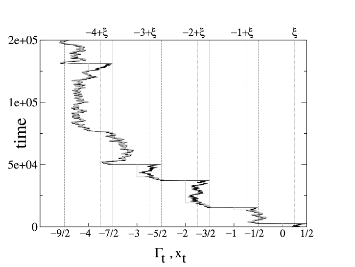
Figure 4: Typical realization of the effective translation $\Gamma_{t}$ (black line) and the corresponding particle trajectory $x_{t}$ (gray line). The dashed lines denote the ”reflection points” $x=-K+3/2$ of the trajectory $\Gamma_{t}$, while the dash-dotted lines - the special points $-K+\xi$. Vertical red lines show the special points at which the particle seizes to move.

(ii) when $\Gamma_{t}$ hits the left-hand-side boundary of the $K$-th interval and gets instantaneously transferred to the next interval, the particle makes a jump from $x_{t}=-K+\xi$ to $x_{t}=-K$. It means that although the trajectory $\Gamma_{t}$ is always continuous, the particle trajectory $x_{t}$ changes discontinuously at these points. It is clear, however, that such jumps of length $\xi$ do not contribute to the average particle velocity $\overline{\dot{x}_{t}}$. Consequently, the velocity of the effective external translation ${\cal V}=\overline{\dot{\Gamma}_{t}}$ and average particle velocity $\overline{\dot{x}_{t}}$ coincide, i.e. ${\cal V}=\overline{\dot{x}_{t}}=\overline{\dot{\Gamma}_{t}}$.

5 Zero external bias $f_{0}$.

We turn next to the computation of the velocity ${\cal V}$ focussing first on the case of zero external bias, $f_{0}=0$. Evidently, even in this simplest case the map depicted in Fig.3 is too complex to be solved exactly. However, some simple analytical arguments can be proposed to obtain very accurate estimates for the functional form of ${\cal V}$. To do this, we first note that it is only when passing from the $K$-th interval to the next, $(K+1)$-th interval, (which is displaced on a unit distance on the $\Gamma_{t}$-axis with respect to the previous one), the process $\Gamma_{t}$ gains an uncompensated (negative) displacement equal to the overlap distance of two consecutive intervals, which equals, namely, $1/2-\xi$. Consequently, ${\cal V}$ can be estimated as ${\cal V}=-(1/2-\xi)/T$, where $T$ is the mean time which the process $\Gamma_{t}$ ”spends” within a given interval. To estimate the value of $T$, let us consider more precisely dynamics of the process $\Gamma_{t}$ on a given interval.

Figure 5: Time evolution of the effective external translation $\Gamma_{t}$ on the $K$-th interval.

The time $T$ is, as a matter of fact, the mean time needed for the process $\Gamma_{t}$ to reach diffusively for the first time the left-hand-side boundary of the interval - the ”exit” point $-K+\xi$, starting from the ”entry” point $-K+1+\xi$ (see Fig.5). It is convenient now to divide the $K$-th interval into three sub-intervals: $l_{1}=l_{3}=1/2-\xi$ and $l_{2}=1/2+\xi$, Fig.5. Evidently, since $l_{1}=l_{3}\leq l_{2}$, ($\xi>0$), for typical realizations of external random force $f_{t}$, the following scenario holds: the process $\Gamma_{t}$ evolves randomly around the ”entry” point and first hits the right-hand-side boundary of the $K$-th interval passing thus through the sub-interval $l_{1}$; the mean time required for the first passage of this sub-interval is denoted as $T_{1}$. For conventional diffusion with diffusion coefficient $D$ this time is given by $T_{1}=(1/2-\xi)^{2}/2D$ [27]. Further on, after hitting the right-hand-side boundary, $\Gamma_{t}$ gets reflected to the point $\Gamma_{t}=-(2K-1)/2$ and evolves randomly around this point until it hits the left-hand-side boundary of the interval - the ”exit” point. For symmetric diffusion, the time $T_{3}$ needed for the first passage through the sub-interval $l_{3}$ is equal to $T_{1}$. Consequently, $T=T_{1}+T_{3}=(1/2-\xi)^{2}/D$ and the particle velocity follows

$${\cal V}=-\frac{2D}{1-2\xi}$$ (6)

In Fig.6 we compare our theoretical prediction in Eq.(6) and the results of the Monte Carlo simulations, which comparison shows that simple theoretical arguments presented above capture the essential physics underlying the dynamics of the random map depicted in Fig.3.

Figure 6: The absolute value of the statistical velocity $V$ versus $\xi$. The solid line gives the analytical prediction in Eq.(6) and the triangles depict Monte Carlo data. Note that we use, for notational convenience, the log-log scale.

Now, we proceed with several comments on the result in Eq.(6).
(i) First, we note that ${\cal V}$ determined by Eq.(6) increases indefinitely when $\xi\to 1/2$, although, however, ${\cal V}\equiv 0$ for $\xi\equiv 1/2$, which is a seemingly artificial discontinuity. As a matter of fact, such a behavior stems from our definition of the random process $\Gamma_{t}$; namely, by writing our Eq.(5) we tacitly assume that both the effective step $\delta\Gamma$ of the process $\Gamma_{t}$ and the characteristic jump time $\tau$ are infinitesimal variables, (while the ratio $D=(\delta\Gamma)^{2}/2\tau$ is supposed to be fixed and finite). On the other hand, for any realistic physical system $\delta\Gamma$ and $\tau$ may be very small, but nonetheless are both finite. For finite $\delta\Gamma$ and $\tau$, the process $\Gamma_{t}$ can be viewed as a hopping process on a lattice with spacing $\delta\Gamma$ and with the characteristic time separating successive jumps equal to $\tau$. The hopping probabilities are symmetric; that is, the probabilities of jumping from the site $\Gamma$ to either of its neighboring sites are equal to each other. For this model, we find for $T_{1}$ and $T_{3}$ the following forms (see, e.g., Ref.[27]):

$$T_{1}=T_{3}=\tau\Big{(}1+L\Big{)}L,$$ (7)

where $L=(1/2-\xi)/\delta\Gamma$ is the number of elementary steps $\delta\Gamma$ in the interval $(1/2-\xi)$. Equation (7) yields, in place of Eq.(6),

$${\cal V}=-\frac{2D}{2\delta\Gamma+1-2\xi}$$ (8)

Note now that for finite $\delta\Gamma$ and $\tau$ the velocity ${\cal V}$ in Eq.(8) tends to a finite value when $\xi\to 1/2$ (but still we have ${\cal V}\equiv 0$ for $\xi=1/2$). We also remark that relaxing the assumption of the overdamped motion and/or adding a noise term to Eq.(2), we will obtain a certain rounding of the behavior of ${\cal V}$ in the vicinity of $\xi=1/2$ [28]. As a matter of fact, our numerical simulations show that ${\cal V}$ becomes a smooth bell-shaped function with ${\cal V}=0$ for $\xi=1/2$ and a maximal value close to $\xi=1/2$.

(ii) Second, we notice that the velocity defined by Eqs.(6) or (8) is a monotonously increasing function of the parameter $\xi$, which defines the degree of the asymmetry of the external potential; that is, the velocity by absolute value is maximal for low asymmetry when $\xi\to 1/2$ and minimal, ${\cal V}=2D$, for the strongest asymmetry with $\xi=0$. We would like to comment now that such a behavior relies strongly on the definition of the random external force $f_{t}$ as a Gaussian, delta-correlated noise. As $f_{t}$ is the property influenced by external processes, it might be characterized, for instance, by essential correlations or be a non-local in space or in time (discontinuous) stochastic process. In both cases, the behavior of the particle’s velocity in the presence of such an external force would be different of that predicted by Eqs.(6) and (8).

Suppose, for example, that $f_{t}$ represents the so-called delta-correlated Lévy process with parameter $\mu$ (see, e.g., Ref.[27] for more discussion). We note here parenthetically that the case $\mu=2$ corresponds to the usual Gaussian case, which yields conventional diffusive motion, while the case $\mu=1$ describes the so-called Cauchy process.

Now, what basically changes when we assume that $f_{t}$ represents the Lévy process is the functional form of the first passage times $T_{1}$ and $T_{2}$. In this case the time required for the first passage of an interval of length $1/2-\xi$ reads $T_{1}=T_{3}\sim(1/2-\xi)^{\mu}$ [27] and hence, the particle velocity follows

$${\cal V}\sim-(1-2\xi)^{1-\mu}$$ (9)

Consequently, we may expect that the particle’s velocity will be a monotonously increasing function of the parameter $\xi$ only for the Lévy processes with $\mu>1$, i.e. for persistent processes (which have a finite probability for return to the origin). In the borderline case of $\mu=1$ (the Cauchy process) velocity will be independent of the asymmetry parameter. On the other hand, for transient processes with $\mu<1$, (i.e. having zero probability of return to the origin), which are not space-filling (fractal) and occupy the space in clustered or localized patches, one may expect that the particle’s velocity would be a decreasing function of the asymmetry parameter $\xi$.

6 Non-zero external bias $f_{0}$.

In this section we generalize our previous results for the generic case of non-zero averaged external force. We will consider both the situations when $f_{0}$ is negative or positive.

6.1 Positive bias

Consider first the case when the bias is oriented in the positive direction, i.e. $f_{0}\geq 0$. The salient feature of this situation is that here the asymmetry of the embedding potential prevents the particle of moving in the positive direction, i.e. in the direction of the applied field $f_{0}$. Hence, in this case if a drift motion of the particle takes place, - it would take place against the applied field! We set out to show in what follows that this is actually the case: the particle does travel with a constant velocity ${\cal V}$ in the negative direction and such an extraordinary behavior is essentially due to fluctuations in the process $\Gamma_{t}$ - some (exponentially small) number of its trajectories traveling against the external field.

Now, we suppose that the hopping process $\Gamma_{t}$ takes place on a discrete lattice with a spacing $\delta\Gamma$. Each interval in Fig.5 is thus separated into a set of $L$ elementary steps, $L=(3/2-\xi)/\delta\Gamma$. The hopping probabilities for jumps in the positive ($p$) and in the negative ($q$) directions are no longer equal and obey:

$$p/q=\exp\Big{(}\beta f_{0}\delta\gamma\Big{)},\;\;\;p+q=1,$$ (10)

where $\beta$ denotes the reciprocal temperature.

One readily notices now that in the situation under consideration the symmetry $T_{1}=T_{3}$, which existed in the case $f_{0}=0$, is broken: when passing through the sub-interval $l_{1}$ the process $\Gamma_{t}$ follows the field, while the first passage through the sub-interval $l_{3}$ takes place in the situation when the field $f_{0}$ is directed effectively against the passage direction. Supposing that $\delta\Gamma$ and $\tau$ are both finite, we have then that here [27]:

$$T_{1}=\frac{\tau\Big{(}1+\exp\Big{(}-\beta f_{0}\delta\Gamma\Big{)}\Big{)}}{\Big{(}1-\exp\Big{(}-\beta f_{0}\delta\Gamma\Big{)}\Big{)}}\Big{[}\frac{1/2-\xi}{\delta\Gamma}-$$

$$-\frac{\exp\Big{(}-\beta f_{0}\delta\Gamma\Big{)}}{\Big{(}1-\exp\Big{(}-\beta f_{0}\delta\Gamma\Big{)}\Big{)}}\Big{(}1-\exp\Big{(}-\beta f_{0}(1/2-\xi)\Big{)}\Big{)}\Big{]}$$ (11)

and

$$T_{3}=\frac{\tau\Big{(}1+\exp\Big{(}\beta f_{0}\delta\Gamma\Big{)}\Big{)}}{\Big{(}\exp\Big{(}\beta f_{0}\delta\Gamma\Big{)}-1\Big{)}}\Big{[}\frac{\exp\Big{(}\beta f_{0}\delta\Gamma\Big{)}}{\Big{(}\exp\Big{(}\beta f_{0}\delta\Gamma\Big{)}-1\Big{)}}\times$$

$$\times\Big{(}\exp\Big{(}\beta f_{0}(1/2-\xi)\Big{)}-1\Big{)}-\frac{1/2-\xi}{\delta\Gamma}\Big{]},$$ (12)

respectively.

Note that $T_{1}$ grows linearly with the sub-interval length $1/2-\xi$, while $T_{3}$ shows much stronger, exponential interval-length dependence, and hence, controls the overall time spent within a given interval.

Consequently, the particle’s velocity in this case attains the form

$${\cal V}=-\frac{(1/2-\xi)\sinh^{2}\Big{(}\beta f_{0}\delta\Gamma/2\Big{)}}{\tau\cosh\Big{(}\beta f_{0}\delta\Gamma/2\Big{)}\Big{[}\cosh\Big{(}\beta f_{0}(1-2\xi+\delta\Gamma)/2\Big{)}-\cosh\Big{(}\beta f_{0}\delta\Gamma/2\Big{)}\Big{]}}$$ (13)

We note again that the remarkable feature of this results is that it predicts a drift motion of the particle against the applied external field $f_{0}$.

In the diffusion limit, i.e. when $\delta\Gamma$ and $\tau$ are set equal to zero but the ratio $(\delta\Gamma)^{2}/\tau$ is kept fixed, we find from Eq.(13) the following result:

$${\cal V}=-\frac{(1-2\xi)D\beta^{2}f_{0}^{2}}{8\sinh^{2}\Big{(}\beta f_{0}(1-2\xi)/4\Big{)}},$$ (14)

which reduces to the result in Eq.(6) when $f_{0}\to 0$.

6.2 Negative bias

We turn next to the case of negative bias, $f_{0}<0$. At the first glance, this case should not give us any surprise - one anticipates that the particle here will always be passively carried by the field. It appears, however, that such a behavior may take place only for sufficiently low asymmetries of the saw-tooth potential. For high asymmetries $\xi$, it may appear that it will be more efficient for the particle to travel through the shorter interval ($l_{1}$, Fig.5) against the field, than to be carried passively through the longer interval $l_{2}$. It means that exponentially small number of trajectories travelling against the field will still matter, as in the case of positive bias. Consequently, this will give rise to a cusp in the overall dependence ${\cal V}(\xi)$.

We turn now to the analysis of the characteristic passage times involved in this case. We start first with the passage through the sub-interval $l_{3}$, in which a particle appearing at some time at the point $-(2K-1)/2$ should travel to the ”exit” point $-K+\xi$. The passage through this sub-interval is favored by the field $f_{0}$ and the first passage time is given by

$$T_{3}=\frac{\tau\Big{(}1+\exp\Big{(}\beta f_{0}\delta\Gamma\Big{)}\Big{)}}{\Big{(}1-\exp\Big{(}\beta f_{0}\delta\Gamma\Big{)}\Big{)}}\Big{[}\frac{1/2-\xi}{\delta\Gamma}-$$

$$-\frac{\exp\Big{(}\beta f_{0}\delta\Gamma\Big{)}}{\Big{(}1-\exp\Big{(}\beta f_{0}\delta\Gamma\Big{)}\Big{)}}\Big{(}1-\exp\Big{(}\beta f_{0}(1/2-\xi)\Big{)}\Big{)}\Big{]}$$ (15)

Now, the question what is the mean time typically needed to reach this point $-(2K-1)/2$ starting from the ”entry” point $-K+1+\xi$ is a bit more delicate: it can be reach either by the field-enhanced diffusion through the larger sub-interval $l_{2}$ or by diffusion against the field $f_{0}$ through the smaller sub-interval $l_{1}$ to the right-hand-side boundary of the interval (the ”reflection” point) followed by an instantaneous transfer to the point $-(2K-1)/2$ (see, Fig.3). Two respective mean first passage times are given here by

$$T_{2}=\frac{\tau\Big{(}1+\exp\Big{(}\beta f_{0}\delta\Gamma\Big{)}\Big{)}}{\Big{(}1-\exp\Big{(}\beta f_{0}\delta\Gamma\Big{)}\Big{)}}\Big{[}\frac{1/2+\xi}{\delta\Gamma}-$$

$$-\frac{\exp\Big{(}\beta f_{0}\delta\Gamma\Big{)}}{\Big{(}1-\exp\Big{(}\beta f_{0}\delta\Gamma\Big{)}\Big{)}}\Big{(}1-\exp\Big{(}\beta f_{0}(1/2+\xi)\Big{)}\Big{)}\Big{]}$$ (16)

and

$$T_{1}=\frac{\tau\Big{(}1+\exp\Big{(}\beta f_{0}\delta\Gamma\Big{)}\Big{)}}{\Big{(}1-\exp\Big{(}\beta f_{0}\delta\Gamma\Big{)}\Big{)}}\Big{[}\frac{\Big{(}\exp\Big{(}\beta f_{0}(1/2-\xi)\Big{)}\Big{)}-1}{\Big{(}1-\exp\Big{(}-\beta f_{0}\delta\Gamma\Big{)}\Big{)}}-\frac{1/2-\xi}{\delta\Gamma}\Big{]}$$ (17)

The particle velocity ${\cal V}$ thus can be estimated as:

$${\cal V}=-\frac{(1/2-\xi)}{T_{3}+min(T_{1},T_{2})}$$ (18)

If $T_{1}<T_{2}$, we would evidently recover our previous result in Eq.(13) up to the reversal of the sign, $f_{0}\to-f_{0}$. In the opposite case, $T_{1}>T_{2}$, one finds

$${\cal V}=-\frac{(1/2-\xi)\delta\Gamma}{\tau\coth\Big{(}-\beta f_{0}\delta\Gamma/2\Big{)}}\Big{[}1-\frac{2\delta\Gamma\exp\Big{(}\beta f_{0}\delta\Gamma\Big{)}}{1-\exp\Big{(}\beta f_{0}\delta\Gamma\Big{)}}\times$$

$$\times\Big{(}1-\exp\Big{(}\beta f_{0}\delta\Gamma/2\Big{)}\cosh\Big{(}(\beta f_{0}\delta\Gamma\xi\Big{)}\Big{)}\Big{]}^{-1}$$ (19)

Now, on comparing $T_{1}$ and $T_{2}$ we find that these two mean first passage times are equal to each other when the following equality holds:

$$\xi=\xi_{crit}=\frac{\ln\Big{(}\cosh\Big{(}\beta f_{0}\delta\Gamma/2\Big{)}\Big{)}}{\Big{(}-\beta f_{0}\delta\Gamma\Big{)}}$$ (20)

Hence, for fixed $\beta f_{0}\delta\Gamma$, $T_{1}<T_{2}$ and the particle velocity is described by Eq.(13) with $f_{0}$ changed for $-f_{0}$ when

$$\xi>\xi_{crit}$$ (21)

Otherwise, $T_{2}<T_{1}$ and the particle velocity obeys Eq.(6.2). This means that the overall dependence of the particle velocity on the asymmetry parameter will have a cusp at $\xi=\xi_{crit}$. Note also that $\xi_{crit}$ is a monotonously increasing function of the parameter $(-\beta f_{0}\delta\Gamma)$, which equals zero when $\beta f_{0}\delta\Gamma=0$ and rapidly approaches $1/2$ when $(-\beta f_{0}\delta\Gamma)\to\infty$. Hence, $\xi$ should be sufficiently close to its maximal value $1/2$ in order that the behavior predicted by Eq.(13) takes place in the case of a negative bias.

7 Conclusion

In conclusion, we have studied dynamics of a classical particle in a 1D potential, composed of two periodic, asymmetric saw-tooth components, one of which is driven by an external random force. Concentrating on the overdamped limit, we presented analytical estimates for the particle’s velocity. We have shown that in such a system the particle will perform a $unidirectional$ saltatory drift regardless of the fact whether the average force is zero, or directed against the particle motion. In case when the average force is negative and its direction coincides with the direction of the particle motion, we predicted a cusp-like dependence of the particle velocity on the asymmetry parameter of the saw-tooth potential. We have demonstrated that the physical mechanism underlying such a behavior resembles the work of the so-called escapement device, used by watchmakers to convert the raw power of the driving force into uniform impulses. Here, indeed, upon reaching certain levels, random forces lock the particle’s motion creating points of irreversibility, so that the particle gets uncompensated displacements. Repeated (randomly) in each cycle, this process ultimately results in a saltatory drift with random pausing times. Our analytical results for systems in which the random force averages out to zero are in a very good agreement with Monte Carlo data.

8 Acknowledgments

The authors gratefully acknowledge helpful discussions with M.Porto. GO thanks the AvH Foundation for the financial support via the Bessel Research Award.

References

References

- [1] Maxwell J C 1872 Theory of Heat (Longmans, Green and Co, London)
- [2] von Smoluchowski M 1912 Phys. Z 13 p 1069
- [3] Feynman R P, Leighton R B and Sands M 1963 The Feynman Lectures on Physics (Addison-Wesley, Reading)
- [4] Curie M P 1894 J. Phys. (Paris) III 3 p 393
- [5] Ajdari A and Prost J 1993 C.R. Acad. Sci. Paris II 315 p 1635
- [6] Magnasco M O 1993 Phys. Rev. Lett. 71 p 1477
- [7] Astumian R D and Bier M 1994 Phys. Rev. Lett. 72 p 1766
- [8] Duke T, Holy T E and Leibler S 1995 Phys. Rev. Lett. 74 p 330
- [9] Astumian R D 1997 Science 276 p 917
- [10] Dialynas T E, Lindenberg K and Tsironis G P 1997 Phys. Rev. E 56 p 3976
- [11] Sokolov I M 1998 Europhys. Lett. 44 p 278; Phys. Rev. E 60 p 4946
- [12] Fisher M E and A.B.Kolomeisky A B 1999 Proc. Natl. Acad. Sci. USA 96 p 6597
- [13] Lipowski R 2000 Phys. Rev. Lett. 85 p 4401
- [14] Porto M, Urbakh M and Klafter J 2000 Phys. Rev. Lett. 85 p 491
- [15] Popescu M N, Arizmendi C M, Salas-Brito A L and Family F 2000 Phys. Rev. Lett. 85 p 3321
- [16] Lipowski R, Klumpp S and Nieuwenhuizen T M 2001 Phys. Rev. Lett. 87 p 108101
- [17] Rousselet J, Salome L, Ajdari A and Prost J 1994 Nature 370 p 446
- [18] Faucheux L P, Bourdieu L S, Kaplan P D and Libchaber A J 1995 Phys. Rev. Lett. 74 p 1504
- [19] Gorre L, Ioannidis E and Silberzan P 1996 Europhys. Lett. 33 p 267
- [20] Kettner C, Reimann P, Hänggi P and Müller F 2000 Phys. Rev. E 61 p 312
- [21] Jülicher F, Ajdari A and Prost J 1997 Rev. Mod. Phys. 69 p 126
- [22] Reimann P and Hänggi P 2002 Appl. Phys. A 75 p 169
- [23] Reimann P 2002 Phys. Repts. 361 p 57
- [24] Astumian R D and Hänggi P 2002 Physics Today (November 22) p 33
- [25] http://www.horologia.co.uk/escapements.html
- [26] Oshanin G, Klafter J and Urbakh M 2004 Europhys. Lett. 68 p 26
- [27] Lindenberg K and West B J 1986 J. Stat. Phys. 42 p 201
- [28] Oshanin G, Klafter J and Urbakh M, in preparation