Simulation of thin hyperelastic shells with the Material Point Method

Abstract

A non-linear shell theory that includes transverse shear strains and its implementation in the material point method framework are discussed. The applicability of the shell implementation to model large deformations of thin shells is explored. Results suggest that an implicit time stepping scheme may be required for improved modeling of thin shells by the material point method.

1 Shell Formulation

The continuum-based approach to shell theory has been chosen because of the relative ease of implementation of constitutive models in this approach compared to exact geometrical descriptions of the shell. In order to include transverse shear strains in the shell, a modified Reissner-Mindlin assumption is used. The major assumptions of the shell formulation are [1, 2]

1. The normal to the mid-surface of the shell remains straight but not necessarily normal. The direction of the initial normal is called the “fiber” direction and it is the evolution of the fiber that is tracked.

2. The stress normal to the mid-surface vanishes (plane stress)

3. The momentum due to the extension of the fiber and the momentum balance in the direction of the fiber are neglected.

4. The curvature of the shell at a material point is neglected.

The shell formulation is based on a plate formulation by Lewis et al.  [2]. A discussion of the formulation follows.

The velocity field in the shell is given by

$$\mathbf{w}(\alpha,\beta)=\mathbf{u}(\alpha,\beta)+z~{}\boldsymbol{\omega}(\alpha,\beta)\times\mathbf{n}(\alpha,\beta)+\dot{z}~{}\mathbf{n}(\alpha,\beta)$$ (1)

where $\mathbf{w}$ is the velocity of a point in the shell, $\mathbf{u}$ is the velocity of the center of mass of the shell, $\mathbf{n}$ is the normal or director vector, $\boldsymbol{\omega}$ is the angular velocity of the director, $(\alpha,\beta)$ are orthogonal co-ordinates on the mid-surface of the shell, $z$ is the perpendicular distance from the mid-surface of the shell, and $\dot{z}$ is the rate of change of the length of the shell director.

Since momentum balance is not enforced for the motion in the direction of the director $\mathbf{n}$, the terms involving $\dot{z}$ are dropped in constructing the equations of motion. These terms are also omitted in the deformation gradient calculation. However, the thickness change in the shell is not neglected in the computation of internal forces and moments. Equation (1) can therefore be written as

$$\mathbf{w}(\alpha,\beta)=\mathbf{u}(\alpha,\beta)+z~{}\mathbf{r}(\alpha,\beta)$$ (2)

where $\mathbf{r}$, the rotation rate of $\mathbf{n}$, is a vector that is perpendicular to $\mathbf{n}$.

The velocity gradient tensor for $\mathbf{w}$ is used to compute the stresses in the shell. If the curvature of the shell is neglected, i.e., the shell is piecewise plane, the velocity gradient tensor for $\mathbf{w}$ can be written as

$$\boldsymbol{\nabla}\mathbf{w}=\left[\boldsymbol{\nabla}^{(s)}\mathbf{u}+z~{}\boldsymbol{\nabla}^{(s)}\mathbf{r}\right]+\mathbf{r}\otimes\mathbf{n}$$ (3)

where $\mathbf{r}\otimes\mathbf{n}$ represents the dyadic product, and $\mathbf{\nabla}^{(s)}$ is the in-surface gradient operator, defined as,

$$\boldsymbol{\nabla}^{(s)}=\left[\boldsymbol{\nabla}(~{}~{})\right]\bullet\mathbf{I}^{(s)}~{}.$$ (4)

The $\bullet$ represents a tensor inner product and $\mathbf{I}^{(s)}$ is the in-surface identity tensor (or the projection operator), defined as,

$$\mathbf{I}^{(s)}=\mathbf{I}-\mathbf{n}\otimes\mathbf{n}.$$ (5)

It should be noted that, for accuracy, the vector $\mathbf{n}$ should not deviate significantly from the actual normal to the surface (i.e., the transverse shear strains should be small).

The determination of the shell velocity tensor $\boldsymbol{\nabla}\mathbf{w}$ requires the determination of the center of mass velocity $\mathbf{u}$ of the shell. This quantity is determined using the balance of linear momentum in the shell. The local three-dimensional equation of motion for the shell is, in the absence of body forces,

$$\boldsymbol{\nabla}\bullet\boldsymbol{\sigma}=\rho~{}\mathbf{a}$$ (6)

where $\mathbf{sigma}$ is the stress tensor, $\rho$ is the density of the shell material, and $\mathbf{a}$ is the acceleration of the shell. The two-dimensional form of the linear momentum balance equation  (6) with respect to the surface of the shell is given by

$$\boldsymbol{\nabla}^{(s)}\bullet\left<\boldsymbol{\sigma}\right>=\rho~{}\mathbf{a}~{}.$$ (7)

The acceleration of the material points in the shell are now due to the in-surface divergence of the average stress $\left<\boldsymbol{\sigma}\right>$ in the shell, given by

$$\left<\boldsymbol{\sigma}\right>\colon=\frac{1}{h}\int^{h^{+}}_{-h^{-}}\boldsymbol{\sigma}(z)~{}dz$$ (8)

where $h^{+}$ is the “thickness” of the shell (along the director) from the center of mass to the “top” of the shell, $h^{-}$ is the thickness from the center of mass to the “bottom” of the shell, and $h=h^{+}+h^{-}$. The point of departure from the formulation of Lewis et al. [2] is that instead of separate linear momentum balance laws for shell and non-shell materials, a single global momentum balance is used and the “plane stress” condition $\mathbf{\sigma}_{zz}=0$ is enforced in the shell stress update, where the subscript $zz$ represents the direction of the shell director.

The shell director $\mathbf{n}$ and its rotation rate $\mathbf{r}$ also need to be known before the shell velocity gradient tensor $\boldsymbol{\nabla}\mathbf{w}$ can be determined. These quantities are determined using an equation for the conservation of angular momentum [3], given by

$$\boldsymbol{\nabla}^{(s)}\bullet\mathbf{M}-\mathbf{n}\bullet\left<\boldsymbol{\sigma}\right>\bullet\mathbf{I}^{(s)}=\frac{1}{12}~{}\rho~{}h^{2}~{}\dot{\mathbf{r}}$$ (9)

where $\dot{\mathbf{r}}$ is the rotational acceleration of $\mathbf{n}$, $\rho$ is the density of the shell material, and $\mathbf{M}$ is the average moment, defined as

$$\mathbf{M}\colon=\mathbf{I}^{(s)}\bullet\left[\frac{1}{h}\int^{h^{+}}_{-h^{-}}\boldsymbol{\sigma}(z)~{}z~{}dz\right]\bullet\mathbf{I}^{(s)}~{}.$$ (10)

The center-of-mass velocity $\mathbf{u}$, the director $\mathbf{n}$ and its rate of rotation $\mathbf{r}$ provide a means to obtain the velocity of material points on the shell. The shell is divided into a number of layers with discrete values of $z$ and the layer-wise gradient of the shell velocity is used to compute the stress and deformation in each layer of the shell.

2 Shell Implementation for the Material Point Method

The shell description given in the previous section has been implemented such that the standard steps of the material point method [4] remain the same for all materials. Some additional steps are performed for shell materials. These steps are encapsulated within the shell constitutive model.

The steps involved for each time increment $\Delta t$ are discussed below. The superscript $n$ represents the value of the state variables at time $n~{}\Delta t$ while the superscript $n+1$ represents the value at time $(n+1)~{}\Delta t$. Note that $\Delta t$ need not necessarily be constant. In the following, the subscript $p$ is used to index material point variables while the subscript $v$ is used to index grid vertex variables. The notation $\sum_{p}$ denotes summation over material points and $\sum_{v}$ denotes summation over grid vertices. Zeroth order interpolation functions associated with each material point are denoted by $S^{(0)}_{p,v}$ while first order interpolation functions are denoted by $S^{(1)}_{p,v}$.

1. Interpolate state data from material points to the grid.
   The state variables are interpolated from the material points to the grid vertices using the contiguous generalized interpolation material point (GIMP) method [5]. In the GIMP method material points are defined by particle characteristic functions $\chi_{p}(\mathbf{x})$ which are required to be a partition of unity,

   $$\sum_{p}\chi_{p}(\mathbf{x})=1~{}~{}\forall~{}~{}\mathbf{x}\in\Omega$$ (11)

   where $\mathbf{x}$ is the position of a point in the body $\Omega$. A continuous representation of the property $f(\mathbf{x})$ is given by

   $$f(\mathbf{x})=\sum_{p}f_{p}~{}\chi_{p}(\mathbf{x})~{}$$ (12)

   where $f_{p}$ is the value at a material point. Similarly, a continuous representation of the grid data is given by

   $$g(\mathbf{x})=\sum_{v}g_{v}~{}S_{v}(\mathbf{x})~{}$$ (13)

   where

   $$\sum_{v}S_{v}(\mathbf{x})=1~{}~{}\forall~{}~{}\mathbf{x}\in\Omega~{}.$$ (14)

   To interpolate particle data to the grid, the interpolation (or weighting functions) $S^{(1)}_{p,v}$ are used, which are defined as

   $$S^{(1)}_{p,v}=\frac{1}{V_{p}}\int_{\Omega_{p}\cap\Omega}\chi_{p}(\mathbf{x})~{}S_{v}(\mathbf{x})~{}d{\mathbf{x}}~{}$$ (15)

   where $V_{p}$ is the volume associated with a material point, $\Omega_{p}$ is the region of non-zero support for the material point, and

   $$\sum_{v}S^{(1)}_{p,v}=1~{}~{}\forall~{}~{}\mathbf{x_{p}}\in\Omega_{p}~{}.$$ (16)

   The state variables that are interpolated to the grid in this step are the mass ($m$), momentum ($m\mathbf{u}$), volume ($V$), external forces ($\mathbf{f}^{\text{ext}}$), temperature ($T$), and specific volume ($v$) using relations of the form

   $$m_{v}=\sum_{p}m_{p}~{}S^{(1)}_{p,v}~{}.$$ (17)

   In our computations, bilinear hat functions $S_{v}$ were used that lead to interpolation functions $S^{(1)}_{p,v}$ with non-zero support in adjacent grid cells and in the next nearest neighbor grid cells. Details of these functions can be found in reference [5].

   For shell materials, an additional step is required to inhabit the grid vertices with the interpolated normal rotation rate from the particles. However, instead of interpolating the angular momentum, the quantity $\mathbf{p}_{p}=m_{p}\mathbf{r}_{p}$ is interpolated to the grid using the relation

   $$\mathbf{p}_{v}=\sum_{p}\mathbf{p}_{p}~{}S^{(1)}_{p,v}~{}.$$ (18)

   At the grid, the rotation rate is recovered using

   $$\mathbf{r}_{v}=\mathbf{p}_{v}/m_{v}$$ (19)

   This approximation is required because the moment of inertia contains $h^{2}$ terms which can be very small for thin shells. Floating point errors are magnified when $m_{p}$ is multiplied by $h^{2}$. In addition, it is not desirable to interpolate the plate thickness to the grid.

2. Compute heat and momentum exchange due to contact.
   In this step, any heat and momentum exchange between bodies inside the computational domain is performed through the grid. Details of contact algorithms used my the material point method can be found in references [4, 6, 7].

3. Compute the stress tensor.
   The stress tensor computation follows the procedure for hyperelastic materials cited in reference [8]. However, some extra steps are required for shell materials. The stress update is performed using a forward Euler explicit time stepping procedure. The velocity gradient $\boldsymbol{\nabla}\mathbf{w}$ at a material point is required for the stress update. This quantity is determined using equation (3). The velocity gradient of the center of mass of the shell ($\boldsymbol{\nabla}\mathbf{u}$) is computed from the grid velocities using gradient weighting functions of the form

   $$\boldsymbol{\nabla}S^{(1)}_{p,v}=\frac{1}{V_{p}}\int_{\Omega_{p}\cap\Omega}\chi_{p}(\mathbf{x})~{}\boldsymbol{\nabla}S_{v}(\mathbf{x})~{}d{\mathbf{x}}$$ (20)

   so that

   $$\boldsymbol{\nabla}\mathbf{u}_{p}=\sum_{v}\mathbf{u}_{v}~{}\boldsymbol{\nabla}S^{(1)}_{p,v}~{}.$$ (21)

   The gradient of the rotation rate ($\boldsymbol{\nabla}\mathbf{r}$) is also interpolated to the particles using the same procedure, i.e.,

   $$\boldsymbol{\nabla}\mathbf{r}_{p}=\sum_{v}\mathbf{r}_{v}~{}\boldsymbol{\nabla}S^{(1)}_{p,v}~{}.$$ (22)

   The next step is to calculate the in-surface gradients $\boldsymbol{\nabla}^{(s)}\mathbf{u}_{p}$ and $\boldsymbol{\nabla}^{(s)}\mathbf{r}_{p}$. These are calculated as

   $$\boldsymbol{\nabla}^{(s)}\mathbf{u}_{p} =\boldsymbol{\nabla}\mathbf{u}_{p}\bullet\left(\mathbf{I}-\mathbf{n}^{n}_{p}\otimes\mathbf{n}^{n}_{p}\right)$$ (23)

   $$\boldsymbol{\nabla}^{(s)}\mathbf{r}_{p} =\boldsymbol{\nabla}\mathbf{r}_{p}\bullet\left(\mathbf{I}-\mathbf{n}^{n}_{p}\otimes\mathbf{n}^{n}_{p}\right)$$ (24)

   The superscript $n$ represents the values at the end of the $n$-th time step. The shell is now divided into a number of layers with different values of $z$ (these can be considered to be equivalent to Gauss points to be used in the integration over $z$). The number of layers depends on the requirements of the problem. Three layers are used to obtain the results that follow. The velocity gradient $\boldsymbol{\nabla}\mathbf{w}_{p}$ is calculated for each of the layers using equation (3). For a shell with three layers (top, center and bottom), the velocity gradients are given by

   $$\boldsymbol{\nabla}\mathbf{w}_{p}^{\text{top}} =\left[\boldsymbol{\nabla}^{(s)}\mathbf{u}_{p}+h^{+}~{}\boldsymbol{\nabla}^{(s)}\mathbf{r}_{p}\right]+\mathbf{r}_{p}^{n}\otimes\mathbf{n}_{p}^{n}$$ (25)

   $$\boldsymbol{\nabla}\mathbf{w}_{p}^{\text{cen}} =\boldsymbol{\nabla}^{(s)}\mathbf{u}_{p}+\mathbf{r}_{p}^{n}\otimes\mathbf{n}_{p}^{n}$$ (26)

   $$\boldsymbol{\nabla}\mathbf{w}_{p}^{\text{bot}} =\left[\boldsymbol{\nabla}^{(s)}\mathbf{u}_{p}-h^{-}~{}\boldsymbol{\nabla}^{(s)}\mathbf{r}_{p}\right]+\mathbf{r}_{p}^{n}\otimes\mathbf{n}_{p}^{n}$$ (27)

   The increment of deformation gradient ($\Delta\mathbf{F}$) in each layer is computed using

   $$\Delta\mathbf{F}_{p}=\Delta t~{}\boldsymbol{\nabla}\mathbf{w}_{p}+\mathbf{I}$$ (28)

   The total deformation gradient ($\mathbf{F}$) in each layer is updated using

   $$\boldsymbol{\tilde{\mathbf{F}}}_{p}^{n+1}=\Delta\mathbf{F}_{p}\bullet\mathbf{F}_{p}^{n}$$ (29)

   where $\boldsymbol{\tilde{\mathbf{F}}}_{p}^{n+1}$ is the intermediate updated deformation gradient prior to application of the “plane stress” condition.

   The stress in the shell is computed using a stored energy function ($W$) of the form

   $$W=\frac{1}{2}K\left[\frac{1}{2}(J^{2}-1)-\ln J\right]+\frac{1}{2}G\left[\text{tr}(\boldsymbol{\bar{\mathbf{b}}})-3\right]$$ (30)

   where $K$ is the bulk modulus, $G$ is the shear modulus, $J$ is the Jacobian ($J=\text{det}~{}\mathbf{F}$), and $\boldsymbol{\bar{\mathbf{b}}}$ is the volume preserving part of the left Cauchy-Green strain tensor, defined as

   $$\boldsymbol{\bar{\mathbf{b}}}\colon=J^{-\frac{2}{3}}\mathbf{F}\bullet\mathbf{F}^{T}$$ (31)

   The Cauchy stress then has the form

   $$\boldsymbol{\sigma}=\frac{1}{2}K\left(J-\frac{1}{J}\right)\mathbf{I}+\frac{G}{J}\left[\boldsymbol{\bar{\mathbf{b}}}-\frac{1}{3}\text{tr}(\boldsymbol{\bar{\mathbf{b}}})\right]~{}.$$ (32)

   The “plane stress” condition in the thickness direction of the shell is applied at this stage using an iterative Newton method. To apply this condition, the deformation gradient tensor has to be rotated such that its $(33)$ component is aligned with the $(zz)$ direction of the shell. The rotation tensor is the one required to rotate the vector $\mathbf{e}_{3}\equiv(0,0,1)$ to the direction $\mathbf{n}_{p}^{n}$ about the vector $\mathbf{e}_{3}\times\mathbf{n}_{p}^{n}$. If $\theta$ is the angle of rotation and $\mathbf{a}$ is the unit vector along axis of rotation, the rotation tensor is given by (using the derivative of the Euler-Rodrigues formula)

   $$\mathbf{R}=\cos\theta\left(\mathbf{I}-\mathbf{a}\otimes\mathbf{a}\right)+\mathbf{a}\otimes\mathbf{a}-\sin\theta~{}\mathbf{A}$$ (33)

   where

   $$\mathbf{A}=\begin{bmatrix}0&-a_{3}&a_{2}\\ a_{3}&0&-a_{1}\\ -a_{2}&a_{1}&0\end{bmatrix}~{}.$$ (34)

   The rotated deformation gradient in each layer is given by

   $$\mathbf{F}_{p}^{\text{rot}}=\mathbf{R}\bullet\boldsymbol{\tilde{\mathbf{F}}}_{p}^{n+1}\bullet\mathbf{R}^{T}~{}.$$ (35)

   The updated stress ($\boldsymbol{\sigma}_{p}^{\text{rot}}$) is calculated in this rotated coordinate system using equation (32). Thus,

   $$\boldsymbol{\sigma}_{p}^{\text{rot}}=\frac{1}{2}K\left(J_{p}^{\text{rot}}-\frac{1}{J_{p}^{\text{rot}}}\right)\mathbf{I}+\frac{G}{J_{p}^{\text{rot}}}\left[\boldsymbol{\bar{\mathbf{b}}}_{p}^{\text{rot}}-\frac{1}{3}\text{tr}(\boldsymbol{\bar{\mathbf{b}}}_{p}^{\text{rot}})\right]~{}.$$ (36)

   An iterative Newton method is used to determine the deformation gradient component $F_{33}$ for which the stress component $\sigma_{33}$ is zero. The “plane stress” deformation gradient is denoted $\boldsymbol{\overset{\circ}{\mathbf{F}}}$ and the stress is denoted $\boldsymbol{\overset{\circ}{\sigma}}$.

   At this stage, the updated thickness of the shell at a material point is calculated from the relations

   $$h^{+}_{n+1} =h^{+}_{0}\int^{1}_{0}\overset{\circ}{F}_{zz}(+z)~{}dz$$ (37)

   $$h^{-}_{n+1} =h^{-}_{0}\int^{1}_{0}\overset{\circ}{F}_{zz}(-z)~{}dz$$ (38)

   where $h^{+}_{0}$ and $h^{-}_{0}$ are the initial values, and $h^{+}_{n+1}$ and $h^{-}_{n+1}$ are the updated values, of $h^{+}$ and $h^{-}$, respectively.

   In the next step, the deformation gradient and stress values for all the layers at each material point are rotated back to the original coordinate system. The updated Cauchy stress and deformation gradient are

   $$\mathbf{F}_{p}^{n+1} =\mathbf{R}^{T}\bullet\boldsymbol{\overset{\circ}{\mathbf{F}}}\bullet\mathbf{R}$$ (39)

   $$\boldsymbol{\sigma}_{p}^{n+1} =\mathbf{R}^{T}\bullet\boldsymbol{\overset{\circ}{\sigma}}\bullet\mathbf{R}~{}.$$ (40)

   The deformed volume of the shell is approximated using the Jacobian of the deformation gradient at the center of mass of the shell

   $$V_{p}^{n+1}=V_{p}^{0}~{}J_{p}^{n+1}~{}.$$ (41)

4. Compute the internal force and moment.
   The internal force for general materials is computed at the grid using the relation

   $$\mathbf{f}_{v}^{\text{int}}=\sum_{p}\left[\boldsymbol{\sigma}_{p}^{n+1}\bullet\boldsymbol{\nabla}S^{(1)}_{p,v}\right]~{}V_{p}^{n+1}$$ (42)

   For shell materials, this relation takes the form

   $$\mathbf{f}_{v}^{\text{int}}=\sum_{p}\left[\left<\boldsymbol{\sigma}_{p}^{n+1}\right>\bullet\boldsymbol{\nabla}S^{(1)}_{p,v}\right]~{}V_{p}^{n+1}$$ (43)

   In addition to internal forces, the formulation for shell materials requires the computation of internal moments in order to solve for the rotational acceleration in the rotational inertia equation  (9). To obtain the discretized form of equation  (9), the equation is integrated over the volume of the shell leading to [2]

   $$-\sum_{p}\left[\left(\mathbf{M}_{p}\bullet\boldsymbol{\nabla}S^{(1)}_{p,v}\bullet\mathbf{I}^{(s)}\right)+\left(\mathbf{n}_{p}\bullet\left<\boldsymbol{\sigma}_{p}\right>\bullet\mathbf{I}^{(s)}\right)~{}S^{(0)}_{p,v}\right]~{}V_{p}=\left(\frac{1}{12}\sum_{p}S^{(0)}_{p,v}~{}m_{p}~{}h^{2}_{p}\right)\dot{\mathbf{r}}_{v}~{}.$$ (44)

   The average stress over the thickness of the shell is calculated using equation (8) and the average moment is calculated using equation (10). The trapezoidal rule is used in both cases. Thus,

   $$\left<\boldsymbol{\sigma}_{p}^{n+1}\right> =\frac{1}{h_{n+1}}\int^{h^{+}_{n+1}}_{-h^{-}_{n+1}}\boldsymbol{\sigma}^{n+1}_{p}(z)~{}dz$$ (45)

   $$\mathbf{M}_{p}^{n+1} =\mathbf{I}^{(s)}\bullet\left[\frac{1}{h_{n+1}}\int^{h^{+}_{n+1}}_{-h^{-}_{n+1}}\boldsymbol{\sigma}_{p}^{n+1}(z)~{}z~{}dz\right]\bullet\mathbf{I}^{(s)}$$ (46)

   where

   $$\mathbf{I}^{(s)}=\mathbf{I}-\mathbf{n}_{p}^{n}\otimes\mathbf{n}_{p}^{n}$$ (47)

   These are required in the balance of rotational inertia that is used to compute the updated rotation rate and the updated director vector. The internal moment for the shell material points can therefore the calculated using

   $$\mathbf{m}_{v}^{\text{int}}=\sum_{p}\left[\left(\mathbf{M}_{p}^{n+1}\bullet\boldsymbol{\nabla}S^{(1)}_{p,v}\bullet\mathbf{I}^{(s)}\right)+\left(\mathbf{n}_{p}^{n}\bullet\left<\boldsymbol{\sigma}_{p}^{n+1}\right>\bullet\mathbf{I}^{(s)}\right)~{}S^{(0)}_{p,v}\right]~{}V_{p}^{n+1}$$ (48)

   In practice, only the first term of equation (48) is interpolated to the grid and back to the particles. The equation of motion for rotational inertia is solved on the particles.

5. Solve the equations of motion.
   The equations of motion for linear momentum are solved on the grid so that the acceleration at the grid vertices can be determined. The relation that is used is

   $$\mathbf{\dot{u}}_{v}=\frac{1}{m_{v}}\left(\mathbf{f}_{v}^{\text{ext}}-\mathbf{f}_{v}^{\text{int}}\right)$$ (49)

   where $\mathbf{f}^{\text{ext}}$ are external forces.

   The angular momentum equations are solved on the particles after interpolating the term

   $$\mathbf{\tilde{m}}_{v}=\sum_{p}\left(\mathbf{M}_{p}^{n+1}\bullet\boldsymbol{\nabla}S^{(1)}_{p,v}\bullet\mathbf{I}^{(s)}\right)$$ (50)

   back to the material points to get $\mathbf{\tilde{m}}_{p}$. The rotational acceleration is calculated using

   $$\dot{\mathbf{r}}_{p}=\left(\frac{12~{}V_{p}}{m_{p}~{}h^{2}_{p}}\right)\left[\mathbf{m}_{p}^{\text{ext}}-\mathbf{\tilde{m}}_{p}-\mathbf{n}_{p}\bullet\left<\boldsymbol{\sigma}_{p}\right>\bullet\mathbf{I}^{(s)}\right]$$ (51)

6. Integrate the acceleration.
   The linear acceleration in integrated using a forward Euler rule on the grid, giving the updated velocity on the grid as

   $$\mathbf{u}_{v}^{n+1}=\mathbf{u}_{v}^{n}+\Delta t~{}\mathbf{\dot{u}}_{v}$$ (52)

   For the rotational acceleration, the same procedure is followed at each material point to obtain an intermediate increment

   $$\Delta\mathbf{\tilde{r}}_{p}=\Delta t~{}\mathbf{\dot{r}}_{p}$$ (53)

   The factor $m_{p}~{}h^{2}_{p}$ in the denominator of the right hand side of equation (51) makes the differential equation stiff. An accurate solution of the equation requires an implicit integration or extremely small time steps. Instead, an implicit correction is made to $\Delta\mathbf{\tilde{r}}_{p}$ by solving the equation [9]

   $$\left[\mathbf{I}+\beta\left(\mathbf{I}-\mathbf{n}_{p}^{n}\otimes\mathbf{n}_{p}^{n}\right)\right]\Delta\overset{\circ}{\mathbf{r}}_{p}=\Delta\mathbf{\tilde{r}}_{p}$$ (54)

   where $\Delta\overset{\circ}{\mathbf{r}}_{p}$ is the corrected value of $\Delta\mathbf{\tilde{r}}_{p}$ and

   $$\beta=\frac{6~{}E}{V_{p}~{}m_{p}}\left(\frac{\Delta t}{h}\right)^{2}$$ (55)

   which uses the Young’s modulus $E$ of the shell material. The intermediate rotation rate is updated using the corrected increment. Thus,

   $$\mathbf{\overset{\star}{r}}_{p}^{n+1}=\mathbf{r}_{p}^{n}+\Delta\overset{\circ}{\mathbf{r}}_{p}~{}.$$ (56)

7. Update the shell director and rotate the rotation rate At this stage, the shell director at each material point is updated. The incremental rotation tensor $\Delta\mathbf{R}$ is calculated using equation (33) with rotation angle $\theta=|r|\Delta t$ and axis of rotation

   $$\mathbf{a}=\frac{\mathbf{n}_{p}^{n}\times\mathbf{\overset{\star}{r}}_{p}^{n+1}}{|\mathbf{n}_{p}^{n}\times\mathbf{\overset{\star}{r}}_{p}^{n+1}|}~{}.$$ (57)

   The updated director is

   $$\mathbf{n}_{p}^{n+1}=\Delta\mathbf{R}\bullet\mathbf{n}_{p}^{n}~{}.$$ (58)

   In addition, the rate of rotation has to be rotated so that the direction is perpendicular to the director using,

   $$\mathbf{r}_{p}^{n+1}=\Delta\mathbf{R}\bullet\mathbf{\overset{\star}{r}}_{p}^{n+1}~{}.$$ (59)

8. Interpolate back to the material points and update the state variables.
   In the final step, the state variables at the grid are interpolated back to the material points using relations of the form

   $$\mathbf{u}_{p}^{n+1}=\sum_{v}\mathbf{u}_{v}^{n+1}S^{(1)}_{p,v}$$ (60)

Steps 1 through 8 are repeated for the next time step.

3 Results

Three tests of the shell formulation have been performed on different shell geometries - a plane shell, a cylindrical shell, and a spherical shell.

1. Punched Plane Shell
   This problem involves the indentation of a plane, circular shell into a rigid cylindrical die of radius 8 cm. The shell is made of annealed copper with the properties and dimensions shown in Table 1.

   Table 1: Circular plane shell properties and dimensions.

   $\rho_{0}$	K	G	Thickness	Radius	Velocity
   (kg/m3)	(GPa)	(GPa)	(cm)	(cm)	(m/s)
   8930	136.35	45.45	0.3	8	100

   Snapshots of the deformation of the shell are shown in Figure 1.

   

   

   

   

   

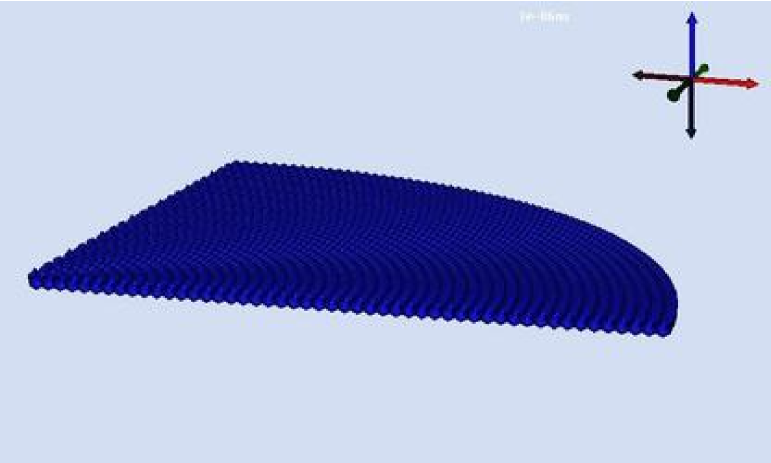
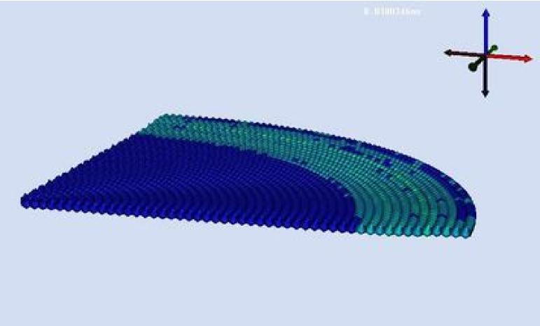
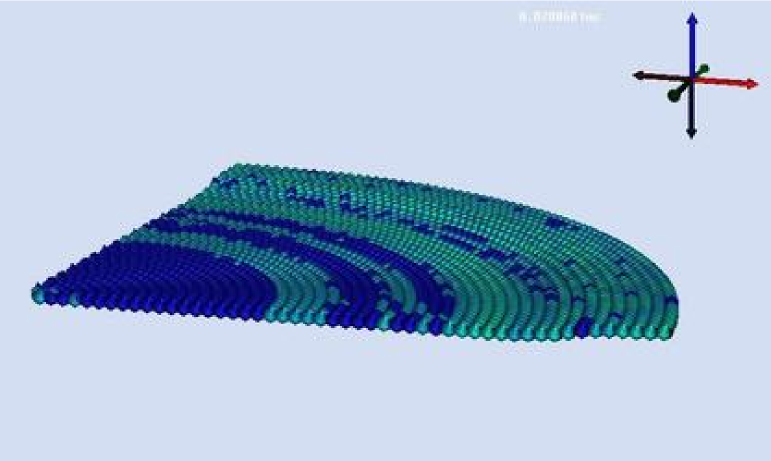
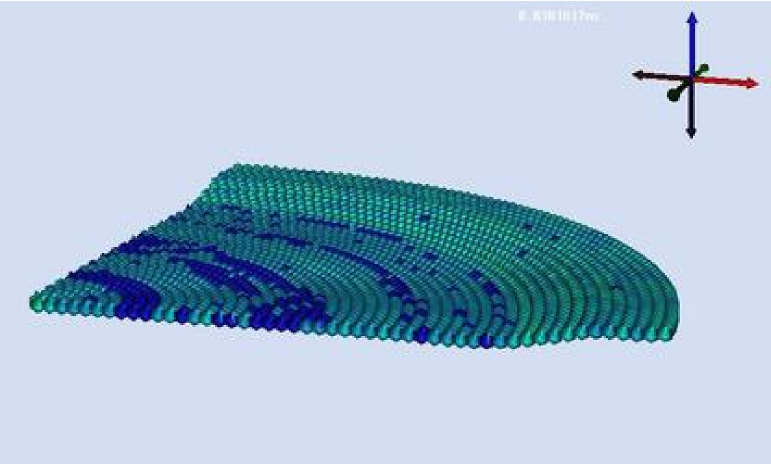
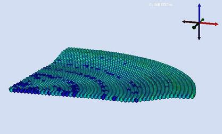
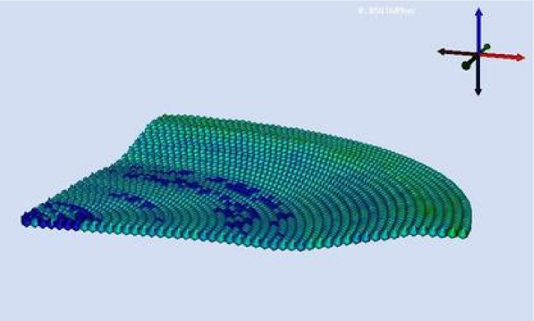
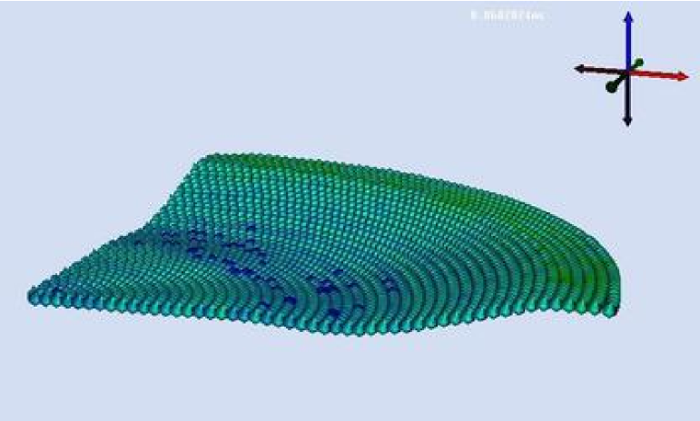
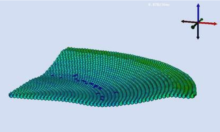
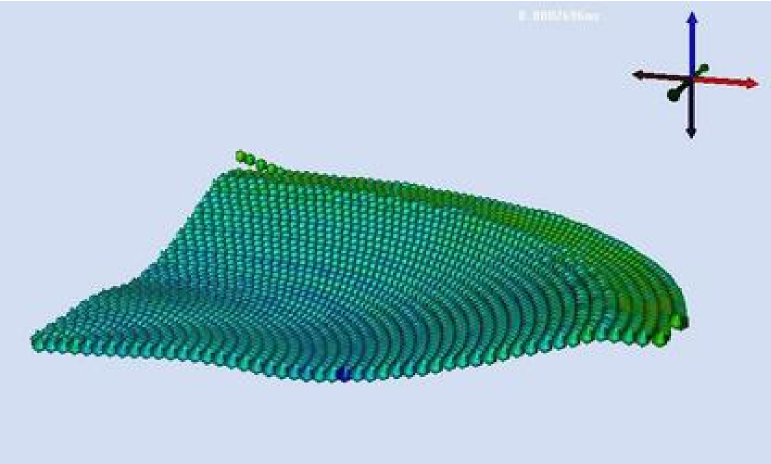
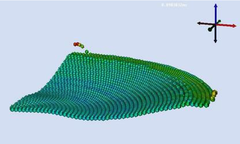
   Figure 1: Deformation of punched circular plane shell.

   Substantial deformation of the shell occurs before particles at the edges tend to tear off. The tearing off of particles is due to the presence of large rotation rates ($\mathbf{r}$) which are due to the stiffness of the rotational acceleration equation  (51). The implicit correction does not appear to be adequate beyond a certain point and a fully implicit shell formulation may be required for accurate simulation of extremely large deformations.

   Particles in the figure have been colored using the equivalent stress at the center-of-mass of the shell. The stress distribution in the shell is quite uniform, though some artifacts in the form of rings appear. An implicit formulation has been shown to remove such artifacts in the stress distribution in membranes [10]. Therefore, an implicit formulation may be useful for the shell formulation. Another possibility is that these artifacts may be due to membrane and shear locking, a known phenomenon in finite element formulations of shells based on a continuum approach [1, 11]. Such locking effects can be reduced using an addition hour glass control step [1] in the simulation.

2. Pinched Cylindrical Shell
   The pinched cylindrical shell is one of the benchmark problems proposed by MacNeal and Harder [12]. The cylindrical shell that has been simulated in this work has dimensions similar to those used by Li et al. [13]. The shell is pinched by contact with two small rigid solid cylinders placed diametrically opposite each other and located at the midpoint of the axis of the cylinder. Each of the solid cylinders is 0.25 cm in radius, 0.5 cm in length, and moves toward the center of the pinched shell in a radial direction at 10 ms^-1. The material of the shell is annealed copper (properties are shown in Table 1). The cylindrical shell is 2.5 cm in radius, 5.0 cm long, and 0.05 cm thick.

   Snapshots of the deformation of the pinched cylindrical shell are shown in Figure 2.

   

   

   

   

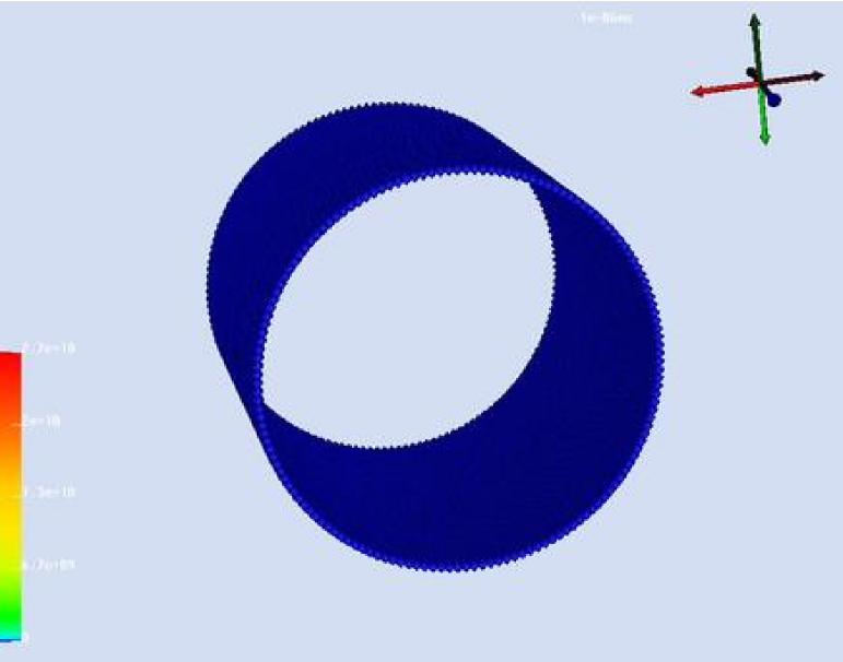
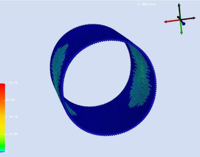
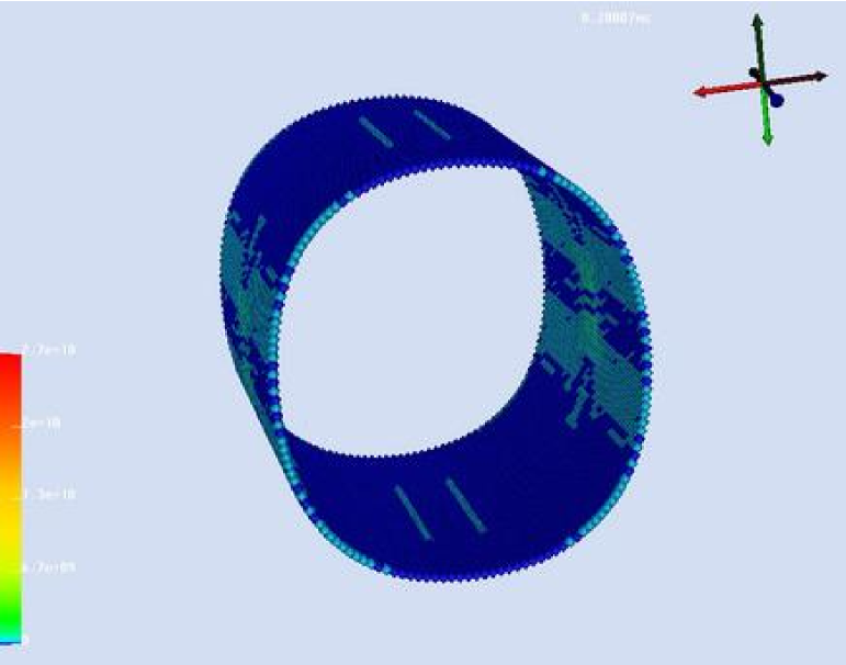
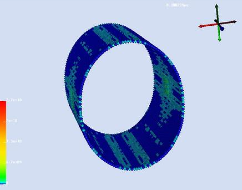
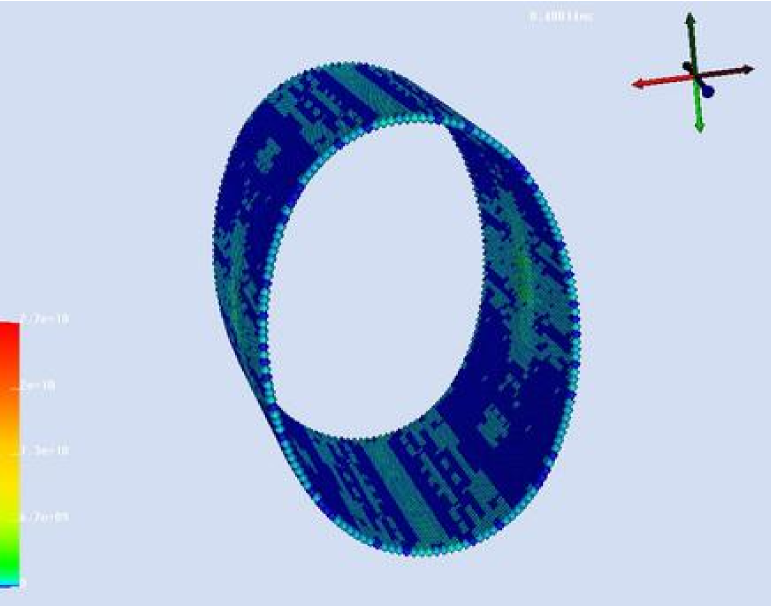
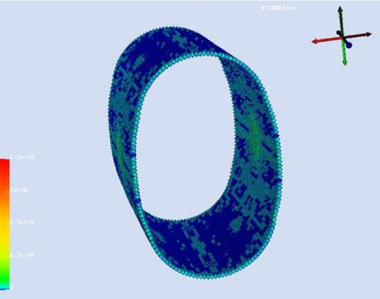
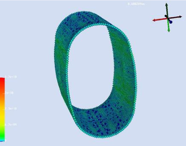
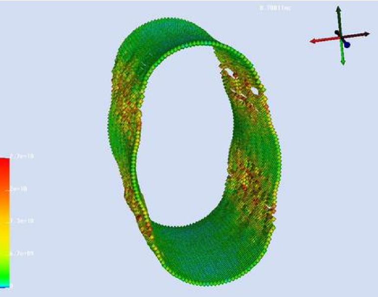
   Figure 2: Deformation of pinched cylindrical shell.

   The deformation of the shell proceeds uniformly for 60 ms. However, at this time the increments of rotation rate begin to increase rapidly at each time step, even though the velocity of the center-of-mass of the shell still remains stable. This effect can be attributed to the stiffness of the rotational inertia equation. The effect is that extremely large rotation rates are produced at 70 ms causing high velocities and eventual numerical fracture of the cylinder. The problem may be solved using an implicit shell formulation.

3. Inflating Spherical Shell
   The inflating spherical shell problem is similar to that used to model lipid bilayers by Ayton et al. [14]. The shell is made of a soft rubbery material with a density of 10 kg m^-3, a bulk modulus of 60 KPa and a shear modulus of 30 KPa. The sphere has a radius of 0.5 m and is 1 cm thick. The spherical shell is pressurized by an initial internal pressure of 10 KPa. The pressure increases in proportion to the internal surface area as the sphere inflates.

   The deformation of the shell with time is shown in Figure 3.

   

   

   

   

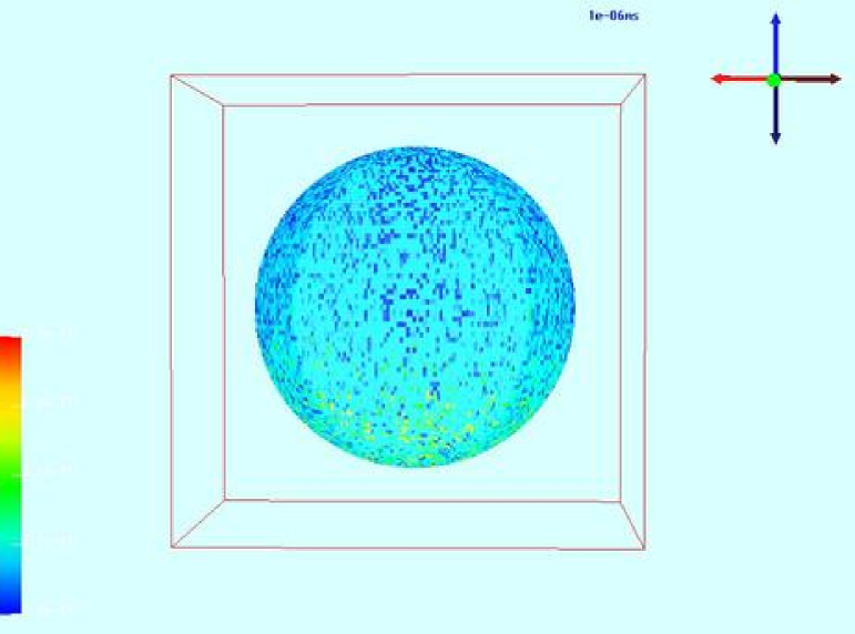
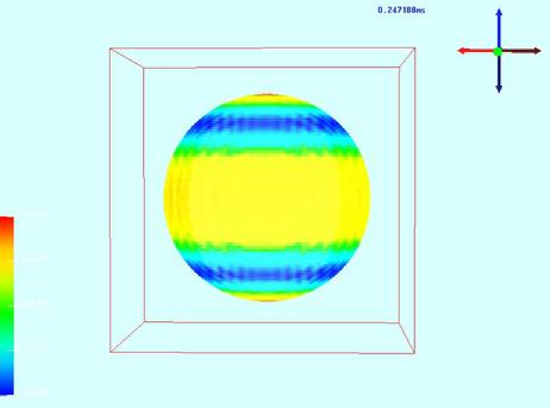
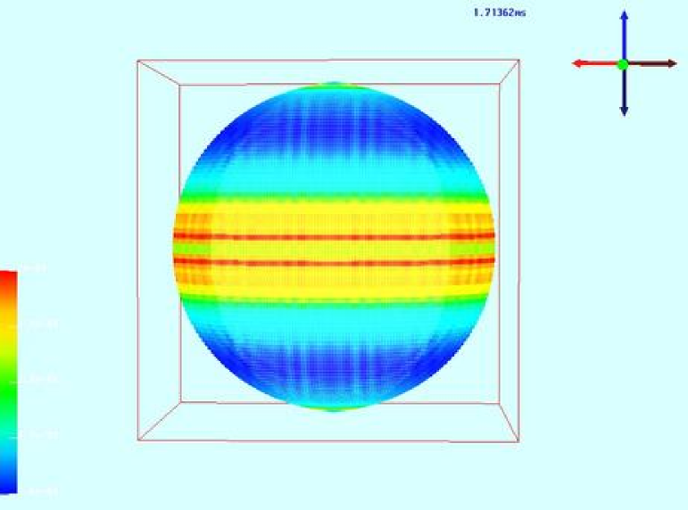
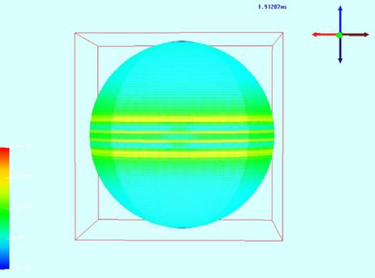
   Figure 3: Deformation of inflating spherical shell.

   The particles in the figure are colored on the basis of the equivalent stress. Though there is some difference between the values at different latitudes in the sphere, the equivalent stress is quite uniform in the shell. The variation can be reduced using the implicit material point method [15].

4 Summary

A shell formulation has been developed and implemented for the explicit time stepping material point method based on the work of Lewis et al. [2]. Three different shell geometries and loading conditions have been tested. The results indicate that the stiff nature of the equation for rotational inertia may require the use of an implicit time stepping scheme for shell materials.

References

- [1] T. Belytschko, W.K. Liu, and B. Moran. Nonlinear Finite Elements for Continua and Structures. John Wiley and Sons, Ltd., New York, 2000.
- [2] M.W. Lewis, B.A. Kashiwa, and R.M. Rauenzahn. Hydrodynamic ram modeling with the immersed boundary method. In Proc., ASME Pressure Vessels and Piping Conference, San Diego, California, 1998. American Society of Mechanical Engineers.
- [3] H.L. Schreyer. Lecture Notes in Plate Theory. University of New Mexico, Albuquerque, 1997.
- [4] D. Sulsky, Z. Chen, and H.L. Schreyer. A particle method for history dependent materials. Comput. Methods Appl. Mech. Engrg., 118:179–196, 1994.
- [5] S.G. Bardenhagen and E.M. Kober. The generalized interpolation material point method. submitted to Int. J. Numer. Meth. Engng., 2000.
- [6] S.G. Bardenhagen, J.U. Brackbill, and D. Sulsky. The material-point method for granular materials. Comput. Methods Appl. Mech. Engrg., 187:529–541, 2000.
- [7] S.G. Bardenhagen, J.E. Guilkey, K.M Roessig, J.U. BrackBill, W.M. Witzel, and J.C. Foster. An improved contact algorithm for the material point method and application to stress propagation in granular material. Computer Methods in the Engineering Sciences, 2(4):509–522, 2001.
- [8] J.C. Simo and T.J.R. Hughes. Computational Inelasticity. Springer-Verlag, New York, 1998.
- [9] B.A. Kashiwa and M.W Lewis. CFDLIB version 02.1. Los Alamos National Laboratories, Los Alamos, New Mexico, 2002.
- [10] J.E. Guilkey and J.A. Weiss. A general membrane formulation for use with the material point method. In preparation., 2002.
- [11] A. Libai and J. G. Simmonds. The Nonlinear Theory of Elastic Shells: 2nd Edition. Cambridge University Press, Cambridge, UK, 1998.
- [12] R.H. MacNeal and R.L. Harder. A proposed standard set of problems to test finite element accuracy. Finite Elements in Analysis and Design, 11:3–20, 1985.
- [13] S. Li, W. Hao, and W.K. Liu. Numerical simulations of large deformation of thin shell structures using meshfree methods. Computational Mechanics, 25(2-3):102–116, 2000.
- [14] G. Ayton, A.M. Smondyrev, S.G. Bardenhagen, P. McMurtry, and G.A. Voth. Interfacing molecular dynamics and macro-scale simulations for lipid bilayer vesicles. Biophysical Journal, 83:1026–1038, 2002.
- [15] J.E. Guilkey and J.A. Weiss. Implicit time integration for the material point method: Quantitative and algorithmic comparisons with the finite element method. Int. J. Numer. Meth. Engng. (in press), 2003.