Phase diagram of a dilute ferromagnet model with antiferromagnetic next-nearest-neighbor interactions

Abstract

We have studied the spin ordering of a dilute classical Heisenberg model with spin concentration $x$, and with ferromagnetic nearest-neighbor interaction $J_{1}$ and antiferromagnetic next-nearest-neighbor interaction $J_{2}$. Magnetic phases at absolute zero temperature $T=0$ are determined examining the stiffness of the ground state, and those at finite temperatures $T\neq 0$ are determined calculating the Binder parameter $g_{L}$ and the spin correlation length $\xi_{L}$. Three ordered phases appear in the $x-T$ phase diagram: (i) the ferromagnetic (FM) phase; (ii) the spin glass (SG) phase; and (iii) the mixed (M) phase of the FM and the SG. Near below the ferromagnetic threshold $x_{\rm F}$, a reentrant SG transition occurs. That is, as the temperature is decreased from a high temperature, the FM phase, the M phase and the SG phase appear successively. The magnetization which grows in the FM phase disappears in the SG phase. The SG phase is suggested to be characterized by ferromagnetic clusters. We conclude, hence, that this model could reproduce experimental phase diagrams of dilute ferromagnets Fe_xAu_1-x and Eu_xSr_1-xS.

I Introduction

Prototypes of spin glass (SG) are ferromagnetic dilute alloys such as Fe_xAu_1-xColes , Eu_xSr_1-xSMaletta1 ; Maletta2 and Fe_xAl_1-xShull ; Motoya . Those alloys have a common phase diagram as schematically shown in Fig. 1. It is shared with the ferromagnetic (FM) phase at higher spin concentrations and the SG phase at lower spin concentrations, together with the paramagnetic (PM) phase at high temperatures. A notable point is that a reentrant spin glass (RSG) transition occurs at the phase boundary between the FM phase and the SG phase. That is, as the temperature is decreased from a high temperature, the magnetization that grows in the FM phase vanishes at that phase boundary. The SG phase realized at lower temperatures is characterized by ferromagnetic clustersColes ; Maletta1 ; Maletta2 ; Motoya . A similar phase diagram has also been reported for amorphous alloys $(T_{1-x}T^{\prime}_{x})_{75}$B₆Al₃ with $T$ = Fe or Co and $T^{\prime}$ = Mn or NiYeshurun . It is believed that the phase diagram of Fig. 1 arises from the competition between ferromagnetic and antiferromagnetic interactions. For example, in Fe_xAu_1-x, the spins are coupled via the long-range oscillatory Ruderman-Kittel-Kasuya-Yoshida (RKKY) interaction. Also, in Eu_xSr_1-xS, the Heisenberg spins of $S=7/2$ are coupled via short-range ferromagnetic nearest-neighbor exchange interaction and antiferromagnetic next-nearest-neighbor interactionEuSrS . Nevertheless, the phase diagrams of the dilute alloys have not yet been understood theoretically. Several models have been proposed for explaining the RSG transitionSaslow ; Gingras1 ; Hertz . However, no realistic model has been revealed that reproduces itReger&Young ; Gingras2 ; Morishita . Our primary question is, then, whether the experimental phase diagrams with the RSG transition are reproducible using a simple dilute model with competing ferromagnetic and antiferromagnetic interactions.

Figure 1: A schematic phase diagram of a ferromagnetic dilute alloy.

This study elucidates a dilute Heisenberg model with competing short-range ferromagnetic nearest-neighbor exchange interaction $J_{1}$ and antiferromagnetic next-nearest-neighbor interaction $J_{2}$. This model was examined nearly 30 years ago using a computer simulation techniqueBinder at rather high spin concentrations and the phase boundary between the PM phase and the FM phase was obtained. However, the SG transition and the RSG transition have not yet been examined. Recent explosive advances in computer power have enabled us to perform larger scale computer simulations. Using them, we reexamine the spin ordering of the model for both $T=0$ and $T\neq 0$ in a wide-spin concentration range. Results indicate that the model reproduces qualitatively the experimental phase diagrams. In particular, we show that the model reproduces the RSG transition. A brief report of this result was given in Ref. 15.

The paper is organized as follows. In Sec. II, we present the model. In Sec. III, the ground state properties are discussed. We will determine threshold $x_{\rm F}$, above which the ground state magnetization remains finite. Then we examine the stabilities of the FM phase and the SG phase calculating excess energies that are obtained by twisting the ground state spin structure. Section IV presents Monte Carlo simulation results. We will give both the phase boundaries between the PM phase and the FM phase and between the PM phase and the SG phase. Immediately below $x=x_{\rm F}$, we find the RSG transition. Section V is devoted to our presentation of important conclusions.

II Model

We start with a dilute Heisenberg model with competing nearest-neighbor and next-nearest-neighbor exchange interactions described by the Hamiltonian:

$$H= - \sum_{\langle ij\rangle}^{nn}J_{1}x_{i}x_{j}\bm{S}_{i}\cdot\bm{S}_{j}+\sum_{\langle kl\rangle}^{nnn}J_{2}x_{k}x_{l}\bm{S}_{k}\cdot\bm{S}_{l},$$ (1)

where $\bm{S}_{i}$ is the classical Heisenberg spin of $|\bm{S}_{i}|=1$; $J_{1}(>0)$ and $J_{2}(>0)$ respectively represent the nearest-neighbor and the next-nearest-neighbor exchange interactions; and $x_{i}=1$ and 0 when the lattice site $i$ is occupied respectively by a magnetic and non-magnetic atom. The average number of $x(\equiv\langle x_{i}\rangle)$ is the concentration of a magnetic atom. Note that an experimental realization of this model is Eu_xSr_1-xSEuSrS , in which magnetic atoms (Eu) are located on the fcc lattice sites. Here, for simplicity, we consider the model on a simple cubic lattice with $J_{2}=0.2J_{1}$Model .

III Magnetic Phase at $T=0$

We consider the magnetic phase at $T=0$. Our strategy is as follows. First we consider the ground state of the model on finite lattices for various spin concentrations $x$. Examining the size dependence of magnetization $M$, we determine the spin concentration $x_{\rm F}$ above which the magnetization will take a finite, non-vanishing value for $L\rightarrow\infty$. Then we examine the stability of the ground state by calculating twisting energies. We apply a hybrid genetic algorithm (HGA)GA for searching for the ground state.

III.1 Magnetization $M$ at $T=0$

We treat lattices of $L\times L\times L$ with periodic boundary conditions. The ground state magnetizations $\bm{M}_{L}^{\rm G}(\equiv\sum_{i}x_{i}\bm{S}_{i})$ are calculated for individual samples and averaged over the samples. That is, $M=[|\bm{M}_{L}^{\rm G}|]$, where $[\cdots]$ represents a sample average. Numbers $N_{s}$ of samples with different spin distributions are $N_{s}=1000$ for $L\leq 8$, $N_{s}=500$ for $10\leq L\leq 14$, and $N_{s}=64$ for $L\geq 16$. We apply the HGA with the number $N_{p}$ of parents of $N_{p}=16$ for $L\leq 8$, $N_{p}=64$ for $L=10$, $N_{p}=128$ for $L=12$, $\dots$, and $N_{p}=512$ for $L\geq 16$.

Figure 2: Ground state magnetizations $M$ in $L\times L\times L$ lattices for various spin concentrations $x$.

Figure 3: Binder parameter $g_{L}$ at $T=0$ in $L\times L\times L$ lattices for various spin concentrations $x$.

Figure 2 portrays plots of magnetization $M$ as a function of $L$ for various spin concentrations $x$. A considerable difference is apparent in the $L$-dependence of $M$ between $x\leq 0.82$ and $x\geq 0.84$. For $x\leq 0.82$, as $L$ increases, $M$ decreases exponentially revealing that $M\rightarrow 0$ for $L\rightarrow\infty$. On the other hand, for $x\geq 0.84$, $M$ decreases rather slowly, suggesting that $M$ remains finite for $L\rightarrow\infty$.

To examine the above suggestion, we calculate the Binder parameter $g_{L}$BinderP defined as

$$g_{L}=(5-3\frac{[|\bm{M}_{L}^{\rm G}|^{4}]}{[|\bm{M}_{L}^{\rm G}|^{2}]^{2}})/2.$$ (2)

When the sample dependence of $\bm{M}_{L}^{\rm G}$ vanishes for $L\rightarrow\infty$, $g_{L}$ increases with $L$ and becomes unity. That is, if the system has its magnetization inherent in the system, $g_{L}$ increases with $L$. On the other hand, $g_{L}\rightarrow 0$ for $L\rightarrow\infty$ when $\bm{M}_{L}^{\rm G}$ tends to scatter according to a Gaussian distribution. Figure 3 represents the $L$-dependence of $g_{L}$ for various $x$. For $x\leq 0.82$, as $L$ increases, $g_{L}$ increases and subsequently becomes maximum at $L\sim 8$, decreasing thereafter. This fact reveals that the FM phase is absent for $x\leq 0.82$. For $x\geq 0.84$, a decrease is not apparent. In particular, $g_{L}$ for $x\geq 0.86$ increases gradually toward 1, indicating that the FM phase occurs for $L\rightarrow\infty$. We suggest, hence, the threshold of the FM phase of $x_{\rm F}=0.84\pm 0.02$ at $T=0$.

III.2 Stiffness of the ground state

The next question is, for $x>x_{\rm F}$, whether or not the FM phase is stable against a weak perturbation. Also, for $x<x_{\rm F}$, whether or not some frozen spin structure occurs. To consider these problems, we examine the stiffness of the ground stateEndoh1 ; Endoh2 .

We briefly present the methodEndoh1 . We consider the system on a cubic lattice with $L\times L\times(L+1)$ lattice sites in which the $z$-direction is chosen as one for $(L+1)$ lattice sites. That is, the lattice is composed of $(L+1)$ layers with $L\times L$ lattice sites. Periodic boundary conditions are applied for every layer and an open boundary condition to the $z$-direction. Therefore, the lattice has two opposite surfaces: $\Omega_{1}$ and $\Omega_{L+1}$. We call this system as the reference system. First, we determine the ground state of the reference system. We denote the ground state spin configuration on the $l$th layer as $\{\bm{S}_{l,i}\}\ (l=1$ – $(L+1))$ and the ground state energy as $E_{L}^{\rm G}$. Then we add a distortion inside the system in such a manner that, under a condition that $\{\bm{S}_{1,i}\}$ are fixed, $\{\bm{S}_{L+1,i}\}$ are rotated by the same angle $\phi$ around some common axis. We also call this system a twisted system. The minimum energy $E_{L}(\phi)$ of the twisted system is always higher than $E_{L}^{\rm G}$. The excess energy $\Delta E_{L}(\phi)(\equiv E_{L}(\phi)-E_{L}^{\rm G})$ is the net energy that is added inside the lattice by this twist, because the surface energies of $\Omega_{1}$ and $\Omega_{L+1}$ are conserved. The stiffness exponent $\theta$ may be defined by the relation $\Delta E_{L}(\phi)\propto L^{\theta}$Comm_Endoh . If $\theta>0$, the ground state spin configuration is stable against a small perturbation. That is, the ground state phase will occur at least at very low temperatures. On the other hand, if $\theta<0$, the ground state phase is absent at any non-zero temperature.

To apply the above idea to our model, we must give special attention to the rotational axis for $\{\bm{S}_{L+1,i}\}$ because the reference system has a non-vanishing magnetization ${\bm{M}}_{L}^{G}$. For the following arguments, we separate each spin ${\bm{S}}_{l,i}$ into parallel and perpendicular components:

$$\left\{\begin{array}[]{l}{\bm{S}}_{l,i}^{\parallel}=({\bm{S}}_{l,i}\cdot{\bm{m}}){\bm{m}}\\ {\bm{S}}_{l,i}^{\perp}=({\bm{S}}_{l,i}\times{\bm{m}})\times{\bm{m}},\end{array}\right.$$

where ${\bm{m}}={\bm{M}}_{L}^{\rm G}/|{\bm{M}}_{L}^{\rm G}|$. We consider two twisted systems. One is a system in which $\{\bm{S}_{L+1,i}^{\perp}\}$ are rotated around the axis that is parallel to the magnetization ${\bm{M}}_{L}^{\rm G}$. We denote the minimum energy of this twisted system as $E_{L}^{\perp}(\phi)$. The other is a system in which $\{\bm{S}_{L+1,i}\}$ are rotated around an axis that is perpendicular to ${\bm{M}}_{L}^{\rm G}$. We also denote the minimum energy of this twisted system as $E_{L}^{\parallel}(\phi)$. Note that, in this twisted system, $\{{\bm{S}}_{l,i}^{\parallel}\}$ mainly change, but $\{{\bm{S}}_{l,i}^{\perp}\}$ also change. Choices in the rotation axis are always possible in finite systems, even when $x<x_{\rm F}$ because a non-vanishing magnetization (${\bm{M}}_{L}^{\rm G}\neq 0$) exists in the Heisenberg model on a finite lattice. Of course the difference between $E_{L}^{\perp}(\phi)$ and $E_{L}^{\parallel}(\phi)$ will diminish for $L\rightarrow\infty$ in the range $x<x_{\rm F}$. The excess energies $\Delta E_{L}^{\perp}(\phi)$ and $\Delta E_{L}^{\parallel}(\phi)$ in our model are given as

$$\Delta E_{L}^{\perp}(\phi) = [E_{L}^{\perp}(\phi)-E_{L}^{\rm G}],$$ (3)

$$\Delta E_{L}^{\parallel}(\phi) = [E_{L}^{\parallel}(\phi)-E_{L}^{\rm G}],$$ (4)

with $[\cdots]$ being the sample average.

We calculated $\Delta E_{L}^{\perp}(\phi)$ and $\Delta E_{L}^{\parallel}(\phi)$ for a common rotation angle of $\phi=\pi/2$ in lattices of $L\leq 14$. Numbers of the samples are $N_{s}\sim 1000$ for $L\leq 10$ and $N_{s}\sim 250$ for $L=12$ and 14. Hereafter we simply describe $\Delta E_{L}^{\perp}(\pi/2)$ and $\Delta E_{L}^{\parallel}(\pi/2)$ respectively as $\Delta E_{L}^{\perp}$ and $\Delta E_{L}^{\parallel}$. Figures 4(a) and 4(b) respectively show lattice size dependences of $\Delta E_{L}^{\perp}$ and $\Delta E_{L}^{\parallel}$ for $x<x_{\rm F}$ and $x>x_{\rm F}$. We see that, for all $x$, $\Delta E_{L}^{\parallel}>\Delta E_{L}^{\perp}$ and both increase with $L$. When $x<x_{\rm F}$, as expected, the difference between $\Delta E_{L}^{\perp}$ and $\Delta E_{L}^{\parallel}$ diminishes as $L$ increases.

Figure 4: Excess energies $\Delta E_{L}^{\perp}$ and $\Delta E_{L}^{\parallel}$ for $L\times L\times(L+1)$ lattices for various spin concentrations: (a) $x<x_{\rm F}$ and (b) $x>x_{\rm F}$. Open symbols represent $\Delta E_{L}^{\perp}$ and filled symbols $\Delta E_{L}^{\parallel}$. Symbols $\times$ in (a) represent the averages of those values.

Now we discuss the stability of the spin configuration. First we consider the stability of $\{{\bm{S}}_{l,i}^{\parallel}\}$, i.e., the stability of the FM phase. In the pure FM case ($x=1$), ${\bm{S}}_{l,i}^{\perp}=0$ and $\Delta E_{L}^{\parallel}$ gives the net excess energy for the twist of the magnetization. This is not the same in the case of ${\bm{S}}_{l,i}^{\perp}\neq 0$. Because the twist in $\{{\bm{S}}_{l,i}^{\parallel}\}$ accompanies the change in $\{{\bm{S}}_{l,i}^{\perp}\}$, $\Delta E_{L}^{\parallel}$ does not give the net excess energy for the twist of $\{{\bm{S}}_{l,i}^{\parallel}\}$. For that reason, we consider the difference $\Delta E_{L}^{\rm F}$ between the two excess energies:

$$\Delta E_{L}^{\rm F}=\Delta E_{L}^{\parallel}-\Delta E_{L}^{\perp}.$$ (5)

If $\Delta E_{L}^{\rm F}\rightarrow\infty$ for $L\rightarrow\infty$, the FM phase will be stable against a small perturbation. We define the stiffness exponent $\theta^{\rm F}$ of the FM phase as

$$\Delta E_{L}^{\rm F}\propto L^{\theta^{\rm F}}.$$ (6)

Figure 5 shows $\Delta E_{L}^{\rm F}$ for $x\geq 0.80$. We have $\theta^{\rm F}>0$ for $x\geq 0.85$ and $\theta^{\rm F}<0$ for $x=0.80$. These facts show that, in fact, the FM phase is stable for $x>x_{\rm F}\sim 0.84$ at $T\sim 0$.

Figure 5: Difference in the excess energy $\Delta E_{L}^{F}=\Delta E_{L}^{\parallel}-\Delta E_{L}^{\perp}$ for $L\times L\times(L+1)$ lattice for various spin concentrations $x$.

Next, we consider the stability of the transverse components $\{{\bm{S}}_{l,i}^{\perp}\}$. Hereafter we call the phase with $\{{\bm{S}}_{l,i}^{\perp}\neq 0\}$ a SG phase. For $x<x_{\rm F}$, we may examine the stiffness exponent $\theta^{\rm SG}$ using either $\Delta E_{L}^{\perp}$ or $\Delta E_{L}^{\parallel}$. Here we estimate its value using an average value of them. For $x>x_{\rm F}$, we examine it using $\Delta E_{L}^{\perp}$. In this range of $x$, meticulous care should be given to a strong finite size effectComm_finite . We infer that this finite size effect for $x>x_{\rm F}$ is attributable to a gradual decrease in the magnetization ${\bm{M}}$ for finite $L$ (see Fig. 2). That is, the magnitude of the transverse component $|{\bm{S}}_{l,i}^{\perp}|$ will gradually increase with $L$, which will engender an additional increase of $\Delta E_{L}^{\perp}$ as $L$ increases. This increase of $|{\bm{S}}_{l,i}^{\perp}|$ will cease for $L\rightarrow\infty$. Consequently, we estimate the value of $\theta^{\rm SG}$ from the relations:

$$(\Delta E_{L}^{\parallel}+\Delta E_{L}^{\perp})/2 \propto L^{\theta^{\rm SG}}\ \ \ {\rm for}\ \ \ \ x<x_{\rm F},$$ (7)

$$\Delta E_{L}^{\perp}/|{\bm{S}}^{\perp}|^{2} \propto L^{\theta^{\rm SG}}\ \ \ {\rm for}\ \ \ \ x>x_{\rm F},$$ (8)

where $|{\bm{S}}^{\perp}|^{2}=1-|{\bm{M}}/xN|^{2}$. Log-log plots of those quantities versus $L$ are presented in Fig. 4(a) for $x<x_{\rm F}$ and in Fig. 6 for $x>x_{\rm F}$. We estimate $\theta^{\rm SG}$ using data for $L\geq 8$ and present the results in the figures. Note that for $x>0.90$, studies of bigger lattices will be necessary to obtain a reliable value of $\theta^{\rm SG}$ because $\Delta E_{L}^{\perp}$ for $L\lesssim 14$ is too small to examine the stiffness of $\{{\bm{S}}_{l,i}^{\perp}\}$.

Figure 7 shows stiffness exponents $\theta^{\rm F}$ and $\theta^{\rm SG}$ as functions of $x$. As $x$ increases, $\theta^{\rm SG}$ changes its sign from negative to positive at $x_{SG}=0.175\pm 0.025$. This value of $x_{\rm SG}$ is close to the percolation threshold of $x_{\rm p}\sim 0.137$Essam . Above $x_{\rm SG}$, $\theta^{\rm SG}$ takes almost the same value of $\theta^{\rm SG}\sim 0.75$ up to $x\sim 0.9$. On the other hand, $\theta^{\rm F}$ changes its sign at $x_{\rm F}\sim 0.84$ and increases toward $\theta^{\rm F}=1$ at $x=1$. A notable point is that $\theta^{\rm SG}>0$ for $x>x_{\rm F}$. That is, a mixed (M) phase of the ferromagnetism and the SG phase will occur for $x>x_{\rm F}$ at $T=0$. We could not estimate another threshold of $x$ above which the purely FM phase is realized.

Figure 6: The normalized excess energy $\Delta E_{L}^{\perp}/|{\bm{S}}^{\perp}|^{2}$ for $L\times L\times(L+1)$ lattices for various spin concentrations $x>x_{\rm F}$.

Figure 7: Stiffness exponents $\theta^{\rm SG}$ and $\theta^{\rm F}$ for various spin concentrations $x$. Here, we remove $\theta^{\rm SG}$ at $x=0.95$.

IV Monte Carlo Simulation

We next consider the magnetic phase at finite temperatures using the MC simulation technique. We make a MC simulation for $x\geq 0.20$. We treat lattices of $L\times L\times L\ (L=8-48)$ with periodic boundary conditions. Simulation is performed using a conventional heat-bath MC method. The system is cooled gradually from a high temperature (cooling simulation). For larger lattices, $200000$ MC steps (MCS) are allowed for relaxation; data of successive $200000$ MCS are used to calculate average values. We will show later that these MCS are sufficient for studying equilibrium properties of the model at a temperature range within which the RSG behavior is found. Numbers $N_{s}$ of samples with different spin distributions are $N_{s}=1000$ for $L\leq 16$, $N_{s}=500$ for $L=24$, $N_{s}=200$ for $L=32$, and $N_{s}=80$ for $L=48$. We measure the temperature in units of $J_{1}$ ($k_{\rm B}=1$).

IV.1 Thermal and magnetic properties

We calculate the specific heat $C$ and magnetization $M$ given by

$$C = \frac{1}{T^{2}}([\langle E(s)^{2}\rangle]-[\langle E(s)\rangle^{2}]),$$ (9)

$$M = [\langle M(s)\rangle].$$ (10)

Therein, $E(s)$ and $M(s)(\equiv|\sum_{i}x_{i}\bm{S}_{i}|)$ represent the energy and magnetization at the $s$th MC step, and $N$ is the number of the lattice sites. Here $\langle\cdots\rangle$ represents an MC average.

Figure 8: Specific heats $C$ in the $32\times 32\times 32$ lattice for various spin concentrations $x$.

Figure 9: Magnetizations $M$ in the $32\times 32\times 32$ lattice for various spin concentrations $x$.

Figure 8 shows the specific heat $C$ for various concentrations $x$. For $x\geq 0.90$, $C$ exhibits a sharp peak at a high temperature, revealing that a FM phase transition occurs at that temperature. As $x$ decreases, the peak broadens. On the other hand, at $x\sim 0.85$ a hump is apparent at a lower temperature; it grows with decreasing $x$. This fact implies that, for $x\lesssim 0.85$, another change in the spin structure occurs at a lower temperature. As $x$ decreases further, the broad peak at a higher temperature disappears and only a single broad peak is visible at a lower temperature.

Figure 9 shows temperature dependencies of magnetization $M$ for various $x$. For $x=1$, as the temperature decreases, $M$ increases rapidly below the temperature, revealing the occurrence of a FM phase. As $x$ decreases, $M$ exhibits an interesting phenomenon: in the range of $0.78\lesssim x\lesssim 0.85$, $M$ once increases, reaches a maximum value, then decreases. We also perform a complementary simulation to examine this behavior of $M$. That is, starting with a random spin configuration at a low temperature, the system is heated gradually (heating simulation). Figure 10 shows temperature dependencies of $M$ for $x=0.80$ in both cooling and heating simulations for various $L$. For $T\gtrsim 0.1J_{1}$, data of the two simulations almost coincide mutually, even for large $L$. We thereby infer that $M$ for $T\gtrsim 0.1J_{1}$ are of thermal equilibrium and the characteristic behavior of $M$ found here is an inherent property of the model. For $T<0.1J_{1}$, a great difference in $M$ is apparent between the two simulations; estimation of the equilibrium value is difficult. We speculate, however, that the heating simulation gives a value of $M$ that is similar to that in the equilibrium state because the data in the heating simulation seem to concur with those obtained in the ground state.

Figure 10 shows the remarkable lattice size dependence of $M$. For smaller $L$, as the temperature decreases, $M$ decreases slightly at very low temperatures. The decrease is enhanced as $L$ increases. Consequently, a strong size-dependence of $M$ is indicated for $T\lesssim 0.1J_{1}$. These facts suggest that $M$ for $L\rightarrow\infty$ disappears at low temperatures as well as at high temperatures. The next section presents an examination of this issue, calculating the Binder parameter.

Figure 10: Magnetizations $M$ for $x=0.80$ in the $L\times L\times L$ lattice. Open symbols indicate $M$ in the cooling simulation and filled symbols indicate that in the heating simulation. Data at $T=0$ indicate those in the ground state given in Fig. 2.

IV.2 Ferromagnetic phase transition

The Binder parameter $g_{L}$ at finite temperatures is defined as

$$g_{L}=(5-3\frac{[\langle M(s)^{4}\rangle]}{[\langle M(s)^{2}\rangle]^{2}})/2.$$ (11)

We calculate $g_{L}$ for various $x$. Figures 11(a)–11(d) show $g_{L}$’s for $x\sim x_{\rm F}$Comm_gL . In fact, $g_{L}$ for $x<x_{\rm F}$ exhibits a novel temperature dependence. As the temperature is decreased from a high temperature, $g_{L}$ increases rapidly, becomes maximum, then decreases. In particular, we see in Fig. 11(b) for $x=0.80$ $g_{L}$’s for different $L$ cross at two temperatures $T_{\rm C}$ and $T_{\rm R}$ ($<T_{\rm C}$). The cross at $T_{\rm C}/J_{1}\sim 0.26$ is a usual one that is found in the FM phase transition. That is, for $T>T_{\rm C}$, $g_{L}$ for a larger size is smaller than that for a smaller size; for $T<T_{\rm C}$, this size dependence in $g_{L}$ is reversed. On the other hand, the cross at $T_{\rm R}$ is strange: for $T<T_{\rm R}$, $g_{L}$ for a larger size again becomes smaller than that for a smaller size. Interestingly, the cross for different $g_{L}$ occur at almost the same temperature of $T_{\rm R}/J_{1}\sim 0.13$. These facts reveal that, as the temperature is decreased to below $T_{\rm R}$, the FM phase, which occurs below $T_{\rm C}$, disappears. Similar properties are apparent for $x=$ 0.79–0.82.

Figure 11: Binder parameters $g_{L}$ for various $x$. The $T_{\rm R}$ for $x=0.82$ was estimated by extrapolations of data obtained at higher temperatures.

IV.3 Spin glass phase transition

Figure 12: The SG correlation length $\xi_{L}$ divided by $L$ at different $x$. Insets show typical examples of the scaling plot.

Is the SG phase realized at low temperatures? A convincing way of examining the SG phase transition is a finite size scaling analysis of the correlation length, $\xi_{L}$, of different sizes $L$Ballesteros ; Lee . Data for the dimensionless ratio $\xi_{L}/L$ are expected to intersect at the SG transition temperature of $T_{\rm SG}$. Here we consider the correlation length of the SG component of the spin, i.e., $\tilde{\bm{S}}_{i}(\equiv{\bm{S}}_{i}-{\bm{m}})$ with ${\bm{m}}$ as the ferromagnetic component of ${\bm{m}}=\sum_{i}x_{i}{\bm{S}}_{i}/(xN)$. We perform a cooling simulation of a two-replica system with $\{{\bm{S}}_{i}\}$ and $\{{\bm{T}}_{i}\}$Bhatt . The SG order parameter, generalized to wave vector ${\bm{k}}$, $q^{\mu\nu}(\bm{k})$, is defined as

$$q^{\mu\nu}(\bm{k})=\frac{1}{xN}\sum_{i}\tilde{S}_{i}^{\mu}\tilde{T}_{i}^{\nu}e^{i{\bm{k}}{\bm{R}}_{i}},$$ (12)

where $\mu,\nu=x,y,z$. From this,the wave vector dependent SG susceptibility $\chi_{\rm SG}({\bm{k}})$ is determinate as

$$\chi_{\rm SG}({\bm{k}})=xN\sum_{\mu,\nu}[\langle|q^{\mu\nu}(\bm{k})|^{2}\rangle].$$ (13)

The SG correlation length can then be calculated from

$$\xi_{L}=\frac{1}{2\sin(k_{\rm min}/2)}(\frac{\chi_{SG}(0)}{\chi_{SG}({\bm{k}}_{\rm min})}-1)^{1/2},$$ (14)

where ${\bm{k}}_{\rm min}=(2\pi/L,0,0)$. It is to be noted that, in the FM phase (${\bm{m}}\neq 0$ for $L\rightarrow\infty$), the FM component will interfere with the development of the correlation length of the SG component $\tilde{\bm{S}}_{i}$. Then in that case we consider the transverse components $\tilde{\bm{S}}_{i}^{\perp}(\equiv(\tilde{\bm{S}}_{i}\times{\bm{m}})\times{\bm{m}})$ in eq. (13) instead of $\tilde{\bm{S}}_{i}$. The correlation length obtained using $\tilde{\bm{S}}_{i}^{\perp}$ is denoted as $\xi_{L}^{\perp}$.

We calculate $\xi_{L}/L$ or $\xi_{L}^{\perp}/L$ for $0.20\leq x\leq 0.90$. The crosses for different $L$ are found for $0.30\leq x\leq 0.90$. Figures 12(a)–12(c) show results of the temperature dependence of $\xi_{L}/L$ for typical $x$. Assuming that the SG transition occurs at the crossing temperature, we can scale all the data for each $x$ (see insets). For $x=0.20$, the crosses were not visible down to $T/J_{1}=0.02$. However, we can scale all the data assuming a finite transition temperature of $T_{\rm SG}/J_{1}\sim 0.01$. Thereby, we infer that the SG transition occurs for $0.20\lesssim x\lesssim 0.90$. This finding is compatible with the argument in the previous section that $\theta^{\rm SG}>0$ for $0.20\lesssim x\lesssim 0.90$.

It is noteworthy that the SG phase transition for ${\bm{m}}\neq 0$ is one in which the transverse spin components $\{\tilde{\bm{S}}_{i}^{\perp}\}$ order. Therefore we identify this phase transition as a Gabay and Toulouse (GT) transitionGT and the low temperature phase as a mixed (M) phase of the FM and a transverse SG. It is also noteworthy that, for $x=0.79$ and $x=0.80$, we estimate respectively $T_{\rm SG}/J_{1}=0.10\pm 0.01$ and $T_{\rm SG}/J_{1}=0.098\pm 0.005$, whereas respectively $T_{\rm R}/J_{1}=0.15\pm 0.01$ and $T_{\rm R}/J_{1}=0.125\pm 0.005$Comm_Error . These facts suggest that, as the temperature is decreased, the SG transition occurs after the disappearance of the FM phase ($T_{\rm SG}<T_{\rm R}$). The difference in transition temperatures of $T_{\rm INV}(\equiv T_{\rm R})$ and $T_{\rm SG}$ were reported in Fe_0.7Al_0.3Motoya . However, further studies are necessary to resolve this point because the treated lattices of $L\leq 20$ for estimating $T_{\rm SG}$ are not sufficiently large.

V Phase diagram

Figure 13: The phase diagram of the dilute Heisenberg model. Four arrows indicate, from the left to the right, the percolation threshold $x_{\rm p}$, the lower threshold of the SG phase $x_{\rm SG}$, the threshold of the ferromagnetic phase at finite temperatures $x_{\rm FT}$, and the ferromagnetic threshold at $T=0$, $x_{\rm F}$.

(a) $x=0.70$                            (b) $x=0.80$                            (c) $x=0.85$
                       

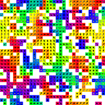
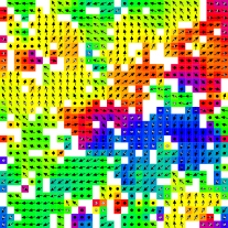
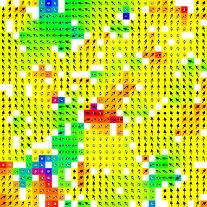
Figure 14: (Color online) Spin structures of the model for different $x$ at $T/J_{1}=0.04$ on a plane of the $32\times 32\times 32$ lattice. Spins represented here are those averaged over 10000 MCS. The positions of the non-magnetic atoms are represented in white.

Figure 13 shows the phase diagram of the model obtained in this study. It is shared by four phases: (i) the PM phase, (ii) the FM phase, (iii) the SG phase, and (iv) the M phase. A point that demands re-emphasis is that, just below the $T=0$ phase boundary between the SG phase and the M phase $(x_{\rm FT}<x<x_{\rm F})$, the RSG transition is found. This phase diagram is analogous with those observed in dilute ferromagnets Fe_xAu_1-xColes and Eu_xSr_1-xSMaletta1 ; Maletta2 . In particular, the occurrence of the mixed phase was reported in Fe_xAu_1-x.

We examine the low temperature spin structure. Figures 14(a) and 14(b) represent the spin structure in the SG phase ($x<x_{\rm F})$. We can see that the system breaks up to yield ferromagnetic clusters. In particular, for $x\lesssim x_{\rm F}$ (Fig. 14(b)), the cluster size is remarkable. Therefore the SG phase for $x\lesssim x_{\rm F}$ is characterized by ferromagnetic clusters with different spin directions. Figure 14(c) represents the spin structure in the M phase ($x>x_{\rm F})$. We can see that a ferromagnetic spin correlation extends over the lattice. There are ferromagnetic clusters in places. The spin directions of those clusters tilt to different directions. That is, as noted in the previous section, the M phase is characterized by the coexistance of the ferromagnetic long-range order and the ferromagnetic clusters with transverse spin component. The occurrence of ferromagnetic clusters at $x\sim x_{\rm F}$ are compatible with experimental observationsColes ; Maletta1 ; Maletta2 ; Motoya ; Yeshurun .

VI Conclusion

This study examined the phase diagram of a dilute ferromagnetic Heisenberg model with antiferromagnetic next-nearest-neighbor interactions. Results show that the model reproduces experimental phase diagrams of dilute ferromagnets. Moreover, the model was shown to exhibit reentrant spin glass (RSG) behavior, the most important issue. Other important issues remain unresolved, especially in the RSG transition. Why does the magnetization, which grows at high temperatures, diminish at low temperatures? Why does the spin glass phase transition take place after the disappearance of the ferromagnetic phase? We intend the model presented herein as one means to solve those and other remaining problems.

The authors are indebted to Professor K. Motoya for directing their attention to this problem of the RSG transition and for his valuable discussions. The authors would like to thank Professor T. Shirakura and Professor K. Sasaki for their useful suggestions. This work was financed by a Grant-in-Aid for Scientific Research from the Ministry of Education, Culture, Sports, Science and Technology.

References

- (1) B. R. Coles, B. V. Sarkissian, and R. H. Taylor, Phil. Mag. B 37, 489 (1978).
- (2) H. Malleta and P. Convert, Phys. Rev. Lett. 42, 108 (1979).
- (3) H. Maletta, G. Aeppli, and S. M. Shapiro, Phys. Rev. Lett. 48, 1490 (1982).
- (4) R. D. Shull, H. Okamoto, and P. A. Beck, Solid State Commun. 20, 863 (1976).
- (5) K. Motoya, S. M. Shapiro, and Y. Muraoka, Phys. Rev. B 28, 6183 (1983).
- (6) For example, Y. Yeshurun, M. B. Salamon, K. V. Rao, and H. S. Chen, Phys. Rev. B 24, 1536 (1981); and references therein.
- (7) H. Maletta and W. Felsch, Phys. Rev. B 20, 1245 (1979).
- (8) W. M. Saslow and G. Parker, Phys. Rev. Lett. 56, 1074 (1986).
- (9) M. J. P. Gingras and E. S. Sørensen, Phys. Rev. B 57, 10264 (1998).
- (10) J. A. Hertz, D. Sherrington, and Th. M. Nieuwenhuizen, Phys. Rev. E 60, R2460 (1999).
- (11) J. D. Reger and A. P. Young, J. Phys.: Condens. Matter 1, 915 (1989).
- (12) M. J. P. Gingras and E. S. Sørensen, Phys. Rev. B 46, 3441 (1992); and references therein.
- (13) F. Matsubara, K. Morishita, and S. Inawashiro, J. Phys. Soc. Jpn. 63, 416 (1994); and references therein.
- (14) K. Binder, W. Kinzel, and D. Stauffer, Z. Physik B 36, 161 (1979).
- (15) S. Abiko, S. Niidera, and F. Matsubara, Phys. Rev. Lett. 94, 227202 (2005).
- (16) Coordination numbers of the nearest and the next-nearest neighbor lattice sites are and in the fcc lattice, and and in the sc lattice. In that case, we choose the smaller ratio of instead of in EuxSr1-xS.
- (17) F. Matsubara, T. Shirakura, S. Takahashi, and Y. Baba, Phys. Rev. B 70, 174414 (2004).
- (18) K. Binder, Z. Phys. B 43, 119 (1981).
- (19) F. Matsubara, S. Endoh, and T. Shirakura, J. Phys. Soc. Jpn. 69, 1927 (2000).
- (20) S. Endoh, F. Matsubara, and T. Shirakura, J. Phys. Soc. Jpn. 70, 1543 (2001).
- (21) It was found that of the Heisenberg model is expressed as a product of decoupled two functions: Endoh1 . So we suppose that it is also ture in any Heisenberg model and examine it in a single .
- (22) If we estimate the value of using raw data, we get an extraordinarily large value of .
- (23) J. W. Essam, Phase transitions and critical Phenomena Vol. 2, edited by C. Domb and M. S. Green, Academic Press, London and New York.
- (24) Values of depend strongly on the sample number . Figures 11(a)–11(d) show when for is not changed considerably from that for .
- (25) H. G. Ballesteros et al., Phys. Rev. B 62, 14237 (2000).
- (26) L. W. Lee and A. P. Young, Phys. Rev. Lett. 90, 227203 (2003).
- (27) R. N. Bhatt and A. P. Young, Phys. Rev. Lett. 54, 924 (1985).
- (28) The error bars for are estimated from the scaling plot; those for are estimated from scattering of the crossing temperatures.
- (29) M. Gabay and G. Toulouse, Phys Rev Lett. 47, 201 (1981).