Statistical Physics of Fracture Surfaces Morphology

Abstract

Experiments on fracture surface morphologies offer increasing amounts of data that can be analyzed using methods of statistical physics. One finds scaling exponents associated with correlation and structure functions, indicating a rich phenomenology of anomalous scaling. We argue that traditional models of fracture fail to reproduce this rich phenomenology and new ideas and concepts are called for. We present some recent models that introduce the effects of deviations from homogeneous linear elasticity theory on the morphology of fracture surfaces, succeeding to reproduce the multiscaling phenomenology at least in 1+1 dimensions. For surfaces in 2+1 dimensions we introduce novel methods of analysis based on projecting the data on the irreducible representations of the SO(2) symmetry group. It appears that this approach organizes effectively the rich scaling properties. We end up with the proposition of new experiments in which the rotational symmetry is not broken, such that the scaling properties should be particularly simple.

It is a privilege to dedicate this paper to Pierre Hohenberg and Jim Langer who contributed, respectively, decisive ideas to scaling concepts in statistical physics and to the study of fracture. It is our hope that the marriage of these two issues in the present paper may give them some degree of pleasure.

I Introduction

The failure of materials is a challenging interdisciplinary problem of both technological and fundamental interests. From the technological point of view, the understanding of the failure mechanisms of materials under various external conditions may improve dramatically the integrity of structures in a wide range of applications. From the theoretical point of view, the understanding of the way materials fail entails the development of new mathematical methodologies and necessitates the introduction of new concepts in non-linear and solid state physics. The modern development of the field as a scientific discipline initiated with the pioneering work of Griffith 20Griff who identified the importance of defects in determining the strength of materials. These defects act as stress concentrators in the sense that the typical stress near the defect can be much higher than the applied stress. In that way the strength of materials is highly reduced, explaining the long lived conflict between theoretical strength estimations and experimental observations. In order to understand the way defects affect the failure of materials we first introduce a simple scaling argument in the framework of equilibrium thermodynamics.

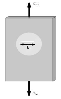
Figure 1: A material under the application of a uniform external stress $\sigma_{\infty}$ at its far edges in the presence of a crack of length $L$ that is cutting through the sample. The shaded region represents the typical area in which the potential energy density is changed relative to the uniform stress state.

In Fig. 1 we consider a material under the application of a uniform external stress $\sigma_{\infty}$ at its far edges. In addition, the material contains a single defect that is assumed here to be a crack of length $L$ that is cutting through the material. A crack is a region whose boundaries cannot support stress. In the absence of a crack the material is uniformly stressed with an associated potential energy density ${\cal E}_{p}$

$${\cal E}_{p}\sim\frac{\sigma^{2}_{\infty}}{E}\ ,$$ (1)

where $E$ is Young’s modulus and it is assumed that the material is linear elastic, resulting in a second-order energy density. The presence of a crack of length $L$ releases the stresses in an area of the order of $\sim L^{2}$ (shaded area in Fig. 1), resulting in a reduction $\Delta U_{p}$ in the potential energy per unit material width

$$\Delta U_{p}=-c_{p}\frac{\sigma^{2}_{\infty}L^{2}}{E}\ ,$$ (2)

where $c_{p}$ is a dimensionless factor. On the other hand, the very existence of the crack is associated with free material surface. Assuming that the energy cost per unit area of free surfaces is $\Gamma$, the generation of a crack of length $L$ results in an increase in the surface energy per unit width by an amount $\Delta U_{s}$,

$$\Delta U_{s}=\Gamma L\ .$$ (3)

The total energy change per unit width is

$$\Delta U=-c_{p}\frac{\sigma^{2}_{\infty}L^{2}}{E}+\Gamma L\ .$$ (4)

This equation tells us that for small values of $L$ the formation of a crack is costly ($\Delta U>0$) whereas longer cracks are energetically favorable ($\Delta U<0$). Actually, once a critical length is achieved the crack tends to increase indefinitely until the material completely fails. This non-equilibrium catastrophic crack propagation is at the essence of the failure of material. The two different regimes described above are separated by a Griffith critical length

$$L_{G}\sim\frac{E\Gamma}{\sigma_{\infty}}\ ,$$ (5)

which is shown to be a combination of material properties ($E$ and $\Gamma$) and external loading conditions ($\sigma_{\infty}$).

The thermodynamic argument predicts that crack propagation should always be catastrophic once initiated. In fact, although fast crack propagation is common, there are many situations in which the crack evolves quasi-statically. The point to stress is that whatever is the mode of crack growth, the argument exemplifies the multi-scale nature of the phenomenon; the potential energy released from the large scales dissipates in a very localized region near the crack tip where new crack surfaces are generated.

The technical discussion of crack propagation is classically done in the context of “linear elasticity fracture mechanics”. The state of deformation of the material is described by the displacement field ${\bf u(r)}$. This field consists of three translational degrees of freedom, where the local rotational degrees of freedom are neglected Cosserat . To develop a theory that is both translational and rotational invariant one defines the strain tensor $\epsilon_{ij}$, which is the symmetric part of the gradient of ${\bf u(r)}$

$$\epsilon_{ij}\equiv\frac{1}{2}\left(\partial_{i}u_{j}+\partial_{j}u_{i}\right)\ .$$ (6)

In a material that is homogeneous and isotropic, only the invariants of $\epsilon_{ij}$ can appear in the expression for the strain energy density ${\cal E}$. Restricting the analysis to a linear theory, i.e. to a quadratic strain energy density, we arrive at

$${\cal E}=\frac{1}{2}\left(2\mu~{}{\rm Tr}({\bm{\epsilon}}^{2})+\lambda~{}{\rm Tr}^{2}({\bm{\epsilon}})\right)\ ,$$ (7)

where the Lamé coefficients $\mu$ and $\lambda$ are material parameters that are related to the more common engineering constants $E$ (Young’s modulus) and $\nu$ (Poisson’s ratio). The stress tensor $\sigma_{ij}$ is related to the strain tensor via

$$\sigma_{ij}=\frac{\partial{\cal E}}{\partial\epsilon_{ij}}\ ,$$ (8)

which leads to a linear stress-strain relation

$$\sigma_{ij}=2\mu\epsilon_{ij}+\lambda\delta_{ij}\epsilon_{kk}\ .$$ (9)

The stress field is just the local force per unit area. Therefore, the Newton’s equations of motion for a unit volume of mass density $\rho$ are given by 86LL

$$\frac{\partial\sigma_{ij}}{\partial x_{j}}=\rho\frac{\partial^{2}u_{i}}{\partial t^{2}}\ .$$ (10)

Substituting Eq. (9) in the last set of equations we arrive at the Lamé equation

$$(\lambda+\mu){\bm{\nabla}}({\bm{\nabla}}\cdot{\bf u})+\mu\nabla^{2}{\bf u}=\rho\frac{\partial^{2}{\bf u}}{\partial t^{2}}\ .$$ (11)

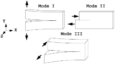
Figure 2: The typical symmetry modes of fracture, see text for more details.

Up to now the field equations for the medium were constructed disregarding the effects induced by the presence of a crack. At the level of linear elasticity fracture mechanics, the crack is introduced as boundary conditions. As was mentioned before, a crack is a region whose boundaries are free surfaces. Denote the unit normal to the crack surface at any point by $\hat{{\bf n}}$; the boundary conditions on the crack surface are

$$\sigma_{ij}n_{j}=0\ .$$ (12)

These boundary conditions introduce non-linearities into the problem even if the field equations themselves are linear. This is a major source of mathematical difficulties.

It is conventional to decompose the stress field under general loading conditions to three symmetry modes with respect to the fracture plane. These are illustrated in Fig. 2. In mode I the crack faces are displaced symmetrically in the normal direction relative to the fracture $xz$ plane, by tension. In mode II, the crack faces are displaced anti-symmetrically relative to the fracture $xz$ plane, in the $x$ direction, by shear. In these two modes of fracture the deformation is in-plane ($xy$). In mode III, the crack faces are displaced anti-symmetrically relative to the fracture plane, in the $z$ direction, by shear. This is an out-of-plane fracture mode.

The dissipation involved in the crack growth, quantified by the phenomenological material function $\Gamma$, is assumed to be highly localized near the crack front. Therefore, one is interested in the near crack front fields. Within linear elasticity theory these are actually singular. To see this consider first a quasi-static infinitesimal extension $\delta L$ of the crack. Denoting the stress field near the tip by $\sigma(r)$, the energy (per unit width) released from the linear elastic medium $\delta U$ is

$$\delta U\sim\int_{0}^{\delta L}\!\frac{\sigma^{2}(r)}{E}~{}r~{}dr\ .$$ (13)

This amount of energy is invested in creating new crack surfaces whose energy cost (per unit width) is $\Gamma\delta L$. Therefore, we must have

$$\sigma(r)\sim\frac{1}{\sqrt{r}}\ .$$ (14)

The inverse square-root singularity seen in Eq. (14) exists also in the fully dynamic case. In fact, by asymptotic expansion of the local stress tensor field near the crack front, it can be shown that the leading term is given by a sum of three contributions corresponding to the three modes of fracture 98Fre

$$\sigma_{ij}(r,\theta,t) =$$

$$K_{{}_{\rm I}}(t)\frac{\Sigma^{{}^{\rm I}}_{ij}(\theta,v)}{\sqrt{2\pi r}} + K_{{}_{\rm II}}(t)\frac{\Sigma^{{}^{\rm II}}_{ij}(\theta,v)}{\sqrt{2\pi r}}+K_{{}_{\rm III}}(t)\frac{\Sigma^{{}^{\rm III}}_{ij}(\theta,v)}{\sqrt{2\pi r}}\ ,$$

where $(r,\theta)$ are local polar coordinates system, $t$ is time, $v(t)$ is the local instantaneous front velocity, ${\bm{\Sigma}}^{(i)}(\theta,v)$ are universal and $K_{(i)}$ are the stress intensity factors. The stress intensity factors are non-universal functionals of the loading conditions, sample geometry and crack history. The predicted singular behavior is, of course, not physical and there must exist mechanisms to cut off this apparent singularity. Nevertheless, there are many physical situations for which the size of the region where linear elasticity breaks down is small compared to other relevant lengths. Therefore, the stress intensity factors are very important physical quantities and the singularity may be retained in many models. This singularity is a source of mathematical difficulties and physical riddles. The stress concentration quantified by the stress intensity factors shows that the material near a crack front experiences extreme conditions; the response to these conditions is far from being well-understood.

Up to now we have considered the case of a single straight crack in an otherwise linear homogeneous medium. A more realistic description of materials includes other sources of heterogeneity which exist in every material at some level. The effect of distributed sources of “disorder” calls for a statistical treatment. In developing such an approach one should understand the interplay between various fields and the material disorder, resulting in a complex spatio-temporal behavior. This complexity was studied extensively in the last decade, accumulating a wealth of relatively high precision experimental data and offering a real challenge for the theoretical physicist 99FM . In this paper we focus on one important aspect of the problem: the statistical physics of the morphology of quasi-static fracture surfaces. This subject has attracted a lot of interest recently and became a very active field of research 03Bou . The pioneering experimental work described in Ref. 84MPP drew attention to the fact that fracture surfaces are rough graphs in 2+1 (1+1) dimensions when the broken sample is three dimensional (two dimensional) and therefore might have anisotropic scaling properties. Suppose that the surface is described by its height $h(x,y)$ at position $(x,y)$ in a smooth reference plane. Consider now the probability density $P(\Delta h,\ell)$ that the height difference between two points in the reference plane separated by a length $\ell$ is within $d(\Delta h)$ of the height difference $\Delta h$. The anisotropic scaling properties of the surface manifest themselves through the following invariance under affine scale transformation

$$\lambda^{H}P(\lambda^{H}\Delta h,\lambda\ell)=P(\Delta h,\ell)\ ,$$ (16)

where $H$ is the roughness exponent. This is the starting point for the discussion of self affine properties of fracture surfaces. Later we will see that this definition is too limited and cannot capture the rich complexity exhibited by fracture surface morphology. The first part of this paper focuses on two dimensional fracture where the generated rupture lines are 1+1 dimensional graphs. In Sec. II we show that the statistical properties of rupture lines cannot be fully characterized by the scaling invariance of Eq. (16). In that case, the more complex structure of the probability distribution function leads to multiscaling in contrast with monoscaling implied by Eq. (16). We emphasize the properties of 1+1 dimensional disordered fracture needed to be explained by a proper theory. Sec. III offers a short critical review of existing theoretical approaches to the problem. We discuss the limitations of these approaches and explain why, in our opinion, they do not provide a satisfactory description of the underlying physics. In Sec. IV we describe a new theoretical model for the growth of a crack in a two dimensional medium in the presence of material disorder. We elaborate on the mathematical foundations of the model based on a recent development in which the method of iterated conformal maps was applied to the problem of elasticity in the presence of irregular crack geometries. We summarize the results of the model and show that they meet the basic requirements of Sec. II.

The second part of the paper discusses three dimensional fracture where the generated surfaces are 2+1 dimensional graphs. In Sec. V we show how the scaling properties of fracture surfaces can be rationalized by decomposing the height-height structure function into the irreducible representations of the $SO(2)$ symmetry group. This method offers a new way of understanding the anisotropic properties of fracture surfaces in the plane of fracture. We propose new experiments in which the rotational symmetry is not broken such that the scaling properties should be particularly simple. Sec. VI offers a summary and outlines for future research directions.

II Multiscaling in 1+1 Dimensional Fracture

In 1+1 dimensions one denotes the graph as $h(x)$, where $h$ is the height of the surface at point $x$ relative to a smooth reference line and considers the $n^{th}$ order structure function $S_{n}(\ell)$,

$$S_{n}(\ell)\equiv\langle|h(x+\ell)-h(x)|^{n}\rangle\ ,$$ (17)

where angular brackets denote an average over all $x$. These quantities are invariant under affine scale transformations if they are homogeneous functions of their arguments

$$S_{n}(\lambda\ell)\sim\lambda^{\zeta^{(n)}}S_{n}(\ell)\ .$$ (18)

If $\zeta^{(n)}$ is linearly related to $n$ the scaling properties of the graph are called “normal” and the graph is statistically self-affine. On the other hand, if $\zeta^{(n)}$ is a non-linear function of $n$, the structure functions are multiscaling (or anomalous) and the graph under consideration is called “multiaffine”. To our best knowledge, all the studies regarding fracture in 1+1 dimensions treated the rupture lines as normal graphs, implying that $\zeta^{(n)}=nH$ where $H$ is the roughness (Hurst) exponent. Note that $H>1/2$ indicates the existence of positive correlations in the process generating the surface which implies that an upward incremental deviation (relative to the smooth reference line) of the rupture line is more likely to be followed by an upward deviation than an downward one and vice versa 88Fed . This feature shows that the higher $H$ is, the smoother is the surface. Experimental analyses of rupture lines in quasi two-dimensional materials yielded a roughness exponent $H$ whose numerical value was close to $0.67$ 92PABT ; 93KHW ; 94EMHR ; 03SAN , suggesting some universality of the surface generating process. The proximity of this numerical value to the exact ratio $H=2/3$, characterizing the roughness of directed polymers in random media 95BS , has lead some authors to suggest that the two problems are in the same universality class 91HHRa ; 93KHW ; 95H-HZ ; 95BS . In this view, fracture is considered as a global minimization problem.

In a recent work 05BouP we have shown that the phenomenology is much richer and fracture lines are multiscaling. An example that provides us with information of sufficient accuracy to establish the multiscaling characteristics is rupture lines in paper. The data acquired by Santucci et al. 04SVC was obtained in experiments where centrally notched sheets of fax paper were fractured by standard tensile testing machine. Four resulting crack profiles $h(x)$ were digitized. Each digitization contained a few thousand points, where care was taken to insure that the smallest separation between points in $x$ is larger than the typical fiber width; this is important to avoid the artificial introduction of overhangs that destroy the graph property.

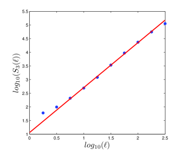
Figure 3: A log-log plot of $S_{3}(\ell)$ as a function of $\ell$. The linear fit corresponds to a typical scaling range of about $1.5$ orders of magnitude, with a slope of $\zeta^{(3)}\simeq 1.65$.

Denoting $\Delta h(\ell)\equiv h(x+\ell)-h(x)$ we analyzed the data by boxing $\ell$ in logarithmic boxes, accumulating the data between $10^{0}$ and $10^{0.25}$ (the smallest box) and between $10^{2.25}$ and $10^{2.5}$ (the largest box). The $m^{th}$ box was considered as representing data for $\ell=10^{m\times 0.25}$. On the basis of this boxing we constructed the probability distribution function (pdf) $P(\Delta h(\ell))$, which is just the probability distribution function defined in Eq. (16), by combining data from all the four samples. Samples that exhibit marked trends (probably due to the finite size of the sample), were detrended by subtracting the mean from each distribution. The computed pdf’s were then used to compute the moments (17), and these in turn, once presented as log-log plots, yield the scaling exponents $\zeta^{(n)}$. Such a typical log-log plot is shown in Fig. 3, exhibiting a typical scaling range of more than $1.5$ orders of magnitude. The resulting values of the scaling exponents $\zeta^{(n)}$ are shown in Fig. 4.

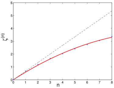
Figure 4: The spectrum $\zeta^{(n)}$ as a function of the moment order $n$ for rupture lines in paper. The function is fitted to the form $\zeta^{(n)}=nH-n^{2}\lambda$ and the parameters $H$ and $\lambda$ are given. The errors in the estimation of these parameters reflect both the variance between different samples and the fit quality. The linear plot $n\zeta^{(1)}$ is added to stress the non-linear nature of $\zeta^{(n)}$.

As a function of $n$ these numbers can be fitted to the quadratic function $\zeta^{(n)}=nH-n^{2}\lambda$ with $H=0.64\pm 0.03$ and $\lambda=0.026\pm 0.004$ (a linear plot $n\zeta^{(1)}$ is added for reference). The error bars quoted here reflect both the variance between different samples and the fit quality. The exponents were computed for $n\leq 8$ since for higher moments the discrete version of the integral

$$\int|\Delta h(\ell)|^{n}P(\Delta h(\ell))d\Delta h(\ell)$$ (19)

did not converge. On the other hand, the convergence of the $8^{th}$ order moment is demonstrated in Fig. 5.

Figure 5: An example of the convergence of the integral in Eq. (19) for $\ell=10^{2.25}$ and $n=8$.

The point to stress is that the scaling exponents $\zeta^{(n)}$ depend non-linearly on $n$; for the range of $n$ values for which the moments converge, the exponents can be fitted to a quadratic function. It is well known from other areas of nonlinear physics, and turbulence in particular 84AGHA ; 95Fri ; 05BP , that such phenomena of multiscaling are associated with pdf’s on different scales $\ell$ that cannot be collapsed by simple rescaling. In other words, in the absence of multiscaling, there exists a single scaling exponent $H$ with the help of which one can rescale the pdf’s according to

$$P(\Delta h(\ell))\sim\ell^{-H}f\left(\frac{\Delta h(\ell)}{\ell^{H}}\right)\ ,$$ (20)

where $f(\cdot)$ is a scaling function. In our case such rescaling does not result in data collapse. In Fig. 6 the natural logarithm of $P(\Delta h(\ell))\ell^{H}$ is plotted as a function of $\Delta h(\ell)/\ell^{H}$ for $H=0.64$. Indeed, the data does not collapse onto a single curve. The fatter tails of the probability distribution functions at smaller scales are typical to multiscaling situations, where the statistics of rare events plays an important role.

Figure 6: The natural logarithm of $P(\Delta h(\ell))\ell^{H}$ as a function of $\Delta h(\ell)/\ell^{H}$ for $H=0.64$. The legend gives the scale $\ell$ for each plot.

The multiscaling property of 1+1 dimensional fracture surfaces has an important implication; Since the problem of directed polymers in random media is monoscaling 91Hal , we conclude that the two problems are not in the same universality class. In fact none of the known kinetic growth model of statistical physics 95BS is consistent with the multiscaling spectrum discovered in 1+1 dimensional fracture. This might suggest that 1+1 dimensional fracture defines a distinct universality class in statistical physics, a proposition that must be checked against a much broader experimental data set. To conclude, the presence of multiscaling offers a stringent test for any theoretical model of 1+1 dimensional in-plane fracture.

III Traditional Theoretical Approaches

In the last fifteen years or so several statistical physics approaches were applied in this field. In this section we offer a short critical review of these approaches.

III.1 Lattice Models

The most studied model aiming at understanding the origin of self-affinity of fracture surfaces morphology, the value of the roughness exponent $H$ and its degree of universality is the quasi-static random fuse model book . This model consists of an array of identically conducting linear (Ohmic) resistors placed between two electrical bus bars with a fixed voltage difference. A threshold value $t_{j}$ taken from an uncorrelated distribution $p(t)$ is assigned to each resistor. At each step of the numerical simulation the Kirchhoff equations are solved and the current $i_{j}$ passing through each resistor is calculated. The system is advanced in time according to the extremal rule that states that the resistor with the largest ratio between current and threshold $max_{j}(i_{j}/t_{j})$ is irreversibly removed. The system is driven to its final state where the network of fuses stops conducting. The behavior of this model is controlled by the width of the threshold distribution $p(t)$ 91HHRb . For “very strong” disorder, i.e. for broad enough threshold distributions, the model behaves like a percolation problem, without any localized failure mode. For this regime, the disorder dominates the correlations which are induced by current enhancements due to removed resistors (the analog of stress concentration in the elastic problem). The cluster of broken bonds (removed resistors) shows no anisotropic scaling (formally, the roughness exponent $H$ is one in this case). For smaller disorders damage is distributed throughout the system, but at the “critical phase” of the dynamics of the model a localized failure mode sets in, resulting in a self-affine rupture line. At even smaller disorders, in the “weak” disorder regime, the system is “critical” from the early stages of the evolution in the sense that a large crack quickly nucleates and the dynamics is controlled by its propagation. The roughness exponent $H$ for the regimes where self-affine rupture lines are generated was measured to be $H\approx 0.7$ 91HHRa ; 00SRA .

Although the random fuse model is widely regarded “a paradigm for brittle fracture” 03HS , its capability to describe a real physical system that fails under external load is questionable; All the data on fracture surfaces morphology were obtained by in-plane fracture experiments, mainly in mode I, whereas the random fuse model is a discrete version of out-of-plane fracture (mode III), which is unstable experimentally unstable . While in-plane fracture modes entail the solution of the fully tensorial Lamé elasticity theory, out-of-plane fracture entails the solution of scalar elasticity theory, described by the Laplace equation. There is no a-priori reason to believe that the two problems are in the same universality class. Moreover, the random fuse model misrepresents another important feature of fracture experiments; when a material is externally loaded intrinsic defects can lead to the nucleation of a crack everywhere in the system. Since this process occurs in an uncontrolled way, it is an experimental convention to introduce a small crack in the sample prior to loading. Typically, the stress concentration near the tip of such a crack is so overwhelming that damage far from this region cannot develop significantly even in heterogenous materials. This is in contrast to the random fuse model, excluding situations of very narrow disorders, where damage is accumulated throughout the system prior to the critical phase of macroscopic failure in which the final rupture line develops. In spite of the inadequacy of the random fuse model to faithfully describe real physical systems, it might be useful to understand how positive correlations are built in the model, leading to $H>1/2$. Recently 03HS it was proposed that a correlated gradient percolation process is responsible for the value of the roughness exponent measured in this model. Here we do not give the argument in full detail, but focus on the main conceptual aspect of this proposition: correlations in the model are crucially dependent on the damage accumulated in the system before the critical phase of the formation of the final rupture line. In this view, the positive correlations observed in the final rupture line is a manifestation, via a coalescence process, of the long range positive correlations that are built in the system during the earlier stages of the dynamics. Therefore, this explanation rely heavily on the presence of a broad enough threshold distribution that is responsible for correlations in the precursory phase of the dynamics. On the other hand, other works 04NSZ ; 05RA support the view that correlations in the damage accumulated prior to the critical phase of macroscopic failure are negligible. If this view is valid then the origin of self-affine crack roughness in the random fuse model does not depend on whether there is “strong” or “weak” disorder since correlations are built in the system only at the final stage of macroscopic failure. We think that this view represents better the typical experimental situation where stress concentration near the pre-existing crack dominates the failure process. This view will be further developed below, see Sec. IV.

A second group of lattice models originated from the central force model book . In this model the lattice is connected by elastic springs that are freely rotating around the nodes. This model is much closer to real fracture since its continuum limit is the tensorial Lamé elasticity. Unfortunately, no systematic studies of the roughness exponent for this model were reported. A third group of lattice models is the random beam models. In these models the lattice is composed of elastic beams that are rigidly connected to the nodes. Here the bond bending elasticity is taken into account by considering the local rotational degrees of freedom at each node in addition to the translational ones that are described by the central force model. The roughness exponent in 1+1 dimensions for this model was found to be $H\approx 0.86$ 01SHH . Therefore, this model seems to be unrelated to the experimental findings. The origin of this discrepancy is probably the fact that Lamé elasticity provides an appropriate description of materials on a large enough length scale. To conclude, we propose that none of the lattice models found in the literature are capable of describing 1+1 dimensional in-plane fracture and to faithfully represent the experiments in the field.

III.2 Continuum Models

The basic issue arising in continuum models of crack propagation is how to predict where the crack goes under the action of a given stress field. One can use symmetry principles to derive an equation of motion for the crack tip. Adapting Eq. (LABEL:sigma) to two-dimensional quasi-static fracture, the stress tensor field attains the universal form

$$\sigma_{ij}(r,\theta)=\frac{K_{{}_{\rm I}}}{\sqrt{2\pi r}}\Sigma^{I}_{ij}(\theta)+\frac{K_{{}_{\rm II}}}{\sqrt{2\pi r}}\Sigma^{II}_{ij}(\theta)\ ,$$ (21)

where $I$ and $II$ denote the mode I (tensile) and mode II (shear) parts of the stress tensor field. As was explained above, the $r^{-1/2}$ singularity is not physical; nevertheless in many cases there exists a cut-off distance from the crack tip (a one-dimensional front), above which the stress field is dominated by the universal form. Therefore, the non-universal parts, the so-called stress intensity factors $K_{{}_{\rm I}}$ and $K_{{}_{\rm II}}$ are very important physical quantities.

In order to derive an equation of motion for the crack tip consider a curved crack in a two dimensional medium. The position of the crack tip is ${\bf r}^{tip}$ in some convenient coordinate system. Let us denote the unit tangent and the unit normal to the curved crack at its tip by $\hat{\bf t}$ and $\hat{\bf n}$ respectively and assume that the crack tip fields are characterized by the stress intensity factors $K_{{}_{\rm I}}$ and $K_{{}_{\rm II}}$. A discrete symmetry that the crack tip dynamics should remain invariant under its operation is $\hat{\bf n}\rightarrow-\hat{\bf n}$. Under this symmetry the relevant quantities in the problem transform as follows: (i) $K_{{}_{\rm I}}\rightarrow K_{{}_{\rm I}}$ (ii) $K_{{}_{\rm II}}\rightarrow-K_{{}_{\rm II}}$ (iii) $v\rightarrow v$. Now one can write down the most general first order differential equations that are invariant under this symmetry. The first equation is just the kinematic relation for the rate of crack growth

$$\frac{\partial{\bf r}^{tip}}{\partial t}=v(K_{{}_{\rm I}},K^{2}_{{}_{\rm II}})~{}\!\hat{\bf t}\ .$$ (22)

The second one describes the rate of crack tip rotation

$$\frac{\partial\hat{\bf t}}{\partial t}=-f(K_{{}_{\rm I}},K^{2}_{{}_{\rm II}},v)K_{{}_{\rm II}}\hat{\bf n}\ ,$$ (23)

where $f(K_{{}_{\rm I}},K^{2}_{{}_{\rm II}},v)$ is a positive material function. These equations were originally derived in 93HS and were shown to be consistent with various experimental observations in 03BHP ; 05BMP . To further simplify Eq. (23) we rewrite the local crack tip directions in terms of the angle $\theta$ that the unit tangent makes with the x-axis as

$$\hat{\bm{t}} = \cos{\theta}\hskip 2.84544pt\bf\hat{x}+\sin{\theta}\hskip 2.84544pt\bf\hat{y}$$

$$\hat{\bm{n}} = -\sin{\theta}\hskip 2.84544pt\bf\hat{x}+\cos{\theta}\hskip 2.84544pt\bf\hat{y}\ .$$ (24)

Using these expressions Eq. (23) can be written as

$$\frac{\partial\theta}{\partial t}=-f(K_{{}_{\rm I}},K^{2}_{{}_{\rm II}})K_{{}_{\rm II}}\ .$$ (25)

In order to use this equation, consider a long crack propagating quasi-statically in a two dimensional medium under mode I conditions. If the medium were homogenous, we would have $K_{{}_{\rm II}}\{h(x)\}=0$, and according to Eq. (25) the crack would extend along a straight path. Real material possess however some inhomogeneities which induces fluctuations $h(x)$ in the crack path. The global symmetry is broken locally, leading to $K_{{}_{\rm II}}\{h(x)\}\neq 0$. $K_{{}_{\rm II}}\{h(x)\}$ is a functional of the fluctuations $h(x)$, typically including a long-range contribution, reflecting the long-range nature of the elastic interactions and a local contribution. If we restrict ourselves to small fluctuations $h(x)$ we obtain $\theta\approx\partial_{x}h$. Furthermore, by considering steady state propagation such that $\partial_{t}\rightarrow v\partial_{x}$ and representing the effect of material disorder by a noise term $\vartheta(x)$, we arrive at the following Langevin type equation

$$\frac{v}{f}~{}\partial_{xx}h(x)=-K^{(1)}_{{}_{\rm II}}\{h(x)\}-\vartheta(x)\ ,$$ (26)

where the superscript $(1)$ denotes the fact the $K_{{}_{\rm II}}\{h(x)\}$ is considered to first order in the small fluctuation $h(x)$ and the disorder is modeled as uncorrelated noise

$$\langle\vartheta(x)\vartheta(x^{\prime})\rangle\sim\delta(x-x^{\prime})\ .$$ (27)

The mode II stress intensity factor, $K_{{}_{\rm II}}\{h(x)\}$, was calculated in first order perturbation theory in 80CR , yielding

$$K^{(1)}_{{}_{\rm II}}\{h(x)\}=\!\frac{1}{2}K^{(0)}_{{}_{\rm I}}\partial_{x}h+\sqrt{\frac{2}{\pi}}\int_{-\infty}^{x}\!\!\frac{\partial_{x^{\prime}}(h(x^{\prime})\sigma^{(0)}_{xx}(x^{\prime}))}{\sqrt{-x^{\prime}}}dx^{\prime}\!\!\ ,$$ (28)

where the superscript $(0)$ denotes quantity of the unperturbed solution. By considering a configuration in which $\sigma^{(0)}_{xx}(x^{\prime})$ is practically constant, a scaling analysis of Eq. (26) results in a logarithmic roughness of the rupture line. A similar treatment as the one presented here was developed in 97REF where higher order terms were shown to be irrelevant in the renormalization group sense. It is concluded that this approach does not produce any non-trivial roughness exponent. The reason for this failure is, in our opinion, the fact that the crack growth takes place at the tip which is controlled completely by the stress intensity factor $K_{{}_{\rm II}}$. We will show that there are observations that motivate the view that the crack growth is a discrete process taking place via the nucleation of damage at a finite distance $R$ ahead of the crack tip. This length $R$ characterizes the scale of “spikiness” of the crack path; thus, when the growth step takes place at a distance $R$ ahead of the crack tip the irregularities of the crack path (“spikiness”) change the structure of the stress field and a different long range quantity controls the growth process. Moreover, the irregularities of the crack path are difficult to handle using perturbative approaches. The effect of this finite length scale on the crack growth is further discussed in the next section. We conclude this section by noting that the origin of the long range positive correlations in 1+1 dimensional fracture and its multiscaling nature are not yet explained by the existing models.

IV A Model

In this section we review a recently introduced statistical model of crack surfaces morphology in 1+1 dimensional fracture which takes into account the insights gained from both experiments and previous theoretical approaches. It is common to divide the failure of materials into two categories: ductile and brittle. In brittle fracture materials break when subjected to large enough stresses without large plastic deformations taking place. In ductile fracture, on the other hand, materials undergo significant plastic flow before experiencing any local failure. In this case a crack evolves by the nucleation, growth and coalescence of voids. A recent experiment 03C motivated the view that quasi-static brittle fracture occurs, similarly to ductile fracture, by the nucleation of damage ahead of the crack tip. It is not clear yet if this process necessarily involves plastic deformations. The length scale of damage nucleation $R$ in traditional “brittle” and “ductile” materials is completely different. Nevertheless, we suggest that this behavior is generic irrespective of whether the physics behind this length scale is related to plastic deformation or to existing material disorder.

Therefore, a statistical theory of crack surfaces morphology in 1+1 dimensions should include the following components: (i) the exact solution of the elasticity problem in the presence of irregular crack geometries (ii) a growth law in which the evolution of the crack is controlled by the nucleation of voids at a finite distance $R$ ahead of the crack tip (iii) an appropriate description of the effect of material disorder.

IV.1 The elasticity problem in the presence of irregular crack geometries

In this section we review a non-perturbative approach to the calculation of the stress field in two space dimensions for an arbitrarily shaped crack, based on conformal mapping 04BMPa . We start with the quasi-static version of Eq. (10), obtained by dropping the inertial term on the right hand side

$$\frac{\partial\sigma_{ij}}{\partial x_{j}}=0.$$ (29)

For in-plane modes of fractures in two dimensions one introduces the Airy stress potential $U(x,y)$ such that

$$\sigma_{xx}=\frac{\partial^{2}U}{\partial y^{2}}\ ;\sigma_{xy}=-\frac{\partial^{2}U}{\partial x\partial y}\ ;\sigma_{yy}=\frac{\partial^{2}U}{\partial x^{2}}\ .$$ (30)

Thus the set of Eq. (29), after simple manipulations, translate to a bi-Laplace equation for the Airy stress potential $U(x,y)$ 86LL

$$\nabla^{2}\nabla^{2}U(x,y)=0\ ,$$ (31)

with the prescribed boundary conditions on the crack and on the external boundaries of the material. At this point we choose to focus on the case of uniform remote loadings and traction-free crack boundaries. This choice, although not the most general, is of great interest and will serve to elucidate our method. Other solutions may be obtained by superposition. Thus, the boundary conditions at infinity, for the two in-plane symmetry modes of fracture, are presented as

$$\!\!\!\!\!\!\!\!\sigma_{xx}(\infty)=0\ ;\sigma_{yy}(\infty)=\sigma_{\infty}\ ;\sigma_{xy}(\infty)=0\quad\text{Mode I}$$ (32)

$$\!\!\!\!\!\!\!\!\sigma_{xx}(\infty)=0\ ;\sigma_{yy}(\infty)=0\ ;\sigma_{xy}(\infty)=\sigma_{\infty}\quad\text{Mode II}\ .$$

(33)

In addition, the free boundary conditions on the crack are expressed as

$$\sigma_{xn}(s)=\sigma_{yn}(s)=0\ ,$$ (34)

where $s$ is the arc-length parametrization of the crack boundary and the subscript $n$ denotes the outward normal direction $\hat{{\bf n}}$.

The solution of the bi-Laplace equation can be written in terms of two analytic functions $\phi(z)$ and $\eta(z)$ as

$$U(x,y)=\Re[\bar{z}\varphi(z)+\eta(z)]\ .$$ (35)

In terms of these two analytic functions, using Eq. (30), the stress components are given by

$$\sigma_{yy}(x,y) = \Re[2\varphi^{\prime}(z)+\bar{z}\varphi^{\prime\prime}(z)+\eta^{\prime\prime}(z)]$$

$$\sigma_{xx}(x,y) = \Re[2\varphi^{\prime}(z)-\bar{z}\varphi^{\prime\prime}(z)-\eta^{\prime\prime}(z)]$$

$$\sigma_{xy}(x,y) = \Im[\bar{z}\varphi^{\prime\prime}(z)+\eta^{\prime\prime}(z)].$$ (36)

In order to compute the full stress field one should first formulate the boundary conditions in terms of the analytic functions $\varphi(z)$ and $\eta(z)$ and to remove the gauge freedom in Eq. (35). The boundary conditions Eq. (34), using Eq. (30), can be rewritten as 53Mus

$$\partial_{s}\left[\frac{\partial U}{\partial x}+i\frac{\partial U}{\partial y}\right]=0\ .$$ (37)

Note that we do not have enough boundary conditions to determine $U(x,y)$ uniquely. In fact we can allow in Eq. (35) arbitrary transformations of the form

$$\varphi \rightarrow \varphi+iCz+\gamma$$

$$\psi \rightarrow \psi+\tilde{\gamma}\ ,\quad\psi\equiv\eta^{\prime}$$ (38)

where $C$ is a real constant and $\gamma$ and $\tilde{\gamma}$ are complex constants. This provides five degrees of freedom in the definition of the Airy potential. Two of these freedoms are removed by choosing the gauge in Eq. (37) according to

$$\frac{\partial U}{\partial x}+i\frac{\partial U}{\partial y}=0\ ,\quad\text{on the boundary}\ .$$ (39)

It is important to stress that whatever the choice of the five freedoms, the stress tensor is unaffected; see 53Mus for an exhaustive discussion of this point. Computing Eq. (39) in terms of Eq. (35) we arrive at the boundary condition

$$\varphi(z)+z\overline{\varphi^{\prime}(z)}+\overline{\psi(z)}=0\ .$$ (40)

To proceed we represent $\varphi(z)$ and $\psi(z)$ in Laurent expansion form:

$$\varphi(z) = \varphi_{1}z+\varphi_{0}+\varphi_{-1}/z+\varphi_{-2}/z^{2}+\cdots\ ,$$

$$\psi(z) = \psi_{1}z+\psi_{0}+\psi_{-1}/z+\psi_{-2}/z^{2}+\cdots\ .$$ (41)

This form is in agreement with the boundary conditions at infinity that disallow higher order terms in $z$. One freedom is now used to choose $\varphi_{1}$ to be real and two more freedoms will allow us later on to fix $\varphi_{0}$. Then, using the boundary conditions (32) and (33), we find

$$\varphi_{1} = \frac{\sigma_{\infty}}{4}\ ;\quad\psi_{1}=\frac{\sigma_{\infty}}{2}\quad\text{ Mode I}\ ,$$

$$\varphi_{1} = 0\ ;\quad\quad\psi_{1}=i\sigma_{\infty}\quad\text{ Mode II}\ .$$ (42)

As said above, the direct determination of the stress tensor for a given arbitrary shaped crack is difficult. To overcome the difficulty we perform an intermediate step of determining the conformal map from the exterior of the unit circle to the exterior of our given crack. Before our work the best available approach for such a task was the Schwartz-Cristoffel transformation. We have presented an alternative new approach for finding the wanted conformal transformation, given in terms of a functional iteration of fundamental conformal maps. The use of iterated conformal maps was pioneered by Hastings and Levitov 98HL ; it was subsequently turned into a powerful tool for the study of fractal and fracture growth patterns 99DHOPSS ; 00DFHP ; 00DLP ; 01BJLMP ; 01BDLP ; 02BLP ; 05MPST . In the next subsection we describe how, given a crack shape, to construct a conformal map from the complex $\omega$-plane to the physical $z$-plane such that the conformal map $z=\Phi(\omega)$ maps the exterior of the unit circle in the $\omega$-plane to the exterior of the crack in the physical $z$-plane, after $n$ directed growth steps. We draw the reader’s attention to the fact that this method is more general than its application in this paper 05MPST , and in fact we offer it as a superior method to the Schwartz-Cristoffel transformation, with hitherto undetermined potential applications in a variety of two-dimensional contexts.

Figure 7: Example of how to construct the conformal mapping along a line, see text for details.

IV.1.1 The conformal mapping

The essential building block in the present application, as in all the applications of the method of iterated conformal maps is the fundamental map $\phi_{\lambda,\theta}$ that maps the exterior circle onto the unit circle with a semi-circular bump of linear size $\sqrt{\lambda}$ which is centered at the point $e^{i\theta}$. This map reads 98HL :

$$\phi_{0,\lambda}(w)=\sqrt{w}\left\{\frac{(1+\lambda)}{2w}(1+w)\right.$$ (43)

$$\left.\times\left[1+w+w\left(1+\frac{1}{w^{2}}-\frac{2}{w}\frac{1-\lambda}{1+\lambda}\right)^{1/2}\right]-1\right\}^{1/2}$$

$$\phi_{\theta,\lambda}(w)=e^{i\theta}\phi_{0,\lambda}(e^{-i\theta}w)\,.$$ (44)

The inverse mapping $\phi^{-1}_{\theta=0,\lambda}$ is of the form

$$\phi^{-1}_{0,\lambda}=\frac{\lambda z-\sqrt{1+\lambda}(z^{2}-1)}{1-(1+\lambda)z^{2}}z\ .$$ (45)

By composing this map with itself $n$ times with a judicious choice of series $\{\theta_{k}\}_{k=1}^{n}$ and $\{\lambda_{k}\}_{n=1}^{n}$ we will construct $\Phi^{(n)}(\omega)$ that will map the exterior of the circle to the exterior of an arbitrary simply connected shape. To understand how to choose the two series $\{\theta_{k}\}_{k=1}^{n}$ and $\{\lambda_{k}\}_{n=1}^{n}$ consider Fig. 7 and define the inverse map $\omega=\chi^{(n)}(z)$. Assume now that we already have $\Phi^{(n-1)}(\omega)$ and therefore also its analytic inverse $\chi^{(n-1)}(z)$ after $n-1$ growth steps and we want to perform the next iteration. To construct $\Phi^{(n)}(\omega)$ we advance our mapping in the direction of a point $\tilde{z}$ in the $z$-plane by adding a bump in the direction of $\tilde{w}=\chi^{(n-1)}(\tilde{z})$ in the $w$-plane. The map $\Phi^{(n)}(\omega)$ is obtained as follows:

$$\Phi^{(n)}(\omega)=\Phi^{(n-1)}(\phi_{\theta_{n},\lambda_{n}}(\omega))\ .$$ (46)

The value of $\theta_{n}$ is determined by

$$\theta_{n}=\arg[\chi^{(n-1)}(\tilde{z})]$$ (47)

The magnitude of the bump $\lambda_{n}$ is determined by requiring fixed size bumps in the $z$-plane. This means that

$$\lambda_{n}=\frac{\lambda_{0}}{|{\Phi^{(n-1)}}^{\prime}(e^{i\theta_{n}})|^{2}}.$$ (48)

We note here that it is not necessary in principle to have fixed size bumps in the physical domain. In fact, adaptive size bumps could lead to improvements in the precision and performance of our scheme. We consider here the fixed size scheme for the sake of simplicity and we will show that the accuracy obtained is sufficient for our purposes. Iterating the scheme described above we end up with a conformal map that is written in terms of an iteration over the fundamental maps (43):

$$\Phi^{(n)}(w)=\phi_{\theta_{1},\lambda_{1}}\circ\ldots\circ\phi_{\theta_{n},\lambda_{n}}(w)\ .$$ (49)

For the sake of newcomers to the art of iterated conformal maps we stress that this iterative structure is abnormal, in the sense that the order of iterates in inverted with respect to standard dynamical systems. On the other hand the inverse mapping follows a standard iterative scheme

$$\chi^{(n)}(z)=\phi^{-1}_{\theta_{n},\lambda_{n}}\circ\ldots\circ\phi^{-1}_{\theta_{1},\lambda_{1}}(z)\ .$$ (50)

The algorithm is then described as follows; first we divide the curve into segments separated by points $\{z_{i}\}$. The spatial extent of each segment is taken to be approximately $\sqrt{\lambda_{0}}$, in order to match the size of the bumps in the $z$-plane. Without loss of generality we can take one of these points to be at the center of coordinates and to be our starting point. From the starting point we now advance along the shape by mapping the next point $z_{i}$ on the curve according to the scheme described above.

IV.1.2 Solution in terms of conformal mappings

The conformal map $\Phi^{(n)}(\omega)$ is constructed in $n$ iterative steps. For the discussion below we do not need the $n$ superscript and will denote simply $\Phi(\omega)\equiv{\Phi}^{(n)}(\omega)$. This map is univalent 99DHOPSS , having the Laurent expansion form

$$\Phi(\omega)=F_{1}\omega+F_{0}+F_{-1}/\omega+F_{-2}/\omega^{2}+\cdots\ .$$ (51)

Any position $z$ in the physical domain is mapped by $\chi(z)\equiv{\Phi}^{-1}(z)$ onto a position $\omega$ in the mathematical domain. This transformation does not immediately provide the solution as the bi-Laplace equation, in contrast to the Laplace equation, is not conformally invariant. Nevertheless, the conformal mapping method can be extended to non-Laplacian problems. We begin by writing our unknown functions $\varphi(z)$ and $\psi(z)$ in terms of the conformal map

$$\varphi(z)\equiv\tilde{\varphi}\left(\chi(z)\right)\ ,\quad\psi(z)\equiv\tilde{\psi}\left(\chi(z)\right)\ .$$ (52)

Using the Laurent form of the conformal map, Eq. (51), the linear term as $\omega\to\infty$ is determined by Eqs. (52). We therefore write

$$\tilde{\varphi}(\omega) = \varphi_{1}F_{1}\omega+\tilde{\varphi}_{-1}/\omega+\tilde{\varphi}_{-2}/\omega^{2}+\dots\ ,$$

$$\tilde{\psi}(\omega) = \psi_{1}F_{1}\omega+\tilde{\psi}_{0}+\tilde{\psi}_{-1}/\omega+\tilde{\psi}_{-2}/\omega^{2}+\dots\ ,$$ (53)

where we used the last two freedoms to choose $\varphi_{0}=-F_{0}\varphi_{0}$ such that $\tilde{\varphi}_{0}=0$. The boundary condition (40) is now read for the unit circle in the $\omega$-plane. Denoting $\epsilon\equiv e^{i\theta}$ and

$$u(\epsilon)\equiv\sum_{k=1}^{\infty}\tilde{\varphi}_{-k}/\epsilon^{k}\ ,\quad v(\epsilon)\equiv\sum_{k=0}^{\infty}\tilde{\psi}_{-k}/\epsilon^{k}\ ,$$ (54)

we write

$$u(\epsilon)+\frac{\Phi(\epsilon)}{\overline{\Phi^{{}^{\prime}}(\epsilon)}}\overline{u^{\prime}(\epsilon)}+\overline{v(\epsilon)}=f(\epsilon)\ .$$ (55)

The function $f(\epsilon)$ is a known function that contains all the coefficients that were determined so far:

$$f(\epsilon)=-\varphi_{1}F_{1}\epsilon-\frac{\Phi(\epsilon)}{\overline{\Phi^{{}^{\prime}}(\epsilon)}}\varphi_{1}F_{1}-\frac{\overline{\psi_{1}}F_{1}}{\epsilon}\ .$$ (56)

To solve the problem we need to compute the coefficients $\tilde{\varphi}_{n}$ and $\tilde{\psi}_{n}$. To this aim we first write 02BLP

$$\frac{\Phi(\epsilon)}{\overline{\Phi^{{}^{\prime}}(\epsilon)}}=\sum_{-\infty}^{\infty}b_{i}\epsilon^{i}.$$ (57)

The function $f(\epsilon)$ has also an expansion of the form

$$f(\epsilon)=\sum_{-\infty}^{\infty}f_{i}\epsilon^{i}\ .$$ (58)

In the discussion below we assume that the coefficients $b_{i}$ and $f_{i}$ are known. In order to compute these coefficients we need to Fourier transform the function $\Phi(\epsilon)/\overline{\Phi^{{}^{\prime}}(\epsilon)}$. This is the most expensive step in our solution. One needs to carefully evaluate the Fourier integrals between the branch cuts. Using the last two equations together with Eqs. (54) and (55) we obtain

$$\tilde{\varphi}_{-m} - \sum_{k=1}^{\infty}k~{}b_{-m-k-1}\tilde{\varphi}^{*}_{-k}=f_{-m}\ ,\quad m=1,2\cdots\ ,$$ (59)

$$\tilde{\psi}^{*}_{-m} - \sum_{k=1}^{\infty}k~{}b_{m-k-1}\tilde{\varphi}^{*}_{-k}=f_{m}\ .\quad m=0,1,2\cdots\$$ (60)

These sets of linear equations are well posed. The coefficients $\tilde{\varphi}_{-m}$ can be calculated from equation (59) alone, and then they can be used to determine the coefficients $\tilde{\psi}_{-m}$. This is in fact a proof that Eq. (55) determines the functions $u(\epsilon)$ and $v(\epsilon)$ together. This fact had been proven with some generality in 53Mus .

The calculation of the Laurent expansion form of $\tilde{\varphi}(\omega)$ and $\tilde{\psi}(\omega)$ provides the solution of the problem in the $\omega$-plane. Still, one should express the derivatives of $\varphi(z)$ and $\eta(z)$ in terms of $\tilde{\varphi}(\omega)$ and $\tilde{\psi}(\omega)$ and the inverse map $\chi(z)$ to obtain the solution in the physical $z$-plane. This is straight forward and yields

$$\varphi^{\prime}(z) = \tilde{\varphi}^{\prime}[\chi(z)]~{}\chi^{\prime}(z)$$

$$\varphi^{\prime\prime}(z) = \tilde{\varphi}^{\prime\prime}[\chi(z)]~{}[\chi^{\prime}(z)]^{2}+\tilde{\varphi}^{\prime}[\chi(z)]~{}\chi^{\prime\prime}(z)$$

$$\eta^{\prime\prime}(z) = \psi^{\prime}(z)=\tilde{\psi}^{\prime}[\chi(z)]~{}\chi^{\prime}(z).$$ (61)

Upon substituting these relations into Eq. (36) one can calculate the full stress field for an arbitrarily shaped crack. The expression of the stress field in terms of the inverse conformal mapping is known for quite a long time although it is very limited as the conformal mapping and its inverse is rarely at hand. The central step of progress here is the conjunction of the novel functional iterative scheme for obtaining the inverse conformal mapping with the known result that expresses the stress field in terms of this inverse mapping. This method was shown in 04BMPa to reproduce results for known regular crack geometries.

IV.2 A Crack Growth Law

After developing the mathematics needed for the calculation of the linear elastic stress field for irregular crack geometries, we turn now to a description of the crack growth law and the effect of disorder. As was explained above, a crucial aspect of the crack growth process is the finite length scale $R$ in which damage nucleates. A simple model 04BMPb ; 05ABKMP for $R$ can be developed by assuming the near crack tip zone to be properly described by the Huber-von Mises plasticity theory 90Lub . This theory focuses on the deviatoric stress $s_{ij}\equiv\sigma_{ij}-\frac{1}{3}{\rm Tr}({\bm{\sigma}})\delta_{ij}$ and on its invariants. The second invariant, $J_{2}\equiv\frac{1}{2}s_{ij}s_{ij}$, corresponds to the distortional energy. The material yields as the distortional energy exceeds a material-dependent threshold $\sigma_{{}_{\rm Y}}^{2}$. The fact that we treat this threshold as a constant, independent of the state of deformation and its history, implies that we specialize for “perfect” plasticity. In two-dimensions this yield condition reads 90Lub

$$J_{2}=\frac{\sigma^{2}_{1}-\sigma_{1}\sigma_{2}+\sigma^{2}_{2}}{3}=\sigma^{2}_{{}_{\rm Y}}\ .$$ (62)

Here $\sigma_{1\!,2}$ are the principal stresses given by

$$\sigma_{1\!,2}=\frac{\sigma_{yy}+\sigma_{xx}}{2}\pm\sqrt{\frac{(\sigma_{yy}-\sigma_{xx})^{2}}{4}+\sigma_{xy}^{2}}\ .$$ (63)

In the purely linear-elastic solution the crack tip region is where high stresses are concentrated. Perfect plasticity implies on the one hand that the tip is blunted and on the other hand that inside the plastic zone the Huber-von Mises criterion (62) is satisfied. The outer boundary of the plastic zone will be called below the “yield curve”, and in polar coordinates around the crack tip will be denoted ${\cal R}(\theta)$. Below we will compute the outer stress field exactly as was explained in the previous section. Using this field we can find the yield curve ${\cal R}(\theta)$. Such a typical curves are shown in the insets of Figs. 8 and 10.

Whatever is the actual shape of the blunted tip its boundary cannot support stress. Together with Eq. (62) this implies that on the crack interface

$$\sigma_{1}=\sqrt{3}~{}\sigma_{{}_{\rm Y}}\!,~{}~{}~{}~{}~{}~{}\sigma_{2}=0.$$ (64)

The typical scale $R$ follows from the physics of the nucleation process. It is physically plausible that void formation is more susceptible to hydrostatic tension than to distortional stresses. We assume that void nucleation occurs where the hydrostatic tension $P$, $P\equiv\frac{1}{2}$Tr${\bm{\sigma}}$, exceeds some threshold value $P_{c}$. The calculated the hydrostatic tension $P$ along the yield curve is found to be significantly higher than its value on the crack surface $P=\frac{\sqrt{3}}{2}\sigma_{{}_{\rm Y}}$ (cf. Eq. (64)). On the other hand the linear-elastic solution implies a monotonically decreasing P outside the yield curve. We thus expect P to attain its maximum value between the blunted crack tip and the yield curve. This conclusion is fully supported by finite elements method calculations, cf. 77McM . As the detailed elastic-plastic crack tip fields are not computed here, we use the outer elastic solution on the yield curve to determine the void nucleation position. We expect that this approximation should not affect the roughening exponents on large scales. The distance from the crack tip where $P$ attains its maximal value is of the order of the size of the plastic zone.

In this model the nucleation occurs when P exceeds a threshold $P_{c}$. The void will thus appear at a typical distance $R$. A very clear demonstration of the appearance of the void near the boundary of the plastic zone is seen in the molecular dynamics simulations of 99Falk . Note that $R$ is not a newly found length scale; it is the well known scale of the plastic zone 68Rice . Its identification with a length scale that is related to the scaling behavior of fracture surfaces is however new. This stems from the proposition that positive correlations appear only between the positions of nucleated voids. Below $R$ one enters the regime of plastic processes whose theory is far from being settled. We should also comment that it is possible that positive correlations appear even below the scale of the plastic zone since experiments indicate that several voids nucleate within the plastic zone 99BP ; 03Cil . Finally, we note that the assumption of perfect plasticity, i.e. that $\sigma_{{}_{\rm Y}}$ is independent of the state of deformation and its history, is not true for real materials; usually $\sigma_{{}_{\rm Y}}$ is not sharply defined; it can increase with plastic deformations 90Lub . This phenomenon, known as “work-hardening” or “strain-hardening” is not taken into account in this simple model, with the hope to be irrelevant for the crack morphology on large scales.

Naturally, the precise location of the nucleating void will experience a high degree of stochasticity due to material disorder. A basic assumption behind our treatment of this stochasticity is that the material disorder occurs on scales smaller than $R$, allowing us to introduce a probability distribution function that is a function of the hydrostatic tension on the yield curve. Since we do not know from first principles the probability distribution for void formation, we consider in our model below two possible distribution functions. In all cases nucleation cannot occur if $P<P_{c}$. For $P>P_{c}$ the void occurs with probability

$$P \propto P-P_{c}\ ,$$ (65)

$$P \propto \exp[\alpha(P-P_{c})]-1\ .$$ (66)

In the exponential case we considered two different values of $\alpha$. In Fig. 8 we show three such pdf’s as they appear for a perfectly straight crack. We note that these distributions are symmetric about the forward direction. Nevertheless they have sufficient width to allow deviations from forward growth. These deviations will be responsible later for the roughening of the crack. For comparison examine also the pdf’s for a general crack which are shown in Fig. 10. There the symmetry is lost: correlation to previous steps create a preference for the upward direction.

Figure 8: Panel (i): the tip of a straight crack and the yield curve in front of it.
Panel (ii): three probability distribution functions calculated for the configuration in (i). The abscissa is $\theta$, the angle measured from the crack tip as seen in panel (i). The ordinate is the normalized probability (per unit $\theta$) to grow in the $\theta$ direction. The distributions are symmetric and wide enough to allow deviations from the forward direction. For all the curves $\frac{\sigma_{{}_{\rm Y}}}{\sigma^{\infty}}=6$. For curve (a) $\mathrm{p}(\theta)\propto\exp[(P-P_{c})]-1$ and $\frac{P_{c}}{\sigma^{\infty}}=8$, for curve (b) $\mathrm{p}(\theta)\propto\exp[0.2(P-P_{c})]-1$ and $\frac{P_{c}}{\sigma^{\infty}}=6$ and for curve (c) $\mathrm{p}(\theta)\propto P-P_{c}$ and $\frac{P_{c}}{\sigma^{\infty}}=6$.

Each growth step in our model is composed of two events. Firstly the material yields near the crack tip, creating a plastic zone with a void growing somewhere at the zone boundary. Secondly the crack tip and the void coalesce. We note that there is a separation of time scales between these two events. The first is slow enough to be governed by a quasi-static stress field. The second event occurs on a shorter time scale. It is clear that we forsake in the model any detailed description of the geometry on scales smaller than $R$. Any relevant scaling exponent that will be found in this model will refer to roughening on length scales larger than $R$. Therefore, the physical process in which the crack coalesces with the multiple voids ahead of it is substituted by a single void coalescence with the crack.

IV.3 Results

Calculating the stress field around the crack, according to the method of iterated conformal maps, we can readily find the yield curve and the physical region in its vicinity where a void can be nucleated. Choosing with any one of the probability distributions described above, we use this site as a pointer that directs the crack tip. We then use the method of iterated conformal mappings to make a growth step to coalesce the tip with the void. Naturally the step sizes are of the order of $R$. We reiterate that this model forsakes the details of the void structure and all the length scales below $R$. Since we are making linear steps below $R$, we anticipate having an artificial scaling exponent $H=1$ for scales smaller than $R$. This is clearly acceptable as long as we are mainly interested in the scaling properties on scales larger than $R$.

Figure 9: Two typical cracks generated with our model. Note the huge difference in scales of the abscissa and ordinate (the cracks are globally flat) and that the lower crack had been translated by -300. The upper crack exhibits two decades of self-affine scaling with a Hurst exponent $0.64$. The lower crack has smaller standard deviation and therefore a shorter scaling range. Nevertheless it appears that in its shorter scaling range it exhibits an exponent that is very close to the upper crack.

In Fig. 9 we present two typical cracks that were grown using this method. Both cracks were initiated from a straight crack of length 10000, representing the experimental paradigm of introducing a notch before loading the sample. The upper crack was grown using the broader exponential pdf of Fig. 10 curve (b). The lower crack was grown with the narrower pdf of Fig. 10 curve (a). Clearly, the upper crack exhibits stronger height fluctuations, as can be expected from the wider pdf and the choice of parameters. For the lower crack forward growth is much more preferred. In the upper crack the positive correlations between successive void nucleation and coalescence events can be seen even with the naked eye. This is precisely the property that we were after. A neat way to see this tendency is in the pdf’s as they are computed on the yields crack for a typical, rather than straight, crack. In Fig. 10 we show these pdf’s for the crack whose yield curve is shown in the upper panel. We see that now the symmetry of the pdf’s is lost, and positive values of $\theta$ are preferred. This is the source of positive correlations that eventually gives rise to a non-trivial roughening exponent.

Figure 10: Panel (i): the tip of a “rough” crack and the yield curve in front of it. Panel (ii): three probability distribution functions calculated for the configuration in panel (i). The abscissa is $\theta$, the angle measured from the crack tip as seen in panel (i). The ordinate is the normalized probability (per unit $\theta$) to grow in the $\theta$ direction. The pdf’s are those used in Fig. 8, using the same parameters. Note the upward preference in all the pdf’s due to the broken symmetry.

This is born out by the measurements of the scaling properties of the fracture lines morphology that we discuss next.

We first restrict ourselves to a monoscaling analysis. Due to the significant computational cost of the iterated conformal maps technique the numerical investigation of the growth model had a limited number of realizations of a few hundreds growth steps. As a result of the relative paucity of data, the structure functions defined in Eq. (17) would not converge well enough to provide reliable exponents. Comparing the various available methods for estimating roughness exponents 95SVR we decided to select the max-min method, which seems to give reliable results in our case. Therefore, one defines $S(\ell)$ according to

$$S(\ell)\equiv\left<Max\left\{y(\tilde{x})\right\}_{x<\tilde{x}<x+\ell}-Min\left\{y(\tilde{x})\right\}_{x<\tilde{x}<x+\ell}\right>_{x}\ .$$ (67)

For self-affine graphs the Hurst exponent $H$, as was explained in the introduction, is obtained via the scaling relation

$$S(\ell)\sim\ell^{H}\ .$$ (68)

In Fig. 11 we present a typical log-log plot of $S(\ell)$ vs. $\ell$, in this case for the two cracks in Fig. 9 with power-law fits of $H=0.64$ and $H=0.68$ respectively. Indeed, as anticipated from the visual observation of Fig. 9 the exponent is higher than 0.5.

Figure 11: Calculation of the roughening exponent $H$. The slopes of the dotted lines are $0.64$ for the upper plot (curve a) and 0.68 for the lower (curve b). Note that the initial scaling with slope $1$ is relevant for length scales smaller than $R$. This scaling is an artifact, resulting from our algorithm that connects the crack tip to a void by a straight line.

It turned out that all the cracks grown by our algorithm gave rise to scaling plots in which a scaling range with $H=0.66\pm 0.03$ is clearly seen. When the pdf allowed for a sizeable standard deviation, the cracks gave a very nice scaling plot with at least two decades of clear anomalous scaling. When the standard deviation was small, the scaling range was more meager, as seen in Fig. 11. It is interesting to stress that the anomalous scaling exponent appears insensitive to the pdf used, although the extent of the scaling range clearly depended on the pdf. We note that our measured scaling exponents are very close to the exponents observed in other two-dimensional experiments 92PABT ; 93KHW ; 94EMHR ; 03SAN . In addition the value of $R$ does not effect the scaling properties of a crack, i.e. it doesn’t seem to matter how long the step is, so long as a wide distribution of angles is allowed.

We now turn to a multiscaling analysis of the morphology of fracture lines. For this purpose, we define

$$\tilde{S}_{n}(\ell)\equiv\langle|Max\left\{h(\tilde{x})\right\}_{x<\tilde{x}<x+\ell}-Min\left\{h(\tilde{x})\right\}_{x<\tilde{x}<x+\ell}|^{n}\rangle\ .$$ (69)

The scaling exponents $\zeta^{(n)}$ are defined in analogous way to Eq. (18) by

$$\tilde{S}_{n}(\lambda\ell)\sim\lambda^{\zeta^{(n)}}\tilde{S}_{n}(\ell)\ .$$ (70)

Note that $\tilde{S}_{1}(\ell)$ is just $S(\ell)$ defined in Eq. (67) and $\zeta^{(1)}$ is just $H$ defined in Eq. (68).

Figure 12: The spectrum $\zeta^{(n)}$ as a function of the moment order $n$ for rupture lines in the model of 04BMPb ; 05ABKMP . The function is fitted to the form $\zeta^{(n)}=nH-n^{2}\lambda$ and the parameters $H$ and $\lambda$ are given. The errors in the estimation of these parameters reflect both the variance between different realizations and fit quality. The linear plot $n\zeta^{(1)}$ is added for comparison.

The resulting exponents $\zeta^{(n)}$ for the cracks generated by this model are shown in Fig. 12. For the low orders moments (here we are limited by the paucity of data to $n\leq 5$) one again fits a quadratic function, with $H=0.66\pm 0.03$ and $\lambda=0.023\pm 0.003$. The errors in the estimation of these parameters reflect both the variance between different realizations and the fit quality. The $n$ dependence of the exponents $\zeta^{(n)}$ and the values of the fitting parameters are in agreement with the experimental ones. Since there is nothing in the model that is specific for the physics of paper, it appears that multiscaling is a generic property of the fracture process, at least in 1+1 dimensions.

To sum up, we have developed a model that shows that long-range elastic interactions, the appearance of a finite length scale in the growth process and material disorder are able to reproduce the scaling properties associated with the morphology of 1+1 dimensional fracture. It should be stressed that a deeper understanding of the nature of the long-range correlations induced by geometrical irregularities of the crack is still lacking. It would be nice to specify which physical quantity controls the growth at a finite length scale $R$ away from the crack tip. Moreover, it is important to study this model with different local crack tip physics to better understand the degree of universality and the role of the length scale $R$.

V Scaling Properties in 2+1 dimensional Fracture

In previous sections we have considered the scaling properties of 1+1 dimensional rupture lines. In this section we extend the discussion to include fracture surfaces which are 2+1 dimensional graphs. In 2+1 dimensions one denotes the graph as $h({\bm{r}})$ and considers again the structure function $S_{2}({\bm{\ell}})$, which is now a two dimensional function

$$S_{2}({\bm{\ell}})\equiv\langle(h({\bm{r}}+{\bm{\ell}})-h({\bm{r}}))^{2}\rangle\ ,$$ (71)

where angular brackets denote an average over all ${\bm{r}}$. Initially no attention was paid to the fact that the isotropy in the fracture plane is broken due to initial conditions that lead to a preferred propagation direction and the statement of 84MPP was that the structure function is a homogeneous function of its arguments, $S_{2}(\lambda{\bm{\ell}})\sim\lambda^{\zeta^{(2)}}S_{2}({\bm{\ell}})$, as implied by Eq. (16). In fact such a statement is tenable only if the fracture process and the material are isotropic. Usually the crack propagates predominantly in one direction (say ${\bm{\hat{x}}}$) and the vector ${\bm{\ell}}$ defines an angle $\theta$ with respect to ${\bm{\hat{x}}}$, $\theta=\cos^{-1}({\bm{\hat{x}}}\cdot{\bm{\hat{\ell}}})$. There is no reason why the scaling exponent $\zeta^{(2)}$, if it exists at all, should not depend on the angle $\theta$. Indeed, in the later work that followed 84MPP this problem was recognized and scaling exponents were sought for one dimensional cuts through $S_{2}({\bm{\ell}})$, typically parallel and orthogonal to the direction of the crack propagation. Besides the obvious meaning of ‘parallel’ and ‘orthogonal’ to ${\bm{\hat{x}}}$, no reason was ever given why these particular directions are expected to provide clean scaling properties. We will argue below that in general such one dimensional cuts exhibit a mixture of scaling exponents with amplitudes that depend on the angle $\theta$, where $\theta=0$ and $\theta=\pi/2$ are not special. To better understand the way crack propagation directionality affects scaling isotropy, imagine a fracture experiment in which an initial circular cavity is made to propagate by a tensile load such that the crack edge remains circular on the average, without any preferred propagation direction in the plane normal to the load, see Fig. 13. From the point of view of the scaling properties of the rough fracture surface that is left behind the advancing crack, such an experiment is the analogue of homogenous and isotropic turbulence in nonlinear fluid mechanics. Normal experiments in both fracture and turbulence involve symmetry breaking; the boundary conditions introduce anisotropy, making the discussion of scaling properties non-trivial. In turbulence it was shown how to disentangle the anisotropic contributions from the isotropic one by projecting the measured correlation and structure functions on the irreducible representations of the SO(3) symmetry group 05BP . The scaling phenomena seen in the isotropic sector of anisotropic experiments are identical to those expected in the hypothetical experiment of homogenous and isotropic turbulence. In this section we describe how a similar concept is introduced to the field of fracture: we will show that decomposing the height-height structure functions of fracture surfaces into the irreducible representations of the SO(2) symmetry group results in a simplification and rationalization of the scaling properties that is not totally dissimilar to the one obtained in turbulence. The scaling properties of the isotropic sector should be observable in principle in an experiment like the one shown in Fig. 13, which contrary to turbulence may be performed in reality.

Figure 13: Sketch of a hypothetical fracture experiments arranged to allow a crack to develop in an isotropic fashion, i.e. with all angles $\theta$ being statistically equivalent.On the left, the full three dimensional experiment is shown, where the tensile axis is along $z$ and a circular cavity is in the $xy$ plane. On the right, a magnified version of the circular cavity in the $xy$ plane is shown.

Given an experimental surface $h({\bm{r}})$ we first compute the second order structure function Eq. (71). The vector ${\bm{\ell}}$ is associated with a norm $\ell$ and an angle $\theta$. By construction, the second order structure function is symmetric under $\theta\to\theta+\pi$. Accordingly, decomposing the structure functions into the irreducible representations of the SO(2) symmetry group results in summations over even indices only:

$$S_{2}(\ell,\theta)=\sum_{m=\;-\infty}^{\infty}a_{2m}(\ell)e^{i2m\theta}\ .$$ (72)

Such a decomposition is deemed useful when each of the scalar functions $a_{2m}(\ell)$ is itself a homogeneous function of its argument, characterized by an $m$ dependent exponent:

$$|a_{2m}(\lambda\ell)|\sim\lambda^{\zeta^{(2)}_{2m}}|a_{2m}(\ell)|\ ,$$ (73)

where $|\cdot|$ stands for the norm of a complex number. For an isotropic fracture in an isotropic medium we expect $a_{2m}(\ell)=0$ for all $m\neq 0$. In usual mode I experiments in which the crack propagates along the ${\bm{\hat{x}}}$ direction and the tensile load is in the normal direction, there should be the same physics along lines with angles $\theta$ and $-\theta$. This invariance under $\theta\to-\theta$ implies that the arguments of all $a_{2m}(\ell)\neq 0$ should be 0 or $\pi$. In reality this invariance might not hold on large length scales due to the paucity of data or due to some symmetry breaking process, see below.

Our first experimental example was obtained 98AB from a compact tension specimen made of 7475 aluminum alloy first precracked in fatigue and then broken under tension in mode I. The raw fracture surface and the second order structure function computed from it are shown in Figs. 14 and 15 respectively.

Figure 14: The raw fracture surface of the aluminum alloy obtained in Ref. 98AB .

Figure 15: Contour plot of the second order structure function of the surface shown in Fig. 14.

One sees the anisotropy of $S_{2}(\ell)$ with the naked eye. To quantitatively characterize this anisotropy, the structure function was decomposed as in Eq. (72). The log-log plots of $a_{0}(\ell)$, $2|a_{2}(\ell)|$ and $2|a_{4}(\ell)|$ are exhibited in Fig. 16.

Figure 16: Log-log plots of the amplitudes $a_{0}(\ell)$, $2|a_{2}(\ell)|$ and $2|a_{4}(\ell)|$ vs. $\ell$ for the aluminum alloy.

By performing linear fit of the relevant range in the log-log plots we find the following exponents

$$\zeta^{(2)}_{0}\!\!=1.32\pm 0.07\ ,\zeta^{(2)}_{2}\!\!=1.45\pm 0.08\ ,\zeta^{(2)}_{4}\!\!=2.1\pm 0.1\ .$$ (74)

The implication is that at smaller length-scales the smaller exponent $\zeta^{(2)}_{0}$ should be dominant and vice versa. Indeed, examining again the contour plot in Fig. 15 one observes that at small scales the contours tend to ellipses of smaller eccentricity, whereas at larger scale the contours are ellipses with increasing eccentricity.

The crucial test of this approach is whether one can reconstruct the structure function $S_{2}(\ell,\theta)$ using the functional form of the irreducible representation and a minimal number of parameters. Indeed, at smaller values of $\ell$ the first two irreducible representations suffice. Writing

$$S_{2}(\ell,\theta)\approx 8.30~{}\ell^{1.32}+3.22~{}\ell^{1.45}cos(2\theta+\pi)\ ,$$ (75)

we compare in Fig.17 the experimental data to Eq. (75) for $\ell=5$, 15 and 25mm. The excellent fit is obvious. In fact, with four parameters (two amplitudes and two exponents) we can represent the structure function to within 1% in $L^{2}$ norm as long as $\ell\leq 30mm$. For larger values of $\ell$ the agreement decreases, and we need to employ the next irreducible representation. Adding $0.026~{}\ell^{2.1}\cos(4\theta+\pi)$, we find the fit shown in Fig. 18 for $\ell=35mm$. Beyond these values the power-laws fits lose their credibility for this experimental data set.

Figure 17: The experimental $S_{2}(\ell,\theta)$ for the aluminum alloy (circles) and the representation Eq. (75) (line), for $\ell=5$, 15 and 25mm.

Figure 18: The experimental $S_{2}(\ell,\theta)$ for the aluminum alloy (circles) and the SO(2) expansion up to the third even order irreducible representation (line), for $\ell=35mm$.

A second experimental example was obtained from the dynamic fracture of artificial rocks produced from carbonatic aggregates cemented by epoxy 05Sag . The samples are plates of size $400\times 400\times 9$ mm and the fracture surface was measured using a scanning laser profilometer. The analysis of the experimental data follows verbatim the first example. The plots of $a_{0}(\ell)$ and $2|a_{2}(\ell)|$ are shown in Fig. 19.

Figure 19: Log-log plots of the amplitudes $a_{0}(\ell)$ and $2|a_{2}(\ell)|$ for the artificial rock.

Fitting the plots we find

$$\zeta^{(2)}_{0}\!\!=0.86\pm 0.05\ ,\zeta^{(2)}_{2}\!\!=1.93\pm 0.05\ ,\zeta^{(2)}_{4}\!\!=1.93\pm 0.1\ .$$ (76)

Two comments are in order. First, one should notice the non-universality of the scaling exponents as compared with the previous example (74). Second, the present surface does not satisfy a $\theta\to-\theta$ symmetry. As the experiments generating the surface were full dynamic, the fracture front undergoes the well-known microbranching instability, resulting in directed “branch lines” that break the $\theta\to-\theta$ symmetry 02SCF . Due to the lack of symmetry the amplitudes of the coefficient $a_{m}$ can take any phase, not constrained to 0 or $\pi$ as required by the $\theta\to-\theta$ symmetry. The lack of symmetry is clearly obvious in the reconstruction of the structure function from the irreducible representations. In Fig. 20 we compare the experimental values of $S_{2}(\ell,\theta)$, for $\ell=2~{}mm$, to the expansion

Figure 20: Comparison of the experimental $S_{2}(\ell,\theta)$ (circles) and the SO(2) expansion up to the third even irreducible representation (line) for the artificial rock with $\ell=2mm$.

$$S_{2}(\ell,\theta) \approx 0.025~{}\ell^{0.86}+0.0016~{}\ell^{1.93}\cos(2\theta+2.09)$$ (77)

$$+ 5.4\times 10^{-4}~{}\ell^{1.93}\cos(4\theta-0.17)\ ,$$

The fit is satisfactory and the asymmetry in $\theta$ is obvious.

Taking the present two examples as representative, it appears that the SO(2) decomposition extracts pure scaling behavior in each sector, but that the scaling exponents are not universal, at least in the two experiments discussed here. A possible explanation for the discrepancy in the exponents is that the latter experiment was fully dynamic whereas the former was quasi-static. Considering cuts in $S_{2}(\ell,\theta)$ along the $\theta=0$ and $\theta=\pi$ directions, the present approach predicts a mixture of scaling exponents rather than pure power laws, potentially leading to spurious exponents.

Finally, one should point out that the SO(2) decomposition is not expected to yield satisfactory results when the material itself is strongly anisotropic. As an example we considered fracture surfaces in wood. This is clearly an anisotropic medium due to the fiber structure and indeed we found that along and across the fiber directions the scaling behavior appears credible, whereas the SO(2) decomposition failed altogether to reveal clean scaling properties in any sector.

In summary, we propose that materials which can be fractured in an isotropic fashion, i.e materials having an isotropic structure, often have anisotropic fracture surfaces only because of the breaking of isotropy by the initial conditions. In such cases it appears useful to analyze the anisotropic contributions as “corrections to scaling” beyond the isotropic sector, which is always there, with a leading scaling exponent. The analysis reveals non-universality in the scaling exponents, a finding that calls for further future study and assessment, including the interesting question of the possible existence of universality classes. On the practical side, we have demonstrated that the full information concerning the two dimensional structure function can be efficiently parameterized by a few amplitudes and scaling exponents. The reader should note that here we dealt only with second order structure functions. In analogy to turbulence it may be possible to decompose any higher order structure function into SO(2) irreducible representations 99ALP . This may reveal additional interesting scaling properties such as the phenomenon of multiscaling discussed in Sec. II. Finally, we would like to emphasize the great interest in the proposed isotropic fracture experiment and the measurement of the roughness exponent in such an experiment. If indeed this scaling exponent were identical to the exponent of the isotropic sector in a standard experiment, this would significantly strengthen the theoretical interest in the proposed approach.

VI Summary

The main thrust of this paper is that a careful study of the scaling properties of the graphs representing fracture surfaces can lead to a better understanding of the physics of fracture. We showed that in 1+1 dimensions fracture lines are multiscaling, a property that is not reproduced in a number of traditional models of fracture. Rather, one needs to consider possible failures of linear elasticity in the vicinity of the crack tip, to form a typical scale ahead of the crack tip characterizing the growth steps in the crack propagation. Also in 2+1 dimensions we find, after decomposing the statistical objects into their SO(2) irreducible representations, a host of anomalous exponents in the various sectors that cannot be understood without a careful rendering of the physics of fracture. We thus propose that future research should focus on the mechanisms for the failure of linear elasticity and how the physics discovered manifests itself in the scaling properties of the graphs of the fracture surfaces.

Acknowledgments We are grateful to D. Bonamy, E. Bouchaud, J. Fineberg and A. Sagy for sharing with us their valuable experimental fracture surface data. We acknowledge useful discussions with D. Bonamy, E. Brener, E. Bouchaud, S. Ciliberto, J. Fineberg, R. Spatchek, J. R. Rice. E.B. is supported by the Horowitz Complexity Science Foundation. This work was supported in part by the Israel Science Foundation administered by the Israel Academy of Sciences.

References

- (1) A. A. Griffith, Phil. Trans. Roy. Soc. (London) A221, 163 (1920).
- (2) There are theories that include also the local rotational degrees of freedom. This involves the appearance of an intrinsic material length scale that characterizes the scale of local rotations. The additional terms in the equation of motion can be shown to be negligible for large enough length scales. See, for example, W. Nowacki, Theory of Micropolar Elasticity, (Springer-Verlag, Udine, 1972).
- (3) L.D. Landau and E.M. Lifshitz, Theory of Elasticity, 3rd ed. (Pergamon, London, 1986).
- (4) L. B. Freund, Dynamic Fracture Mechanics, (Cambridge, 1998)
- (5) J. Fineberg and M. Marder, Phys. Rep. 313, 1 (1999).
- (6) Cf. E. Bouchaud, Surface Rev. and Lett. 10, 797 (2003) and references therein.
- (7) B. B. Mandelbrot, D. E. Passoja and A. J. Paullay, Nature (London) 308, 721 (1984).
- (8) J. Feder, Fractals, (New York, Plenum Press, 1988).
- (9) C. Poirier, M. Ammi, D. Bideau and J. P. Troadec, Phys. Rev. Lett. 68, 216 (1992).
- (10) J. Kertész, V.K. Horváth and F. Weber, Fractals, 1, 67 (1993).
- (11) T. Engøy, K.J. Måløy, A. Hansen and S. Roux, Phys. Rev. Lett, 73, 834 (1994).
- (12) L.I. Salminen, M.J. Alava and K. J. Niskanen, Eur. Phys. J. B 32, 369 (2003).
- (13) A.-L. Barabasi and H. E. Stanley, Fractal Concepts in Surface Growth, (Cambridge University Press, Cambridge, 1995).
- (14) A. Hansen, E. L. Hinrichsen and S. Roux, Phys. Rev. Lett. 66, 2476 (1991).
- (15) T. Halpin-Healy and Y.-C Zhang, Phys. Rep. 254, 215 (1995).
- (16) E. Bouchbinder, I. Procaccia, S. Santucci and L. Vanel, “Fracture Surfaces as Multiscaling Graphs”, submitted to Phys. Rev. Lett. See also cond-mat/0508183 (2005).
- (17) S. Santucci, L. Vanel and S. Ciliberto, Phys. Rev. Lett. 93, 095505 (2004).
- (18) F. Anselmet, Y. Gagne, E,J, Hopfinger and R. Antonia, J. Fluid. Mech. 140, 63 (1984).
- (19) U. Frisch, Turbulence: the Legacy of A.N. Kolmogorov, (Cambridge University Press, Cambridge, 1995).
- (20) L. Biferale and I. Procaccia, Phys. Rep. 414, 43 (2005).
- (21) T. Halpin-Healy, Phys. Rev. A 44, R3415 (1991).
- (22) H. J. Herrmann and S. Roux (Eds.), Statistical Models for the Fracture of Disordered Media, (North-Holland, Amsterdam, 1990).
- (23) A. Hansen, E. L. Hinrichsen and S. Roux, Phys. Rev. B 43, 665 (1991).
- (24) E. T. Seppälä, V. I. Räisänen and M. J. Alava, Phys. Rev. E 61, 6312 (2000).
- (25) A. Hansen and J. Schmittbuhl, Phys. Rev. Lett. 90, 045504 (2003).
- (26) G. Xu, A. F. Bower and M. Ortiz, Int. J. Solids Struct. 31, 2167 (1994); H. Gao, J. Appl. Mech. 59, 335 (1992).
- (27) P. K. V. V. Nukala, S. Šimunovic and S. Zapperi, J. Stat. Mech.: Theor. Exp. P08001 (2004).
- (28) F. Reurings and M. J. Alava, Eur. Phys. J. B 47, 85 (2005).
- (29) B. Skjetne, T. Helle and A. Hansen, Phys. Rev. Lett., 87, 125503 (2001).
- (30) J. A. Hodgdon and J. P. Sethna, Phys. Rev. B 47, 4831 (1993).
- (31) E. Bouchbinder, H. G. E. Hentschel and I. Procaccia, Phys. Rev. E 68, 036601 (2003).
- (32) E. Bouchbinder, J. Mathiesen, I. Procaccia, Phys. Rev. E 71, 056118 (2005).
- (33) B. Cotterell and J. R. Rice, Int. J. Fract. 16, 155 (1980).
- (34) S. Ramanathan, D. Ertaş and D. S. Fisher, Phys. Rev. Lett. 79, 873 (1997).
- (35) F. Célarié, S. Prades, D. Bonamy, L. Ferrero, E. Bouchaud, C. Guillot and C. Marlière, Phys. Rev. Lett. 90, 075504 (2003).
- (36) E. Bouchbinder, J. Mathiesen and I. Procaccia, Phys. Rev. E 69, 026127 (2004).
- (37) N. I. Muskhelishvili, Some Basic Problems of the Mathematical Theory of Elasticity, (Noordhoff, 1953).
- (38) M. B. Hastings and L. S. Levitov, Physica D 116, 244 (1998).
- (39) B. Davidovitch, H.G.E. Hentschel, Z. Olami, I. Procaccia, L. M. Sander, and E. Somfai, Phys. Rev. E, 59 1368 (1999).
- (40) B. Davidovitch, M. J. Feigenbaum, H. G. E. Hentschel and I. Procaccia, Phys. Rev. E 62, 1706 (2000).
- (41) B. Davidovitch, A. Levermann, I. Procaccia, Phys. Rev. E, 62 R5919.
- (42) B. Davidovitch, M. H. Jensen, A. Levermann, J. Mathiesen and I. Procaccia, Phys. Rev. Lett. 87, 164101 (2001).
- (43) F. Barra, B. Davidovitch, A. Levermann and I. Procaccia, Phys. Rev. Lett. 87, 134501 (2001).
- (44) F. Barra, A. Levermann and I. Procaccia, Phys. Rev. E 66, 066122 (2002).
- (45) J. Mathiesen, I. Procaccia, H. L. Swinney and M. Thrasher “The Universality Class of Diffusion Limited Aggregation and Viscous Fingering”, submitted to Phys. Rev. Lett. See also cond-mat/ (2005).
- (46) E. Bouchbinder, J. Mathiesen and I. Procaccia, Phys. Rev. Lett. 92, 245505 (2004).
- (47) I. Afek, E. Bouchbinder, E. Katzav, J. Mathiesen and I. Procaccia, Phys. Rev. E 71, 066127 (2005).
- (48) J. Lubliner, Plasticity Theory, (Macmillan, New York, 1990).
- (49) R. M. McMeeking, J. Mech. Phys. Solids 25, 357 (1977).
- (50) M. L. Falk, Phys. Rev. B 60, 7062 (1999), cf. Fig. 4.
- (51) J. R. Rice, J. App. Mech. 35, 379 (1968).
- (52) E. Bouchaud and F. Paun, Comput. Sci. Eng., 1, 32 (1999).
- (53) S. Ciliberto, Private Communication, December 2003.
- (54) J. Schmittbuhl, J.-P Vilotte and S. Roux, Phys. Rev. E 51, 131 (1995).
- (55) For a review see: L. Biferale and I. Procaccia, Phys. Rep.414, 43 (2005).
- (56) J.-J. Ammann and E. Bouchaud, Eur. Phys. J. AP 4, 133 (1998).
- (57) A. Sagy, Ph.D. thesis, The Hebrew University of Jerusalem (2005).
- (58) E. Sharon, G. Cohen, and J. Fineberg, Phys. Rev. Lett. 88, 085503 (2002). For a more systematic introduction to the microbranching instability see the review in Ref. 99FM .
- (59) I. Arad, V. S. L’vov and I. Procaccia. Phys. Rev. E 59, 6753 (1999).