Ion exchange phase transitions in “doped” water–filled channels

Abstract

Ion transport through narrow water–filled channels is impeded by a high electrostatic barrier. The latter originates from the large ratio of the dielectric constants of the water and a surrounding media. We show that “doping”, i.e. immobile charges attached to the walls of the channel, substantially reduces the barrier. This explains why most of the biological ion channels are “doped”. We show that at rather generic conditions the channels may undergo ion exchange phase transitions (typically of the first order). Upon such a transition a finite latent concentration of ions may either enter or leave the channel, or be exchanged between the ions of different valences. We discuss possible implications of these transitions for the Ca-vs.-Na selectivity of biological Ca channels. We also show that transport of divalent Ca ions is assisted by their fractionalization into two separate excitations.

I Introduction

Protein ion channels functioning in biological lipid membranes is a major frontier of biophysics  Hille ; Doyle . An ion channel can be inserted in an artificial membrane in vitro and studied with physical methods. For example, one can measure a current–voltage response of a single water–filled channel connecting two water reservoirs (Fig. 1) as function of concentration of various salts in the bulk. It is well known Parsegian ; Jordan ; Teber ; Kamenev that a neutral channel creates a high electrostatic self–energy barrier for ion transport. The reason for this phenomena lies in the high ratio of the dielectric constants of water, $\kappa_{1}\simeq 80$, and the surrounding lipids, $\kappa_{2}\simeq 2$. For narrow channels the barrier significantly exceeds $k_{B}T$ and thus constitutes a serious impediment for ion transport across the membrane. It is a fascinating problem to understand mechanisms “employed” by nature to overcome the barrier.

At a large concentration of salt in the surrounding water the barrier can be suppressed by screening. However, for biological salt concentrations and narrow channels the screening is too weak for that Kamenev . As a result, at the ambient salt concentrations even the screened barrier is usually well above $k_{B}T$. What seems to be the “mechanism of choice” in narrow protein channels is “doping”. Namely, there is a number of amino-acids containing charged radicals. Amino-acids with, say, negative charge are placed along the inner walls of the channels. The static charged radicals are neutralized by the mobile cations coming from the water solution. This provides a necessary high concentration of mobile ions within the channel to suppress the barrier Zhang .

Similar physics is at work in some artificial devices. For example, water filled nanopores are studied in silicon or silicon oxide films Li . Dielectric constant of silicon oxide is close to $4\ll 80$, so a very narrow and long artificial channels may have large self-energy barrier. Ion transport through such a channel can be facilitated by naturally appearing or intentionally introduced wall charges, ”dopants”. Their concentration may be tuned by pH of the solution.

The aim of this paper is to point out that the doping may lead to another remarkable phenomena: the ion exchange phase transitions. An example of such a transition is provided by a negatively doped channel in the solution of monovalent and divalent cations. At small concentration of divalent cations, every dopant is neutralized by a single monovalent cation. If the concentration of divalent salt increases above a certain critical concentration the monovalent cations leave the channel, while divalent ones enter to preserve the charge neutrality. Since neutralization with the divalent ions requires only half as many ions, it may be carried out with lesser entropy loss than the monovalent neutralization. The specifics of the 1d geometry is that this competition leads to the first order phase transition rather than a crossover (as is the case for neutralizing 2d charged surfaces in the solution). We show that the doped channels exhibit rich phase diagrams in the space of salt and dopant concentrations.

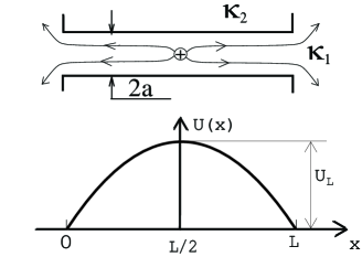
Figure 1: Electric field of a cation in a cylindrical channel with the large dielectric constant $\kappa_{1}\gg\kappa_{2}$. $L$ is the channel length, $a$ is its radius. The self–energy barrier is shown as a function of the $x$ coordinate.

Let us remind the origin of the electrostatic self–energy barrier. Consider a single cation placed in the middle of the channel with the length $L$ and the radius $a$, Fig. 1. If the ratio of the dielectric constants is large $\kappa_{1}/\kappa_{2}\gg 1$, the electric displacement $D$ is confined within the channel. As a result, the electric field lines of a charge are forced to propagate within the channel until its mouth. According to the Gauss theorem the electric field at a distance $x>a$ from the cation is uniform and is given by $E_{0}=2e/(\kappa_{1}a^{2})$. The energy of such a field in the volume of the channel is:

$$U_{L}(0)={\kappa_{1}E_{0}^{2}\pi a^{2}L\over 8\pi}={e^{2}L\over 2\kappa_{1}a^{\,2}}={eE_{0}L\over 4}\,,$$ (1)

where the zero argument is added to indicate that there are no other charges in the channel. The bare barrier, $U_{L}(0)$, is proportional to $L$ and (for a narrow channel) can be much larger than $k_{B}T$, making the channel resistance exponentially large.

Figure 2: A cation (in thin circle) bound to a negative wall charge (in thick circle). When the cation moves away from the host the energy grows linearly with the separation $|x|$.

If a dopant with the unit negative charge is attached to the inner wall of the channel it attracts a mobile cation from the salt solution (Fig. 2). There is a confining interaction potential $\Phi(x)=E_{0}|x|$ between them. Condition $e\Phi(x_{T})=k_{B}T$ defines the characteristic thermal length of such classical “atom”, $x_{T}=k_{B}T/eE_{0}=a^{2}/2l_{B}$, where $l_{B}\equiv e^{2}/(\kappa_{1}k_{B}T)$ is the Bjerrum length (for water at the room temperature $l_{B}=0.7\,$nm). This “atom” is similar to an acceptor in a semiconductor (the classical length $x_{T}$ plays the role of the effective acceptor Bohr radius). It is convenient to measure the one–dimensional concentrations of both mobile salt and dopants in units of $1/x_{T}$. In such units the small concentration corresponds to non–overlapping neutral pairs (“atoms”), while the large one corresponds to the dense plasma of mobile and immobile charges. These phases are similar to lightly and heavily doped $p$-type semiconductors, respectively.

It is important to notice that in both limits all the charges interact with each other through the 1d Coulomb potential

$$\Phi(x_{i}-x_{j})=\sigma_{i}\sigma_{j}E_{0}|x_{i}-x_{j}|,$$ (2)

where $x_{i}$ and $\sigma_{i}=\pm 1$ are coordinates and charges of both dissociated ions and dopants. Another way to formulate the same statement is to notice that the electric field experiences the jump of $2E_{0}\sigma_{i}$ at the location of the charge $\sigma_{i}$. Because all the charges inside the channel are integers in unit of $e$, the electric field is conserved modulo $2E_{0}$. It is thus convenient to define the order parameter $q\equiv\mbox{frac}[E(x)/2E_{0}]$, which is the same at every point along the channel. The physical meaning of $q\in[0,1]$ is the image charge induced in the bulk solution to terminate the electric field lines leaving the channel. One may notice that the adiabatic transport of a unit charge across the channel is always associated with $q$ spanning the interval $[0,1]$. Indeed, a charge at a distance $x$ from one end of the channel produces the fields $2E_{0}x/L$ and $2E_{0}(x/L-1)$ to the right and left of $x$, correspondingly. Therefore $q=x/L$ continuously spans the interval $[0,1]$ as the charge moves from $x=0$ to $x=L$.

To calculate the transport barrier (as well as the thermodynamics) of the channel one needs to know the free energy $F_{q}$ of the channel as a function of the order parameter. The equilibrium (referred below as the ground state) free energy corresponds to the minimum of this function $F_{\min}$. Transport of charge and thus varying $q$ within $[0,1]$ interval is associated with passing through the maximum of the $F_{q}$ function $F_{\max}$. Throughout this paper we shall refer to such a maxima as the saddle point state. The transport barrier is given by the difference between the saddle point and the ground state free energies: $U_{L}=F_{\max}-F_{\min}$. The equilibrium concentrations of ions inside the channel are given by the derivatives of $F_{\min}$ with respect to the corresponding chemical potentials related to concentrations in the bulk solution. We show below that the calculation of the partition function of the channel may be mapped on a fictitious quantum mechanical problem with the periodic potential. The function $F_{q}$ plays the role of the lowest Bloch band, where $q$ is mapped onto the quasi-momentum. As a result, the entire information of the thermodynamical as well as transport properties of the channel may be obtained from the analytical or numerical diagonalization of the proper “quantum” operator.

For an infinitely long channel with the long range interaction potential Eq. (2) we arrive at true phase transitions, in spite of the one–dimensional nature of the problem. However, at finite ratio of dielectric constants electric field lines exit from the channel at the distance $\xi\simeq a(\kappa_{1}/\kappa_{2})^{1/2}\approx 6.8\,a$. As a result, the potential Eq. (2) is truncated and phase transitions are smeared by fluctuations even in the infinite channel. In practice all the channels have finite length which leads to an additional smearing. We shall discuss sharpness of such smeared transitions below.

Figure 3: The ground state and the transport saddle point of the channel with negative monovalent dopants. Only the right part of the channel is shown. (a) The ground state ($q=0$): all dopants (thick circles) bound mobile cations (thin circles). (b) The transport saddle point ($q=1/2$): cations are free in sections between two adjacent dopants.

The outline of this paper is as follows: In section II we briefly review results for the simplest model of periodically placed negative charges in the monovalent salt solution (Fig. 3), published earlier in the short communication Zhang . In this example the barrier is gradually reduced with the increasing doping. Sections III – V are devoted to several modifications of the model which, contrary to expectations raised by the results of section II, lead to ion exchange phase transitions. In section III we consider a channel with the alternating positive and negative dopants in monovalent salt solution and study the phase transition at which mobile ions leave the channel. In section IV and V we return to equidistant negative dopants, but consider the role of divalent cations in the bulk solution. In particular, in section IV, we assume that all cations in the bulk solution are divalent and show that this does not lead to four times increase of the self–energy barrier. The reason is that the divalent ions are effectively fractionalized in two monovalent excitations. In section V we deal with a mixture of monovalent and divalent cations and study their exchange phase transition. We discuss possible implications of this transition for understanding the Ca-vs.-Na selectivity of biological Ca channels. For all the examples we present transport barrier, latent ion concentration and phase diagram along with the simple estimates, explaining the observed phenomenology. The details of the mapping onto the effective quantum mechanics as well as of the ensuing numerical scheme are delegated to sections VI and VII. Results of sections III – V are valid only for very long channels and true 1d Coulomb potential. In section VIII we discuss the effects of finite channel length and electric field leakage from the channel on smearing of the phase transitions. In section IX we consider boundary effects at the channel ends leading to an additional contact (Donnan) potential. We conclude in section X by brief discussion of possible nano-engineering applications of the presented models.

II Negatively doped channel in a monovalent solution

As the simplest example of a doped channel we consider a channel with negative unit–charge dopants periodically attached to the inner walls at distance $x_{T}/\gamma$ from each other (Fig. 3). Here $\gamma$ is the dimensionless one–dimensional concentration of dopants. At both ends (mouths) the channel is in equilibrium with a monovalent salt solution with the bulk concentration $c$. It is convenient to introduce the dimensionless monovalent salt concentration as $\alpha_{1}\equiv c\pi a^{2}x_{T}$. We shall restrict ourselves to the small salt concentration (or narrow channels) such that $\alpha_{1}\ll 1$. In this case the transport barrier of the undoped ($\gamma=0$) channel is given by Eq. (1) (save for the small screening reduction which scales as $1-4\alpha_{1}$, [Kamenev, ]).

The calculations, described in details in sections VI and VII, lead to the barrier plotted in Fig. 4 as a function of the dopant concentration $\gamma$. The barrier decreases sharply as $\gamma$ increases. For example, a very modest concentration of dopants $\gamma=0.2$ is enough to suppress the barrier more than five times (typically bringing it below $k_{B}T$). There are no phase transitions in this system in the entire phase space of concentrations $\gamma$ and $\alpha_{1}$.

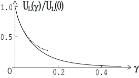
Figure 4: The function $U_{L}(\gamma)/U_{L}(0)$ for $\alpha_{1}=10^{-5}$. Its $\gamma\ll 1$ asymptotic, Eq. (5), is shown by the dotted line.

For the small dopant concentration, $\gamma\ll 1$, the result may be understood with a simple reasoning. The ground state of the channel corresponds to all negative dopants being locally neutralized by the mobile cations from the solution (Fig. 3 a). As a result, there is no electric field within the channel and thus in the ground state $q=0$. The corresponding free energy has only entropic component (the absence of the electric fields implies no energy cost) which is given by:

$$F_{0}=-\gamma Lk_{B}T\ln(2\alpha_{1})=U_{L}(0)\cdot 4\gamma\ln[1/(2\alpha_{1})]\,.$$ (3)

Indeed, bringing one cation from the bulk solution into the channel to compensate a dopant charge leads to the entropy reduction $S_{0}=k_{B}\ln(\pi a^{2}2x_{T}c)=k_{B}\ln(2\alpha_{1})$. Here $\pi a^{2}2x_{T}$ is the allowed volume of the cation’s thermal motion within the channel, while $c^{-1}$ is the accessible volume in the bulk.

The maximum of the free energy is associated with the state with $q=1/2$, see Fig. 3 b. It can be viewed as a result of putting a vacancy in the middle of the channel. The latter creates the electric field $\pm E_{0}$ which orients the dipole moments of all the “atoms”. In other words, it orders all the charges in an alternating sequence of positive and negative ones. This unbinds the cations from the dopants and makes them free to move between neighboring dopants (Fig. 3 b). Indeed, upon such rearrangement the electric field is still $E=\pm E_{0}$ everywhere in the channel, according to the Gauss theorem. Therefore, the energy of $q=1/2$ state is still given by Eq. (1). However, its entropy is dramatically increased with respect to $q=0$ state due to the unbinding of the cations: the available volume is now $\pi a^{2}x_{T}/\gamma$ and the resulting entropy per cation is $S_{1/2}=k_{B}\ln(\alpha_{1}/\gamma)$. The corresponding free energy of the saddle point state is:

$$F_{1/2}=U_{L}(0)[1-4\gamma\ln(\alpha_{1}/\gamma)]\,.$$ (4)

Recalling that the transport barrier is given by the difference between the saddle point and the ground state free energies, one obtains:

$$U_{L}(\gamma)=U_{L}(0)[1-4\gamma\ln(1/2\gamma)]\,.$$ (5)

This expression is plotted in Fig. 4 by the dotted line. It provides a perfect fit for the transport barrier at small dopant concentration. Equation (5) is applicable for $\alpha_{1}<\gamma\ll 1$. In the opposite limit $\gamma<\alpha_{1}\ll 1$ more free ions may enter the channel in the saddle point state. As a result, the calculation of $S_{1/2}$ should be slightly modified Zhang , leading to:

$$U_{L}(\gamma)=U_{L}(0)\left[1-4\gamma\ln\left({1\over 2\alpha_{1}}\sinh{\alpha_{1}\over\gamma}\right)\right]\,.$$ (6)

This result, exhibiting non–singular behavior in the small concentration limit, is valid for an arbitrary relation between $\alpha_{1}$ and $\gamma$ (both being small enough).

III Channel with alternating positive and negative dopants

As a first example exhibiting the ion–exchange (actually ion–release) phase–transition we consider a model of a “compensated” channel (the word compensation is used here by analogy with semiconductors, where acceptors can be compensated by donors). This is the channel with positive and negative unit–charge dopants alternating in one-dimensional NaCl type lattice with the lattice constant $2x_{T}/\gamma$ (Fig. 5).

Figure 5: A channel with the alternating dopants (thick circles). The mobile counterions are shown as thin circles.

The channel is filled with the solution of the monovalent salt with the bulk dimensionless concentration $\alpha_{1}=\pi a^{2}x_{T}c$. The transport barrier calculated for $\alpha_{1}=0.01$ as a function of the dopant concentration $\gamma$ is depicted in Fig. 6.

Figure 6: The transport barrier in units of $U_{L}(0)$ for the “compensated” channel of Fig. 5 for $\alpha_{1}=0.01$. The dotted line shows Eq. (10).

One observes a characteristic sharp dip in a vicinity of a certain dopant concentration $\gamma_{c}\approx 0.06$. To clarify a reason for such an unexpected behavior (cf. Fig. 4) we plot the free energy as a function of the order parameter $q$ for a few values of $\gamma$ close to $\gamma_{c}$, see Fig. 7. Notice that for small $\gamma$ the minimum of the free energy is at $q=0$, corresponding to the absence of the electric field inside the channel. The maximum is at $q=1/2$, i.e. the electric field $\pm E_{0}$. However, once the dopant concentration $\gamma$ increases the second minimum develops at $q=1/2$, which eventually overcomes the $q=0$ minimum at $\gamma=\gamma_{c}$. In the limit of large $\gamma$ the ground state corresponds to $q=1/2$ (electric field $\pm E_{0}$), while the saddle point state is at $q=0$ (no electric field). It is clear from Fig. 7 that the transition between the two limits is of the first order.

Figure 7: Free energy in units of $U_{L}(0)$ as a function of $q$ for $\gamma=0.02,~{}0.05,~{}0.07$ and $0.09$ (from top to bottom) at $\alpha_{1}=0.01$. The lower three graphs are vertically offset for clarity.

To understand the nature of this transition, consider two candidates for the ground state. The $q=0$ state, referred below as $0$, is depicted on Fig. 8 a. In this state every dopant tightly binds a counterion from the solution. Such a state does not involve an energy cost and has the negative entropy $S_{0}=k_{B}\ln(2\alpha_{1})$ per dopant. As a result, the corresponding free energy is (cf. Eq. (3)):

$$F_{0}=U_{L}(0)\cdot 4\gamma\ln[1/(2\alpha_{1})]\,.$$ (7)

An alternative ground state is that of the channel free from any dissociated ions, Fig. 8 b. There is an electric field $\pm E_{0}$ alternating between the dopants. This is $q=1/2$ state, or simply $1/2$ state. Since no mobile ions enter the channel, there is no entropy lost in comparison with the bulk. There is, however, energy cost for having electric field $\pm E_{0}$ across the entire channel. As a result, the free energy of the $1/2$ state is (cf. Eq. (1)):

$$F_{1/2}=U_{L}(0)\,.$$ (8)

Comparing Eqs. (7) and (8), one expects that the critical dopant concentration is given by

$$\gamma_{c}=-\left[4\ln(2\alpha_{1})\right]^{-1}\,.$$ (9)

For $\gamma<\gamma_{c}$ the state $0$ is expected to be the ground state, while for $\gamma>\gamma_{c}$ the state $1/2$ is preferable.

Figure 8: States $0$, $1/2$ and $00$. The corresponding free energies are given by Eqs. (7), (8) and (11).

In Fig. 9 we plot the phase diagram on the $(\gamma,~{}\alpha_{1})$ plane. The phase boundary between $0$ and $1/2$ states is determined from the condition of having two degenerate minima of the free energy $F_{q}$ at $q=0$ and $q=1/2$. In the small concentration limit (see the inset in Fig. 9) the phase boundary is indeed perfectly fitted by Eq. (9). For larger concentrations it crosses over to $\gamma_{c}\propto\sqrt{\alpha_{1}}$. This can be understood as a result of a competition between dopant separation $x_{T}/\gamma$ and the Debye screening length $r_{D}\propto x_{T}/\sqrt{\alpha_{1}}$. For $\gamma<\sqrt{\alpha_{1}}$ we have $r_{D}<x_{T}/\gamma$, and thus each dopant is screened locally by a cloud of mobile ions. As a result, the neutral state $0$ is likely to be the ground state. In the opposite case $\gamma>\sqrt{\alpha_{1}}$ the Debye length is larger than the separation between oppositely charged dopants. This is the limit of a week screening when most dopants may not have counterions to screen them. Thus the $1/2$ state has a chance to have a lower free energy.

Figure 9: The phase diagram of the channel with alternating doping (dotted lines). The phase boundary between the $q=0$ and $q=1/2$ phases can be fitted as $\alpha_{1}\approx 5\gamma^{2}$ for $\alpha_{1}>1$. Inset: the small concentration part of the phase boundary fitted by Eq. (9) (the full line).

Crossing the phase boundary in either direction is associated with an abrupt change in the one-dimensional density of the salt ions within the channel. The latter may be evaluated as the derivative of the ground state free energy with respect to the chemical potential of the salt: $n_{\mbox{ion}}=-{\alpha_{1}\over Lk_{B}T}\,{\partial F_{\min}/\partial\alpha_{1}}$. In Fig. 10 we plot concentration of ions within the channel, $n_{\mbox{ion}}$, in units of dopant concentration $\gamma/x_{T}$ as a function of the bulk salt normality $\alpha_{1}$. One clearly observes the latent concentration associated with the first-order transition. As the bulk concentration increases past the critical one, the mobile ions abruptly enter the channel. One can monitor the latent concentration $\Delta n$ along the phase transition line of Fig. 9. In Fig. 11 we plot the latent concentration along the phase boundary as function of the critical $\alpha_{1}$. As expected, in the dilute limit the latent concentration coincides with the concentration of dopants (i.e. every dopant brings one mobile ion). On the other hand, in the dense limit, the latent concentration is exponentially small (but always finite).

Figure 10: The concentration of cations inside the channel in units of $\gamma/x_{T}$ for $\gamma=0.1$. The discontinuous change occurs at the phase transition point.

Figure 11: The latent concentration of cations in units of $\gamma/x_{T}$ along the phase boundary line.

Let us return to the calculation of the transport barrier, Fig. 6. To this end one needs to understand the nature of the saddle point states (in addition to that of the ground states, discussed above). Deep in the phase where $0$ is the ground state, the role of the saddle point state is played by the $1/2$ state. Correspondingly the transport barrier is approximately given by the difference between Eq. (8) and Eq. (7). One may improve this estimate by taking into account that in the $1/2$ state the free ions may enter the channel (in even numbers to preserve the total charge neutrality). This leads to the entropy of the $1/2$ state given by $S_{1/2}=k_{B}\ln[\sum_{k=0}^{\infty}(\alpha_{1}/\gamma)^{2k}/(2k)!]$ per dopant. As a result, one finds for the transport barrier in the $0$ state:

$$U_{L}(\alpha_{1},\gamma)=U_{L}(0)\left[1-4\gamma\ln\left({1\over 2\alpha_{1}}\cosh{\alpha_{1}\over\gamma}\right)\right]\,.$$ (10)

This estimate is plotted in Fig. 6 by the dotted line.

Figure 12: Free energy diagram for $\alpha_{1}=0.01$ as function of dopant concentration $\gamma$. The solid lines are numerical results for the ground and saddle point states. Eqs. (7), (8) and (11), describing states $0$, $1/2$ and $00$, correspondingly, are shown by dashed, dotted and dash-dotted lines.

In the $1/2$ state, Fig. 8 b, the channel is almost empty in the ground state configuration. The saddle point may be achieved by putting a single cation in the middle of the channel. This will rearrange the pattern of the internal electric field as depicted in Fig. 8 c. This state corresponds to $q=0$ and is denoted as $00$ (to distinguish it from the state $0$, Fig. 8 a). Its free energy (coinciding with the energy) is given by:

$$F_{00}=2U_{L}(0)\,.$$ (11)

In Fig. 12 we plot the free energies of the three states $0$, $1/2$ and $00$ (cf. Fig. 8 and Eqs. (7), (8) and (11)) as functions of the dopant concentration $\gamma$. On the same graph we also plot the calculated ground state free energy $F_{\min}$ along with the saddle point free energy $F_{\max}$. It is clear that the ground state undergoes the first order transition between $0$ and $1/2$ states at $\gamma=\gamma_{c}$. On the other hand, the saddle point state experiences two smooth crossovers: first between $1/2$ and $0$ and second between $0$ and $00$ states. The difference between the saddle point and the ground state free energies is the transport barrier, which exhibits exactly the type of behavior observed in Fig. 6. Curiously, at large concentration of dopants the barrier approaches exactly the same value as for the undoped channel, $U_{L}(\alpha_{1})$, [Kamenev, ]. This could be expected, since extremely closely packed alternative dopants compensate each other, effectively restoring the undoped situation.

IV Negatively doped channel with divalent cations

In the above sections all the mobile ions as well as dopants were monovalent. In this section we study the effect of cations being divalent (e.g. Ca²⁺, or Ba²⁺), while all negative charges (both anions and dopants) are monovalent (Fig. 13). For example, one can imagine a channel with negative wall charges in CaCl₂ solution. We denote the dimensionless concentration of the divalent cations as $\alpha_{2}$. The concentration of monovalent anions is simply $\alpha_{-1}=2\alpha_{2}$.

Figure 13: A channel with periodic dopants (thick circles) and divalent cations. Mobile ions (Ca²⁺ and Cl^-) are in thin circles.

The transport barrier as function of the dopant concentration $\gamma$ for $\alpha_{2}=5\cdot 10^{-7}$ is shown in Fig. 14.

Figure 14: The transport barrier $U_{L}(\alpha_{2},\gamma)$ in units of $U_{L}(0)$ for $\alpha_{2}=5\cdot 10^{-7}$ (solid line). The dotted line is $|F_{1/2}-F_{0}|$, and dashed line is $|F_{00}-F_{1/2}|$ calculated using Eqs. (12), (13) and (15).

Similarly to the case of the alternating doping (cf. Fig. 6) the barrier experiences a sudden dip at some critical dopant concentration $\gamma_{c}\approx 10^{-2}$. To understand this behavior we looked at the free energy $F_{q}$ as function of the order parameter $q$ for several values of $\gamma$ in the vicinity of $\gamma_{c}$. The result is qualitatively similar to that depicted in Fig. 7. Thus, it is again the first order transition between two competing states that is responsible for the behavior observed in Fig. 14.

Figure 15: The states $0$, $1/2$, and $00$ for the channel with divalent cations. The corresponding free energies are given by Eqs. (12), (13) and (15). Dopants (thick circles) and anions (thin circles) are monovalent, while cations (shown by $2+$ in thin circles) are divalent. Electric fields are shown schematically, one line per $E_{0}$.

The two candidates for the ground state, denoted, in accordance with the fractional part of the internal electric field $q$, as $0$ and $1/2$, are depicted in Fig. 15 a,b. In the state $0$ every dopant is screened locally by an anion and a doubly charged cation (Fig. 15 a). The corresponding free energy (consisting solely from the entropic part) is given by ft6 :

$$F_{0}=U_{L}(0)\cdot 4\gamma\ln\left({1\over 6\alpha_{2}^{2}}\right).$$ (12)

The other state, $1/2$, has every second dopant overscreened by a divalent cation (Fig. 15 b). The free energy of this state is:

$$F_{1/2}=U_{L}(0)\left[1+{4\gamma\over 2}\ln(1/\alpha_{2})\right]\,.$$ (13)

Comparing Eqs. (12) and (13), one finds for the critical dopant concentration:

$$\gamma_{c}=-\left[6\ln(\alpha_{2})+4\ln 6\right]^{-1}\,.$$ (14)

For $\alpha_{2}=5\cdot 10^{-7}$ it leads to $\gamma_{c}\approx 0.012$ in a good agreement with Fig. 14.

To explain the transport barrier observed for small $\gamma$ (Fig. 14) one needs to know the saddle point state. Such a state is depicted in Fig. 15 c and is denoted as $00$. It has one divalent cation trapped between every other pair of dopants. It is easy to see that for such arrangement the cations are free to move within the “cage” defined by the two neighboring dopants. This renders a rather large entropy of the $00$ state. Its free energy is given by

$$F_{00}=U_{L}(0)\left[2+{4\gamma\over 2}\ln({\gamma/\alpha_{2}})\right]\,.$$ (15)

In Fig. 16 we plot the free energies of the states $0$, $1/2$ and $00$, given by Eqs. (12), (13) and (15) correspondingly, as functions of $\gamma$. On the same graph we plot calculated ground state free energy $F_{\min}$ along with the saddle point free energy $F_{\max}$ (full lines). One observes that the ground state indeed undergoes the first order transition between the states $0$ and $1/2$ upon increasing $\gamma$ (lower full line). On the other hand, the saddle point evolves smoothly from $1/2$ to $0$ and eventually to $00$ (upper full line). The difference between the two gives the transport barrier depicted in Fig. 14, where $|F_{1/2}-F_{0}|$ and $|F_{00}-F_{1/2}|$ are also shown for comparison.

Figure 16: Free energy diagram for $\alpha_{2}=5\cdot 10^{-7}$ as a function of dopant concentration $\gamma$. The full lines are numerical results for the ground and saddle point states respectively. Eqs. (13), (15) and (12) describing states $1/2$, $00$ and $0$, are shown by dashed, dash-dotted and solid thin line correspondingly. State $0$ is the ground state for $\gamma<\gamma_{c}$, state $1/2$ is the ground state for $\gamma>\gamma_{c}$, and the state $00$ is the saddle point for $\gamma>\gamma_{c}^{\prime}$. The ground state undergoes the first order phase transition at $\gamma_{c}$, while the saddle point state evolves in a continuous way.

It is worth noticing that on the both sides of the transition the transport barrier is close to $U_{L}(0)$, characteristic for the transfer of the unit charge $e$. One could expect that for charges $2e$ the self-energy barrier should be rather $4U_{L}(0)$. This apparent reduction of the charge seems natural for the very small $\gamma$. Indeed, the corresponding ground state (Fig. 15 a) contains complex ions (CaCl)¹⁺ with the charge $e$. On the other hand, for $\gamma>\gamma_{c}$ the channel is free from Cl^- ions and the current is provided by Ca²⁺ ions only. Thus, the observed barrier of $\leq U_{L}(0)$ may be explained by fractionalization of charges $2e$ into two charges $e$. To make such a fractionalization more transparent one can redraw the saddle point state $00$ in a somewhat different way, namely creating a soliton (domain wall, or defect) in the state $1/2$.

Fig. 17 shows the channel with a soliton in the middle.

Figure 17: The saddle point state $00$ represented as the unit charge defect (soliton) within the ground state $1/2$. Ca²⁺ ion added to the channel in the state $1/2$ fractionalizes in two such solitons, each having an excess energy $\leq U_{L}(0)$.

One can see that in this version of the $00$ state the fields $2E_{0}$ and $0$ alternate similarly to Fig. 15 c. We can also see that the soliton in the middle has the charge $e$. Fractionalization of a single Ca²⁺ ion in two charge–$e$ defects means that a Ca ion traverses the channel by means of two solitons moving consecutively across the channel. The self-energy of each soliton (and therefore the transport barrier) does not exceed $U_{L}(0)$.

Figure 18: $\ln[U_{L}(\gamma)/U_{L}(0)]$ for $\alpha_{2}=5*10^{-5}$. Each dip signals the presence of a phase transition.

Figure 19: The phase diagram of the channel with the divalent cations on the $(\gamma,~{}\alpha_{2})$ plane. The dotted lines are the boundaries between phases. The ground states in each region are labelled. Inset: magnification of the first phase boundary line at small $\gamma$. The solid line is Eq. (14).

So far the physics of the first order transition in the divalent system was rather similar to that in the channel with the alternating doping and a monovalent salt. There are, however, important distinctions, taking place at larger dopant concentration. The logarithm of the transport barrier in the wide range of $\gamma$ is plotted in Fig. 18. One notices a series of additional dips at $\gamma_{c1}\approx 1.7$, $\gamma_{c2}\approx 5.3$, $\gamma_{c3}\approx 10.8$, etc. (the first order transition at $\gamma_{c}\approx 0.01$, discussed above, is not visible at this scale). These dips are indications of the sequence of reentrant phase transitions, taking place at larger $\gamma$. The calculated phase diagram is plotted in Fig. 19. The leftmost phase boundary line corresponds to the first order phase transition between $0$ and $1/2$ states. Its low concentration part along with the fit with Eq. (14) is magnified in the inset. The other lines are transitions spotted in Fig. (18). We discuss them in Appendix A.

V negatively doped Channel in solution with monovalent and divalent cations

We turn now to the study of the channel in a solution with the mixture of monovalent cations with the dimensionless concentration $\alpha_{1}$ and divalent cations with the concentration $\alpha_{2}$. Neutrality of the solution is maintained by monovalent anions with the concentration $\alpha_{-1}=\alpha_{1}+2\alpha_{2}$. The channel is assumed to be doped with the unit charge negative dopants, attached periodically with the concentration $\gamma$.

In Fig. 20 we plot the barrier as a function of the divalent cation concentration $\alpha_{2}$ for $\gamma=0.1$ and $\alpha_{1}=0.001$.

Figure 20: The transport barrier as a function of $\ln\alpha_{2}$ for $\gamma=0.1$ and $\alpha_{1}=0.001$.

The overall decrease of the barrier with the growing ion concentration is interrupted by the two sharp dips at $\alpha_{2c}$ and $\alpha_{2c}^{\prime}$. By plotting the $F_{q}$ function for several $\alpha_{2}$ in the vicinity of $\alpha_{2c}$ and $\alpha_{2c}^{\prime}$, one observes that they correspond to the two consecutive first order transitions. As $\alpha_{2}$ increases the system goes from $q=0$ phase into $q=1/2$ phase and eventually back into $q=0$ phase.

Figure 21: Concentration of Ca²⁺ ions in the channel in units of $\gamma/x_{T}$ as function of $\ln\alpha_{2}$ for $\gamma=0.1$ and $\alpha_{1}=0.001$. There are two discontinuous changes in Ca concentration at $\alpha_{2c}$ and $\alpha_{2c}^{\prime}$. Each of these two latent changes is close to the half of the number of dopants.

The concentration of divalent cations within the channel is given by

$$n_{{Ca}}=-{\alpha_{2}\over k_{B}TL}\,\left.{\partial F_{\min}\over\partial\alpha_{2}}\right|_{\alpha_{1},\alpha_{-1}}.$$ (16)

It is plotted as a function of the bulk concentration in Fig. 21. One observes that at the first transition the number of divalent cations entering the channel is close to the half of the number of dopants. When the second transition is completed the number of divalent cations is approximately the same as the number of dopants. This provides a clue on the nature of the corresponding ground states. For $\alpha_{2}<\alpha_{2c}$ there are almost no divalent cations in the channel. Therefore, both the ground state and the saddle point state are the same as in sec. II, shown in Fig. 3. The ground state free energy and the transport barrier are given by Eqs. (3) and (5) correspondingly. At $\alpha_{2}=\alpha_{2c}$ the first order ion–exchange phase transition takes place, where every two monovalent cations are getting substituted by a single divalent one. The system’s behavior at larger $\alpha_{2}$ is qualitatively similar to that described in the previous section. For $\alpha_{2c}<\alpha_{2}<\alpha_{2c}^{\prime}$ the ground state is the $1/2$ state, pictured in Fig. 15 b. The corresponding free energy is given by Eq. (13). The second phase transition at $\alpha_{2c}^{\prime}$ is similar to that taking place on the leftmost phase boundary of Fig. 19 (which is crossed now in the vertical direction). For $\alpha_{2}>\alpha_{2c}^{\prime}$ the ground state is the state $0$ (Fig. 15 a) with the free energy given by Eq. (12).

Figure 22: Free energies of the three competing ground states for $\gamma=0.1$ and $\alpha_{1}=0.001$. The dash-dotted line is Eq. (3), the solid line is Eq. (13), and the dashed line is Eq. (12). The actual ground state is chosen as the lowest of them.

The free energies of the three competing ground states as functions of $\alpha_{2}$ are plotted in Fig. 22 for the same parameters as in Fig. 20. They indeed intersect at the concentrations close to $\alpha_{2c}$ and $\alpha_{2c}^{\prime}$. Since at each such intersection the symmetry of the ground state (the $q$-value) changes, one expects that the ground state changes via the first-order phase transition. The critical value $\alpha_{2c}$ of the ion–exchange transition may be estimated from Eqs. (13) and (3) as:

$$\alpha_{2c}=(2\alpha_{1})^{2}e^{1/(2\gamma)}\,.$$ (17)

Notice that it scales as $\alpha_{1}^{2}$ and therefore at small concentrations the transition takes place at $\alpha_{2c}\ll\alpha_{1}$. This is a manifestation of the law of mass action. The second critical value may be estimated from Eq. (14) as $\alpha_{2c}^{\prime}=e^{-1/(6\gamma)}$ and is approximately independent on $\alpha_{1}$. Comparing the two, one finds that the transitions may take place only for small enough concentration of the monovalent ions $\ln\alpha_{1}\lesssim-\gamma/3-\ln 2$. For larger $\alpha_{1}$ there is a smooth crossover between the two $q=0$ states.

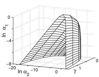
Figure 23: Phase diagram in the space of cation and dopant concentrations ($\ln\alpha_{2}-\gamma-\ln\alpha_{1}$). Inside the tent-like shape the ground state is $q=1/2$, outside – the ground state is $q=0$.

The phase diagram in the space of cation and dopant concentrations ($\ln\alpha_{2}-\gamma-\ln\alpha_{1}$) is plotted in Fig. 23. By fixing some $\gamma$ and not too large $\alpha_{1}$ and varying $\alpha_{2}$ one crosses the phase boundary twice. This way one observes two first order phase transitions: from $0$ to $1/2$ and then from $1/2$ to $00$. The corresponding transport barrier is shown in Fig. 20.

Figure 24: Schematic plot of the current through a Ca channel as a function of Ca²⁺ concentration, cf. Ref. Almers, . The Na⁺ concentration is $\alpha_{1}\approx 10^{-2}$, the wall charge concentration is $\gamma\approx 0.3$, and the (smeared) transition is at $\ln\alpha_{2c}\approx-10$.

The model presented in this section is a simple cartoon for Ca²⁺ selective channels. Let us consider the total current through the channel, $I$, equal to the sum of sodium and calcium currents. Each of these partial currents in turn is determined by two series resistances: the channel resistance and the combined contact (mouth) resistances (the latter are inversely proportional to the concentration of a given cation in the bulk). We assume that at the biological concentration of Na⁺ the current $I=I_{0}$ and discuss predictions of our model of negatively doped channel at $\gamma\approx 0.3$ regarding $I/I_{0}$ with growing concentration $\alpha_{2}$ of Ca²⁺ cations (Fig. 24). For $\alpha_{2}<\alpha_{2c}$ the channel is populated by Na⁺ and Na⁺ current dominates. For $\alpha_{2}>\alpha_{2c}$ the Na⁺ current is blocked because Na⁺ ions are expelled from the channel and substituted by the Ca²⁺. Indeed, a monovalent Na⁺ cation cannot unbind the divalent Ca²⁺ from the dopants. Therefore, the transport barrier for Na⁺ ions is basically the bare barrier $U_{L}(0)\gg k_{B}T$. In these conditions the Ca²⁺ resistance of the channel is small, because Ca²⁺ concentration in the channel is large. However, at the transition $\alpha_{2}=\alpha_{2c}\ll\alpha_{1}$ the concentration of Ca²⁺ ions in the bulk water is so small that the contact Ca²⁺ resistance is very large. Therefore, the Ca²⁺ current is practically blocked and the total current, $I$, drops sharply at $\alpha_{2c}$. As $\alpha_{2}$ grows the Ca²⁺ current increases proportional to $\alpha_{2}$ due to decreasing contact resistance. As a result, one arrives at the behavior of $I/I_{0}$ schematically shown in Fig. 24. This behavior is in a qualitative agreement with the experimental data of Refs. [Almers, ; Hille, ].

VI Analytical approach

Consider a gas consisting of $N$ mobile monovalent cations and $N^{\prime}$ mobile monovalent anions along with non–integer boundary charges $q$ and $q^{\prime}$ placed at $x=0$ and $x=L$ correspondingly. We also consider a single negative unit dopant charge attached at the point $x_{0}$ inside the channel: $0<x_{0}<L$. The resulting charge density takes the form:

$$\rho(x)\equiv\!\!\sum\limits_{j=1}^{N+N^{\prime}}\!\!\sigma_{j}\delta(x-x_{j})+q\delta(x)+q^{\prime}\delta(x-L)-\delta(x-x_{0})\,,$$ (18)

where $x_{j}$ stay for coordinates of the mobile charges and $\sigma_{j}=\pm 1$ for their charges. The interaction energy of such a plasma is given by:

$$U={e\over 2}\int\!\!\!\int\limits_{0}^{L}\!\!dxdx^{\prime}\rho(x)\Phi(x-x^{\prime})\rho(x^{\prime})\,,$$ (19)

where the 1d Coulomb potential $\Phi(x)=\Phi(0)-E_{0}|x|$ is the solution of the Poisson equation: $\nabla^{2}\Phi=-2E_{0}\delta(x)$. (The self-energy $e\Phi(0)$ will be eventually taken to infinity to enforce charge neutrality).

We are interested in the grand-canonical partition function of the gas defined as

$$Z_{L}(q,q^{\prime})=\sum\limits_{N,N^{\prime}=0}^{\infty}e^{\mu(N+N^{\prime})/(k_{B}T)}{1\over N!N^{\prime}!}$$ (20)

$$\times\prod\limits_{j=1}^{N+N^{\prime}}\left({\pi a^{\,2}\over l_{0}^{2}}\int\limits_{0}^{L}{dx_{j}\over l_{0}}\right)e^{-U/(k_{B}T)}\,,$$

where $\mu$ is the chemical potential (the same for cations and anions) and $l_{0}$ is a microscopic scale related to the bulk salt concentration as $c=e^{\mu/k_{B}T}/l_{0}^{3}$. Factor $\pi a^{2}/l_{0}^{2}$ originates from the integrations over transverse coordinates.

To proceed with the evaluation of $Z_{L}(q,q^{\prime})$ we introduce the resolution of unity written in the following way:

$$1 = \int\!\!{\cal D}\!\rho(x)\,\,\delta\!\!\left(\rho(x)-\sum\limits_{j=1}^{N+N^{\prime}}\sigma_{j}\delta(x-x_{j})-q\delta(x)-q^{\prime}\delta(x-L)+\delta(x-x_{0})\right)$$

$$= \int\!\!\!\int{\cal D}\!\rho(x){\cal D}\theta(x)\,\,\exp\left\{\,-i\left(\int\limits_{0}^{L}\!dx\,\theta(x)\rho(x)-\sum\limits_{j=1}^{N+N^{\prime}}\sigma_{j}\theta(x_{j})-q\theta(0)-q^{\prime}\theta(L)+\theta(x_{0})\right)\right\}~{}.$$

Substituting this identity into Eq. (20), one notices that the integrals over $x_{j}$ decouple and can be performed independently. The result of such integration along with the summation over $N$ and $N^{\prime}$ is $\exp\{2\pi a^{2}c\int_{0}^{L}dx\cos\theta(x)\}$. Evaluation of the Gaussian integral over $\rho(x)$ yields the exponent of $\theta(x)\Phi^{-1}(x-x^{\prime})\theta(x^{\prime})$. According to the Poisson equation the inverse potential is $\Phi^{-1}(x-x^{\prime})=-(2E_{0})^{-1}\delta(x-x^{\prime})\partial^{2}_{x}$. As a result, one obtains for the partition function:

$$Z(q,q^{\prime})= \int\!\!\!\!\int\limits_{-\infty}^{\infty}\frac{d\theta_{0}d\theta_{L}d\theta_{x_{0}}}{(2\pi)^{3}}\,\,e^{iq\theta_{i}+iq^{\prime}\theta_{f}-i\theta_{x_{0}}}\int\!\!{\cal D}\theta(x)\,\,\exp\left\{-\int\limits_{0}^{L}\!\!dx\left[{x_{T}\over 4}(\partial_{x}\theta)^{2}-{2\alpha_{1}\over x_{T}}\cos\theta(x)\right]\right\}\,,$$

where $\alpha_{1}=\pi a^{2}x_{T}c$. The integral over $\theta(x)$ runs over all functions with the boundary conditions $\theta(0)=\theta_{0}\,$, $\theta(L)=\theta_{L}$ and $\theta(x_{0})=\theta_{x_{0}}$.

It is easy to see that this expression represents the matrix element of the following T-exponent (or rather X-exponent) operator:

$$Z(q,q^{\prime})=\langle q|e^{-{x_{0}\over x_{T}}\,\hat{H}}e^{-i\theta}e^{-{L-x_{0}\over x_{T}}\,\hat{H}}|q^{\prime}\rangle\,,$$ (21)

where the Hamiltonian is given by $\hat{H}=(i\hat{\partial}_{\theta})^{2}-2\alpha_{1}\cos\theta$ and $|q\rangle$ is the eigenstate of the momentum operator $i\hat{\partial}_{\theta}$. Since the Hamiltonian conserves the momentum up to an integer value, $q^{\prime}=q+M$, one can restrict the Hilbert space down to the subspace with the fixed fractional part of the boundary charge $0\leq q<1$. In this subspace one can perform the gauge transformation, resulting in the Mathieu Hamiltonian with the “vector potential” Lenard ; Edwards ; Kamenev :

$$\hat{H}_{q}=(i\hat{\partial}_{\theta}-q)^{2}-2\,\alpha_{1}\cos\theta\,.$$ (22)

It acts in the space of periodic functions: $\Psi(\theta)=\Psi(\theta+2\pi)$. Finally, taking the “democratic” sum over all integer parts of the boundary charge (with the fixed fractional part $q$), one obtains:

$$Z(q)=\mbox{Tr}\left\{e^{-\hat{H}_{q}{x_{0}\over x_{T}}}\,e^{-i\theta}\,e^{-\hat{H}_{q}{L-x_{0}\over x_{T}}}\right\}\,.$$ (23)

In the more general situation the solution contains a set of ions with charges (valences) $m\in{\cal Z}$ and the corresponding dimensionless concentrations $\alpha_{m}$. The condition of total electro-neutrality demands that:

$$\sum\limits_{m}m\,\alpha_{m}=0\,.$$ (24)

The Mathieu Hamiltonian (22) should be generalized as Edwards :

$$\hat{H}_{q}=(i\hat{\partial}_{\theta}-q)^{2}-\sum\limits_{m}\alpha_{m}\,e^{im\theta}\,.$$ (25)

Despite of being non–Hermitian, this Hamiltonian still possesses a real band–structure ftnt $\epsilon_{q}^{(j)}$. It is safe to assume that monovalent anions are always present in the solution: $\alpha_{-1}>0$. This guarantees that the band–structure has the unit period in $q$.

Consider first an undoped channel. Its partition function is given by $Z(q)=\mbox{Tr}\{\exp(-\hat{H}_{q}L/x_{T})\}$. In the long channel limit, $L\gg x_{T}$, only the ground state, $\epsilon^{(0)}_{q}$, of the Hamiltonian (22) or (25) contributes to the partition function. As a result, the free energy of the 1d plasma is given by

$$F_{q}=k_{B}T\epsilon^{(0)}_{q}(\alpha_{m})L/x_{T}=4U_{L}(0)\epsilon^{(0)}_{q}(\alpha_{m})\,.$$ (26)

The equilibrium ground state of the plasma corresponds to the minimal value of the free energy. For the Mathieu Hamiltonian (22) $\epsilon^{(0)}_{q}$ has a single minimum at $q=0$ (no induced charge at the boundary). It is also the case for the more general Hamiltonians (25). Therefore the equilibrium state of a neutral 1d Coulomb plasma does not have a dipole moment and possesses the reflection symmetry.

The adiabatic transfer of the unit charge across the channel is associated with the slow change of $q$ from $q=0$ to $q=\pm 1$. In this way the system must overcome the free energy maximum at some value of $q$ (for the operators (22) and (25) the maximum is at $q=1/2$). As a result, the activation barrier for the charge transfer is proportional to the band-width of the lowest Bloch band Kamenev :

$$U_{L}(\alpha_{m})=4U_{L}(0)\left(\epsilon^{(0)}_{\mbox{max}}(\alpha_{m})-\epsilon^{(0)}_{\mbox{min}}(\alpha_{m})\right)\,.$$ (27)

Notice that in the ideal 1d Coulomb plasma the transport barrier scales as the system size. It is also worth mentioning that both the equilibrium free energy $F_{0}=4U_{L}(0)\epsilon^{(0)}_{\mbox{min}}(\alpha_{m})$ and the transport barrier, Eq. (27), are smooth analytic functions of the concentrations $\alpha_{m}$. Since there is the unique minimum and maximum within the interval $0\leq q<1$, there are no phase transitions in the undoped channels.

Most of biological ion channels have internal “doping” wall charges within the channel. If integer charges $n_{1},n_{2},\ldots,n_{N}$ are fixed along the channel at the coordinates $0<x_{1}<x_{2}<\ldots<x_{N}<L$, the partition function is obtained by straightforward generalization of Eq. (23):

$$Z(q)=\mbox{Tr}\left\{e^{-\hat{H}{x_{1}\over x_{T}}}e^{in_{1}\theta}e^{-\hat{H}{x_{2}-x_{1}\over x_{T}}}\ldots e^{in_{N}\theta}e^{-\hat{H}{L-x_{N}\over x_{T}}}\right\}\,.$$ (28)

As long as all $n_{k}$ are integer, the boundary charge $q$ is a good quantum number of the operator under the trace sign. As a result, the partition function is again a periodic function of $q$ with the unit period.

For the sake of illustration we shall focus on systems with periodic arrangements of the wall charges. In this case the partition function (28) takes the form: $Z(q)=\mbox{Tr}\{\left(\hat{\cal U}_{q}\right)^{N}\}$, where $N$ is the number of dopants in the channel and $\hat{\cal U}_{q}$ is the single–period evolution operator. We shall define the spectrum of this operator as:

$$\hat{\cal U}_{q}\,\Psi^{(j)}_{q}(\theta)=e^{-\epsilon_{q}^{(j)}/\gamma}\,\Psi^{(j)}_{q}(\theta)\,,$$ (29)

where $\gamma$ is the dimensionless concentration of dopants, defined as $\gamma\equiv x_{T}N/L$. The evolution operator $\hat{\cal U}_{q}$ is non–Hermitian. Its spectrum is nevertheless real and symmetric function of $q$. The proof of this statement may be constructed in the same way as for the operator in Eq. (25) ftnt . The free energy of a long doped system is given by $F_{q}=k_{B}T\epsilon_{q}^{(0)}N/\gamma=4U_{L}(0)\epsilon_{q}^{(0)}$ (cf. Eq. (26)). The equilibrium ground state is given by the absolute minimum of this function. Similarly, the transport barrier is given by Eq. (27).

The simplest example is the periodic sequence of unit–charge negative dopants ($x_{k+1}-x_{k}=L/N$ and $n_{k}=-1$) in the monovalent salt solution, section II. The single–period evolution operator takes the form:

$$\hat{\cal U}_{q}=e^{-i\theta}e^{-\hat{H}_{q}/\gamma}\,,$$ (30)

with $\hat{H}_{q}$ given by Eq. (22). As shown in Ref. Zhang, its ground state $\epsilon_{q}^{(0)}(\alpha_{1},\gamma)$ is a function qualitatively similar to the lowest Bloch band of the Mathieu operator in Eq. (22). As a result, both equilibrium free energy and the transport barrier are smooth function of the salt concentration $\alpha_{1}$ and the dopant concentration $\gamma$.

The examples of sections IV and V are described by the evolution operators, which have the form of Eq. (30) with the generalized Hamiltonian, Eq. (25). In the example of section IV there are two non-zero concentrations: $\alpha_{-1}=2\alpha_{2}$, while in section V one deals with three types of ions: $\alpha_{-1}=\alpha_{1}+2\alpha_{2}$. Finally, the alternating doping example of section III is described by the evolution operator of the form

$$\hat{\cal U}_{q}=e^{-i\theta}e^{-\hat{H}_{q}/\gamma}e^{+i\theta}e^{-\hat{H}_{q}/\gamma}$$ (31)

with the Hamiltonian (22). Such operators may have more complicated structure of their lowest Bloch band. In particular, the latter may have more than one minimum within the period of the reciprocal lattice: $q\in[0,1]$. The competition between (and splitting of) the minima results in the first (second) order phase transitions.

The analytic investigation of the spectrum of the evolution operators, such as Eq. (30), is possible in the limits of small and large dopant concentrations $\gamma$. For $\gamma\ll 1$ it follows from Eq. (30) that only the lowest eigenvalues of $\hat{H}_{q}$ are important. It is then enough to keep only the ground state of $\hat{H}_{q}$, save for an immediate vicinity of $q=1/2$, where the ground and the first excited states may be nearly degenerate. If also $\alpha_{m}\ll 1$ the spectrum of $\hat{H}_{q}$ along with the matrix elements of $e^{\pm i\theta}$ may be calculated in the perturbation theory. Such calculations lead to the free energies of the ground and saddle point states, which are identical to those derived in sections II–V using simple energy and entropy counting.

In the limit $\gamma\gg 1,\alpha_{m}$ one may develop a variant of the WKB approximation in the plane of the complex $\theta$, Zhang . It shows that the transport barrier and latent concentration scales as $\exp\{-c\sqrt{\gamma}\}$, where non-universal numbers $c$ are given by certain contour integrals in the complex plane of $\theta$. In the example of section II we succeeded in quantitative prediction of the coefficient $c$, see Ref. [Zhang, ]. In the case of the section IV the coefficient in front of $\cos(2\pi q)$ (see Eq. (39)) is an oscillatory function of $\gamma$. This probably translates into the complex value of the corresponding $c$–constant. We did not succeed, however, in its analytical evaluation.

VII Numerical calculations

By far the simplest way to find the spectrum of $\hat{\cal U}_{q}$ is numerical. In the basis of the angular momentum $e^{ik\theta}$ the Hamiltonian (25) takes the form of the matrix:

$$\left[\hat{H}_{q}\right]_{k,k^{\prime}}=\left[(k+q)^{2}\delta_{k,k^{\prime}}-\sum\limits_{m}\alpha_{m}\delta_{k,k^{\prime}+m}\right]\,.$$ (32)

In the same basis the dopant charge $n$ creation operator takes the matrix form: $\left[e^{in\theta}\right]_{k,k^{\prime}}=\left[\delta_{k,k^{\prime}+n}\right]$, where $k=\ldots,-2,-1,0,1,2,\ldots$ . Truncating these infinite matrices with some large cutoff, one may exponentiate the Hamiltonian and obtain the matrix form of $\left[\hat{\cal U}_{q}\right]_{k,k^{\prime}}$. The latter may be numerically diagonalized to find the function $\epsilon^{(0)}_{q}(\alpha_{m},\gamma)$. The free energy and the transport barrier are then given by Eqs. (26) and (27).

We start from the simplest case of section II. The monovalent salt with the concentration $\alpha_{-1}=\alpha_{1}$ leads to the term $-\alpha_{1}\delta_{k,k^{\prime}+1}-\alpha_{1}\delta_{k,k^{\prime}-1}$ in the matrix $\left[\hat{H}_{q}\right]$. For illustration we show the $4\times 4$ truncation of $\left[\hat{H}_{q}\right]$ and $\left[e^{-i\theta}\right]$ matrices $\left[\hat{H}_{q}\right]\rightarrow\left(\begin{array}[]{clcr}(1+q)^{2}&-\alpha_{1}&0&0\\ -\alpha_{1}&(0+q)^{2}&-\alpha_{1}&0\\ 0&-\alpha_{1}&(-1+q)^{2}&-\alpha_{1}\\ 0&0&-\alpha_{1}&(-2+q)^{2}\\ \end{array}\right)$ and $\left[e^{-i\theta}\right]\rightarrow\left(\begin{array}[]{clcr}0&1&0&0\\ 0&0&1&0\\ 0&0&0&1\\ 0&0&0&0\\ \end{array}\right)$. For reasonable precision the truncation size of the numerical calculation has to be much larger. Typically we used $40\times 40$ and checked that a further increase does not affect the results.

To calculate the “energy” band $F_{q}$ of a long channel for certain $\alpha_{1}$ and $\gamma$ one can use the matrix form of $\hat{H}_{q}$ and $e^{-i\theta}$, equate the largest eigenvalue of $\hat{\cal U}_{q}$ in Eq. (30) to $e^{-\epsilon^{(0)}_{q}/\gamma}$, and calculate $F_{q}=k_{B}T\epsilon^{(0)}_{q}L/x_{T}$. Such a calculation gives the transport barrier $U_{L}(\alpha_{1},\gamma)\equiv F_{max}-F_{min}$ shown in Fig. 4.

The models in sections IV and V are treated similarly, except that they have salt ion terms $-{\alpha_{2}}\delta_{k,k^{\prime}+2}-2\alpha_{2}\delta_{k,k^{\prime}-1}$ and$-\alpha_{1}\delta_{k,k^{\prime}+1}-\alpha_{2}\delta_{k,k^{\prime}+2}-(\alpha_{1}+2\alpha_{2})\delta_{k,k^{\prime}-1}$ respectively in $\left[\hat{H}_{q}\right]$. For the model of section III, $\left[\hat{H}_{q}\right]$ contains salt ion term $-\alpha_{1}\delta_{k,k^{\prime}+1}-\alpha_{1}\delta_{k,k^{\prime}-1}$. However, $\hat{\cal U}_{q}$ is of the form of Eq. (31) and its largest eigenvalue is denoted as $e^{-2\epsilon^{(0)}_{q}/\gamma}$.

VIII Effects of the finite length and the electric field escape

The consideration of the previous sections was certainly an idealization that neglected several important phenomena. The most essential of them are: (i) the finite length $L$ of the channel; (ii) the escape of the electric field lines from the water into the media with smaller dielectric constant. Each of these phenomena leads to a smearing of the ion-exchange phase transitions transforming them into crossovers. The goal of this section is to estimate the relative sharpness of these crossovers.

Consider first the effect of the finite length (still neglecting the field escape). Close to the first order phase transition the free energy admits two competing minima (typically at $q=0$ and $q=1/2$) with the free energies $F_{0}(\alpha_{1})$ and $F_{1/2}(\alpha_{1})$, see Fig. 7 (we focus on the alternating dopants example of section III). Being an extensive quantity, the free energy is proportional to the channel length: $F_{b}\propto L$, where $b=0,1/2$. Each of these two minima is characterized by a certain ion concentration $n_{b}(\alpha_{1})=-\alpha_{1}/(k_{B}TL)\partial F_{b}/\partial\alpha_{1}$. In the vicinity of the phase transition at $\alpha=\alpha_{c}$ the difference of the two free energies may be written as:

$$\frac{F_{0}(\alpha_{1})-F_{1/2}(\alpha_{1})}{k_{B}T}=\Delta n_{\mbox{ion}}L\,\frac{\alpha_{1}-\alpha_{c}}{\alpha_{c}}\,,$$ (33)

where $\Delta n_{\mbox{ion}}=n_{0}(\alpha_{c})-n_{1/2}(\alpha_{c})$ is the latent concentration of ions across the transition. Taking a weighted sum of the two states, one finds that the concentration change across the transition is given by the “Fermi function”:

$$\Delta n(\alpha_{1})=\frac{\Delta n_{\mbox{ion}}}{e^{\Delta N(\alpha_{c}-\alpha_{1})/\alpha_{c}}+1}\,,$$ (34)

where $\Delta N\equiv\Delta n_{\mbox{ion}}L$ is the total latent amount of ions in the finite length channel. This gives for the transition width $(\alpha_{1}-\alpha_{c})/\alpha_{c}\propto 1/\Delta N$. Therefore the transition is relatively sharp as long as $\Delta N\gg 1$. For small enough $\gamma$ the number of ions entering or leaving the channel at the phase transition is almost equal to the number of dopants: $\Delta N\lesssim N_{\mbox{dopants}}=\gamma L/x_{T}$. The necessary condition of having a sharp transition, therefore, is to have many dopants inside the channel. For example, for the transition of Fig. 10 $\Delta n_{\mbox{ion}}\approx 0.8\gamma/x_{T}$ and $\gamma=0.1$, one finds $\Delta N\approx 0.08L/x_{T}$. At larger $\gamma$ the number of dopants increases (for fixed length $L$), but the relative latent concentration is rapidly decreasing, see Fig. 11. Employing Eq. (9), one estimates $\Delta N\approx\gamma(1-2e^{-1/(4\gamma)})L/x_{T}$ this expression is maximized at $\gamma\approx 0.15$, where $\Delta N\approx 0.1L/x_{T}$. We notice, in passing, that even for $\Delta N\lesssim 1$, being plotted as a function of $\log\alpha_{2}$, the function (37) still looks as a rather sharp crossover.

Figure 25: Electrostatic potential $\Phi(x)$ in units of $e/\kappa_{1}a$ of a point charge in an infinitely long channel as a function of the dimensionless distance $x/a$ along the channel axis. Here $a$ is the radius of the cylinder, and $\kappa_{1}/\kappa_{2}=40$. The full line is an exact solution of the Laplace equation Smythe ; Parsegian . The dotted lines are 3d Coulomb potentials: the lower one is $-e/\kappa_{1}x$; the upper one is $\Phi_{\infty}-e/\kappa_{2}x$, where $e\Phi_{\infty}=2U_{\infty}$ and $U_{\infty}$ is the self-energy of a charge in the infinite channel. The dashed line corresponds to Eq.35.

We turn now to the discussion of the electric field escape from the channel, which happens due to the finite ratio of the dielectric constants of the channel’s interior, $\kappa_{1}$, and exterior, $\kappa_{2}$. Fig. 25 shows the electrostatic potential of a unit point charge placed in the middle of the channel with $\kappa_{1}/\kappa_{2}=40$, [Smythe, ]. The potential interpolates between $-e/(\kappa_{1}x)$ at small distances, $x\lesssim a$, and $2U_{\infty}/e-e/\kappa_{2}x$, where $U_{\infty}=e^{2}\xi/(\kappa_{1}a^{2})$, at large distances $x>\xi$. Here the length scale $\xi\simeq a\sqrt{\kappa_{1}/\kappa_{2}}\approx 6.8a$ is the characteristic escape length of the electric field displacement from the interior of the channel into the surrounding media with the smaller dielectric constant. The quantity $U_{\infty}=U_{L}(0)2\xi/L$ is the excess self-energy of bringing a unit charge inside the infinite channel.

In between the two limits the potential may be well approximated by the following phenomenological expression (dashed line in Fig. 25):

$$\Phi(x)=E_{0}\xi\left[1-e^{-|x|/\xi}-1.1\,{a\over\xi}\right]\,.$$ (35)

Our previous considerations correspond to the limit $\xi\to\infty$ (save for the last term). The last term in Eq. (35) originates from the fact that in the immediate vicinity of the charge $|x|\lesssim a$ the electric field is not disturbed by the presence of the channel walls. As a result the length of $\approx 1.1a$ is excluded from paying the excess self-energy price. This leads to (typically slight) renormalization of the effective concentrations $\alpha\to\alpha_{eff}$. The more detailed discussion may be found in Ref. [Kamenev, ]; below we neglect the last term in Eq. (35).

One can repeat the derivation of section VI with the potential Eq. (35), employing the fact that $\Phi^{-1}=(2E_{0})^{-1}\delta(x-x^{\prime})[\xi^{2}-\partial^{2}_{x}]$. As a result, one arrives at Eq. (21) with the modified Hamiltonian $\hat{H}=(i\hat{\partial}_{\theta})^{2}-2\alpha_{1}\cos\theta+(x_{T}/2\xi)^{2}\theta^{2}$. Since the last term violates the periodicity, the quasi-momentum $q$ is not conserved. However, in the limit $x_{T}/\xi\ll 1$ one can develop the quasi-classical approximation over this small parameter. Transforming the Hamiltonian into the momentum representation, one notices that $q(x)$ is a slow quasi-classical variable. As a result, the partition function of the channel with the finite $\xi$ may be written as:

$$Z=\!\int\!\!{\cal D}q(x)\,\exp\left\{-\int\limits_{0}^{L}\!\!dx\left[{\xi^{2}\over x_{T}}(\partial_{x}q(x))^{2}+{1\over x_{T}}\,\epsilon_{q(x)}^{(0)}\right]\right\}\,,$$ (36)

where $F_{q}=k_{B}T\epsilon_{q}^{(0)}L/x_{T}$ is the free energy as function of $q$ in $\xi\to\infty$ limit (no electric field escape). This expression shows that there are no true phase transitions even if $\epsilon_{q}^{(0)}$ possesses two separate minima. Indeed, due to its finite rigidity the $q(x)$ field may form domain walls and wander between the two. As a result, the first order transition is transformed into a crossover. Formally Eq. (36) defines the “quantum mechanics” with the potential $\sim\epsilon_{q}^{(0)}$. The smearing of the transition is equivalent to the avoiding crossing intersection due to tunnelling between the two minima of the $\epsilon_{q}^{(0)}$ potential. Using this analogy, one finds for the concentration change across the smeared transition:

$$\Delta n(\alpha_{1})=\frac{\Delta n_{\mbox{ion}}}{2}\left[1+\frac{\alpha_{1}-\alpha_{c}}{\sqrt{(\alpha_{1}-\alpha_{c})^{2}+\alpha_{c}^{2}\delta^{2}}}\right]\,,$$ (37)

where $\delta$ is the WKB tunnelling exponent:

$$\delta=\exp\left\{-{\xi\over x_{T}}\int\limits_{0}^{1/2}\!\!dq\,\sqrt{\epsilon_{q}^{(0)}-\epsilon_{0}^{(0)}}\right\}\,.$$ (38)

As a reasonable approximation for $\epsilon_{q}^{(0)}(\alpha_{c})$ one may use (c.f. Eq. (39)) $\epsilon_{q}^{(0)}(\alpha_{c})=U_{c}/(8U_{L}(0))\cos(4\pi q)$, where $U_{c}$ is the transport barrier at the critical point. Substituting this expression in Eq. (38) one estimates $\delta\approx\exp\{-\xi/(2\pi x_{T})\sqrt{U_{c}/U_{L}(0)}\}$. Using $\xi\approx 6.8\,a$ and $U_{c}\approx 0.2\,U_{L}(0)$ (cf. Fig. 6), one obtains $\delta\approx\exp\{-l_{B}/a\}$. Thus for channels with $a<l_{B}$ one obtains $\delta\lesssim 0.4$ and the crossover Eq. (37) is relatively sharp.

IX Contact (Donnan) potential

Until now we concentrated on the barrier proportional to the channel length $L$ (or escape length $\xi$). If $\alpha\ll\gamma$ there is an additional, independent on $L$, contribution to the transport barrier. It is related to the large difference in cation concentrations inside and outside the channel. Corresponding contact (Donnan) potential $U_{D}$ is created by double layers at each end of the channel consisting of one or more uncompensated negative dopants and positive screening charge near the channel’s mouth.

For $\gamma\ll 1$ one finds $|U_{D}|\ll U_{L}(\gamma)$ and the channel resistance remains exponentially large. When $\gamma$ grows the barrier $U_{L}(\gamma)$ decreases and becomes smaller than $U_{D}=-k_{B}T\ln(\gamma/\alpha)$, which increases with $\gamma$. In this case the measured resistance may be even smaller than the naive geometrical diffusion resistance of the channel.

Let us, for example, consider a channel with $L=5$ nm, $a=0.7$ nm, $x_{T}=0.35$ nm at $c=0.1$ M (which corresponds to $\alpha=0.035$) and $\gamma=0.3$ (5 dopant charges in the channel). The bare barrier $U_{L}(0)=3.5k_{B}T$ is reduced down to $U_{L}(\gamma)=0.2k_{B}T$. At the same time $U_{D}=-2.5k_{B}T$. Thus due to 5 wall charges, instead of the bare parabolic barrier of Fig. 1 we arrived at the wide well with the almost flat bottom (Fig. 26).

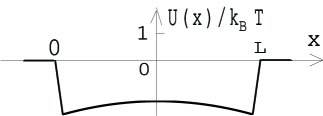
Figure 26: The electrostatic potential for cations across the channel with 5 dopants, considered in the text.

Unlike the $L$-dependent self-energy barrier considered above, the role of the Donnan potential is charge sensitive. In the negatively doped channel the Donnan potential well exists only for the cations while anions see the additional potential barrier. Thus, the Donnan potential naturally explains why in negatively doped biological channels the cation permeability is substantially larger than the anion one.

The contact potential $U_{D}$ may be augmented by the negative surface charge of the lipid membrane Appel or by affinity of internal walls to a selected ion, due to ion–specific short range interactions Doyle ; Hille . It seems that biological channels have evolved to compensate large electrostatic barrier by combined effect of $U_{D}$ and short range potentials. Our theory is helpful if one wants to study different components of the barrier or modify a channel. In narrow artificial nanopores there is no reason for compensation of electrostatic barrier. In this case, our theory may be verified by titration of wall charges.

X Conclusion

In this paper we studied the role of wall charges, which we call dopants, played in the charge transport through ion channels and nanopores. We considered various distributions of dopant charges and salt contents of the solution and showed that for all of them doping reduces the electrostatic self-energy barrier for ion transport. This conclusion is in qualitative agreement with general statement on the role of transitional binding inside the channel Bezrukov . In the simplest case of identical monovalent dopants and a monovalent salt solution such a reduction is monotonous and smooth function of the salt and dopant concentrations. The phenomenon is similar to the low-temperature Mott insulator-metal transition in doped semiconductors. However, due to the inefficiency of screening in one-dimensional geometry we arrived at a crossover rather than a transition even in infinite channel.

A remarkable observation of this paper is that the interplay of the ion entropy and the electrostatic energy may lead to true thermodynamic ion–exchange phase transitions. A necessary condition for such a transition to take place is the competition between more than one possible ground states. This in turn is possible for compensated (e.g. alternating) doping or for mixture of cations of various valency. The ion–exchange transitions are characterized by latent concentrations of ions. In other words, upon crossing a critical bulk concentration a certain amount of ions is suddenly absorbed or released by the channel. The phase transitions also lead to non-monotonic dependencies of the activation barrier as a function of the ion and dopant concentrations. For simplicity we restricted ourselves with the periodic arrangements of dopants. The existence of the phase transitions is a generic feature based only on the possibility of having more than one ground state with global charge neutrality. Thus they exist for arbitrary positioned dopants. In reality the phase transitions are smeared into relatively sharp crossovers due to finite size effects along with the finite electric field escape length, $\xi$.

We have also demonstrated that the doping can make the channels selective to one sign of monovalent salt ions or to divalent cations. This helps to understand how biological K, Na, Ca channels select cations and how Ca/Na channel selects Ca versus Na. The surprising fact is that Ca²⁺ ions, which could be expected to have four times larger self-energy barrier, actually exhibit the same barrier as Na⁺. This phenomenon is explained by fractionalization of Ca²⁺ on two unit-charge mobile solitons.

We study here only very simple models of a channel with charged walls. This is the price for many asymptotically exact results. Our results, of course, can not replace powerful numerical methods used for description of specific biological channels Roux .

In the future this theory may be used in nano-engineering projects such as modification of biological channels and design of long artificial nanopores. Another possible nano-engineering application deals with the transport of charged polymers through biological or artificial channels. A polymer moves slowly and for ions its charges may be considered as static. Therefore, for thin and stiff polymers in the channel, the charges on polymers can play the same role as doping. As a result, all the above discussions are directly applicable to the case of long charged polymer slowly moving through the channel. Changing the polymer one can change the dopants density.

In a more complicated scenario, the polymer can be bulky and occupy substantial part of the channel’s cross-section. Important example of such situation is translocation of a single stranded DNA molecule through the $\alpha$-Hemolysin channel Meller . In this case, the narrow part of the channel, immersed in the lipid membrane ($\beta$-barrel) can be approximated as an empty cylinder, while DNA may be considered as a coaxial cylinder blocking approximately a half of the channel cross-section. The dielectric constant of DNA is of the same order as one of lipids. Thus, the electric field lines of a charge located in the water gap between the two lipid cylinders are squeezed much stronger than in the empty channel. This may explain strong reduction of the ion current in presence of the DNA, which is also different for poly-A and poly-C DNA Meller . The latter remarkable observation inspires the hope that translocation of DNA may be used as a fast method of DNA sequencing. We shall discuss the bulky polymer situation in a future publication.

We are grateful to S. Bezrukov, A. I. Larkin and A. Parsegian for interesting discussions. A. K. is supported by the A.P. Sloan foundation and the NSF grant DMR–0405212. B. I. S was supported by NSF grant DMI-0210844.

Appendix A Phase transitions at large dopant concentration

In this appendix we discuss some details of the phase transitions at $\gamma_{c1}\approx 1.7$, $\gamma_{c2}\approx 5.3$, $\gamma_{c3}\approx 10.8$, etc, visible in Fig. 18. The free energy $F_{q}$ as function of the order parameter $q$ for a few values of $\gamma$ in the vicinity of $\gamma_{c1}$ is plotted in Fig. 27. The minimum, initially at $q=1/2$ for $\gamma_{c}<\gamma<\gamma_{c1}$, splits into two minima symmetrical around $1/2$. These two gradually move away from each other until they rich $q=0$ and $q=1$, correspondingly, for $\gamma>\gamma_{c1}$.

Figure 27: Free energy in units of $10^{-10}U_{L}(0)$ as a function of $q$ for $\gamma=1.7179330,~{}1.7179337,~{}1.7179341$ and $1.7179346$ (from top to bottom) with the same $\alpha_{2}=5\cdot 10^{-5}$. The graphs are vertically offset for clarity. The ground state continuously changes from $q=1/2$ to $q=0$.

The continuous variation of the absolute minimum (as opposed to the discrete a switch between the two fixed minima) suggests the second order phase transition scenario, taking place at $\gamma_{c1}$. The situation is more intricate, however. Namely, there are two (and not one) very closely spaced second order transitions, situated symmetrically around $\gamma_{c1}$ point. At the first transition the minima depart from $q=1/2$ and start moving towards $q=0$ and $q=1$, while at the second one they “stick” to $q=0,1$. Therefore, unless one has a very fine resolution (in $\gamma$ and/or $\alpha_{2}$), the entire behavior looks as a single first order transition.

The $F_{q}$ functions of Fig. 27 are very well fitted with the following phenomenological expression:

$$F_{q}(\gamma)=a(\gamma_{c1}-\gamma)\cos(2\pi q)+b\cos(4\pi q)\,,$$ (39)

where $a\gg b>0$. For any $\gamma$ the ground state corresponds to the value $q_{0}$ which minimizes $F_{q}$. Therefore $q_{0}$ is found from: either $\cos(2\pi q_{0})=(\gamma-\gamma_{c1}){a/(4b)}$, or $\sin(2\pi q_{0})=0$. The former equation has solutions only in the narrow interval $\gamma_{c1}-4b/a<\gamma<\gamma_{c1}+4b/a$. In this interval of dopant concentrations the minima move from $q=1/2$ to $q=0,1$. The edges of this interval constitute two second-order phase transitions located in the close proximity to each other. Near the first transition $|q_{0}-1/2|\simeq\sqrt{\gamma+4b/a-\gamma_{c1}}$, while near the second one: $|q_{0}|\simeq\sqrt{\gamma-4b/a-\gamma_{c1}}$. Therefore the critical exponent is the mean–field one: $\beta=1/2$. This could be anticipated for the system with the long-range interactions.

It is interesting to notice that the first order transition, discussed in the main text, may be also well fitted with Eq. (39) but with negative coefficients $a$ and $b$. The accuracy of our calculations is not sufficient to establish if the subsequent transitions are the first order ones or pairs of the very closely spaced second order transitions. As far as we can see the sequence of the reentrant transitions continues at larger dopant concentrations. Notice, however, that the difference of the corresponding free energies (and thus associated latent concentrations) are exponentially small at large $\gamma$.

References

- (1) B. Hille, Ion Channels of Excitable Membranes, Sinauer Associates, Sunderland, MA (2001).
- (2) D. A. Doyle et al., Science. 280, 69 (1998); R. MacKinnon, Nobel Lecture. Angew Chem Int Ed Engl 43 4265 (2004).
- (3) A. Parsegian, Nature 221, 844 (1969).
- (4) P. C. Jordan, Biophys J. 39, 157 (1982).
- (5) S. Teber, cond-mat/0501662.
- (6) A. Kamenev, J. Zhang, A. I. Larkin, B. I. Shklovskii, accpted to Physica A (2005); cond-mat/0503027.
- (7) J. Zhang, A. Kamenev, B. I. Shklovskii, Phys. Rev. Lett. 95, 148101 (2005).
- (8) J. Li, D. Stein, C. McMullan, D. Branton, M. J. Aziz, J. A. Golovchenko, Nature 412, 166 (2001); D. Stein, M. Kruithof, C. Dekker, Phys. Rev. Lett. 93, 035901 (2004); A. Aksimentiev, J. B. Heng, G. Timp, and K. Schulten, Biophys. J. 87, 2086 (2004); Z. Siwy, I. D. Kosinska, A. Fulinski, and C. R. Martin, Phys. Rev. Lett. 94, 048102 (2005).
- (9) The factor under the logarithm is the result of having two ions at every dopant, and factor of is obtained by integrating up the allowed volumes of the two ions for all possible ion configurations around the dopant.
- (10) W. Almers and E. W. McCleskey, J. Physiol. (Camb.) 353, 585 (1984).
- (11) S. F. Edwards and A. Lenard, J. Math. Phys. 3, 778 (1962).
- (12) A. Lenard, J. Math. Phys. 2, 682 (1961).
- (13) To prove it, consider the imaginary part of the Hamiltonian (25), , as a perturbation. Notice that this operator changes the parity of functions it acts on. The wave-functions of the unperturbed real Hermitian Hamiltonian are real and have a definite parity. It is clear then that only even–order (and thus purely real !) perturbative corrections to the spectrum can be non-zero. Moreover, since is anti–Hermitian, while is Hermitian, only even powers of contribute to this perturbation theory. As a result, the spectrum of the operator (25), , is a real symmetric function of .
- (14) H. J. Appel, E. Bamberg, H. Alpes, and P. Lauger, J. Membrane Biol. 31, 171 (1977).
- (15) W. R. Smythe, Static and Dynamic Electricity, 3-rd edition (chapter V), McGraw-Hill Book Company (1968). A. A. Kornyshev and M. A. Vorotyntsev, J. Phys. C: Solid State Phys. 12, 4939 (1979).
- (16) A. M. Berezhkovskii, M. A. Pustovoit, S. M. Bezrukov, J. Chem. Phys. 116, 6216, 9952 (2002); 119, 3943 (2003).
- (17) S. Kuyucak, O. S. Andersen, and S-H. Chung, Rep. Prog. Phys. 64, 1427 (2001); B. Nadler, U. Hollerbach, R. S. Eisenberg, Phys. Rev. E 68, 021905 (2003); B. Nadler, Z. Schuss, U. Hollerbach, R. S. Eisenberg, Phys. Rev. E 70, 051912 (2004); B. Roux, T. Allen, S. Berneche, W. Im, Quart. Rev. Biophys. 37, 15 (2004).
- (18) A. Meller, J. Phys. Cond. Matt. 15, R581 (2003).