Magnetic susceptibility of the body-centred orthorhombic La₂CuO₄ system

Abstract

A model Hamiltonian representing the Cu spins in La₂CuO₄ in its low-temperature body-centred orthorhombic phase, that includes both spin-orbit generated Dzyaloshinskii-Moriya interactions and interplanar exchange, is examined within the RPA utilizing a Tyablikov decoupling of various high-order Green’s functions. The magnetic susceptibility is evaluated as a function of temperature and the parameters quantifying these interactions, and compared to recently obtained experimental data of Lavrov, Ando and collaborators. An effective Hamiltonian corresponding to a simple tetragonal structure is shown to reproduce both the magnon spectra and the susceptibility of the more complicated body-centred orthorhombic model.

1 Introduction

Experimental studies of the magnetic and electronic properties of the cuprates continue to produce new and unexpected results that spur on theorists in their attempts to understand and describe the underlying orderings and excitations that may be involved in the pairing leading to high-temperature superconductivity. One experiment, that was the motivation for the work that we present in this paper, concerned the (zero-field) magnetic susceptibility of undoped La₂CuO₄ – it was found [1] that the magnetic response of undoped  La₂CuO₄ was highly anisotropic, and that this anisotropy persisted well above the Néel ordering temperature. Further, they found that this anisotropy persisted in the weakly doped state.

The importance of this result can be recognized if one notes the ongoing efforts of various researchers in understanding the origin and nature of so-called stripe correlations that are found in some cuprates (for a recent review of this problem, see reference [2]). That is, if the undoped state has a highly anisotropic magnetic susceptibility, can it really be that surprising that “spin stripes” are also present when the system is doped, and if not, what role does the anisotropic magnetic response play in the formation of stripe-like structures?

Previously, we have examined [3] the origin of this magnetic anisotropy by considering a single CuO₂ plane utilizing a magnetic Hamiltonian that contains spin-orbit generated Dzyaloshinskii-Moriya (DM) interactions [4, 5], and near-neighbour superexchange. If one includes both the symmetric and anti-symmetric DM interactions one finds that a true phase transition (at a non-zero temperature) occurs to an antiferromagnetic (AFM) state, wherein the AFM moment lies in the plane, with a weak parasitic ferromagnetic moment generated by a small canting of the moments out of the plane. Within mean-field theory, linear spin-wave theory, and within the RPA utilizing the Tyablikov decoupling scheme, we determined the magnetic susceptibility, and found (i) that it was indeed highly anisotropic, even when the DM interactions were small compared to near-neighbour intraplanar superexchange, and (ii) quantum fluctuations produced a substantial modification of the susceptibility as one used a more and more “sophisticated” theory [3]. Other potentially important terms (e.g., cyclic ring exchange [6]) that could have been included in that paper are discussed at the end of this paper.

In this report we focus on an augmented model that now includes the third dimension and the full body-centred orthorhombic structure of  La₂CuO₄. Our motivations for doing so are as the following. I – Although one can produce a true phase transition within a model that accounts for only a single plane, the interplanar exchange interactions can also produce a phase transition in approximately the same temperature range. That is, some researchers have suggested that both the (unfrustrated) interplanar exchange and the DM interactions are of comparable strength, and thus there is no good reason to exclude either of these terms in our model Hamiltonian (see [7] and references therein). II – As we discuss below, there are two different “near”-neighbour interplanar exchange constants, and these are different in different directions. Thus, this difference will be a source of magnetic anisotropy, and it is necessary to determine the extent of this anisotropy through a calculation that includes both the DM interactions and the interplanar exchange. III – As mentioned above, our previous work noted the strong effect of quantum fluctuations in a two-dimensional model. Since one expects such effects to be larger the lower the dimensionality of the system, it is possible that this behaviour is reduced in a full three-dimensional model. In this paper, again with the RPA utilizing the Tyablikov decoupling scheme, we have completed the requisite calculations for this more complicated but also more realistic magnetic Hamiltonian.

Our paper is organized as follows. In the next section we summarize the formalism necessary to analyze this problem; although somewhat similar formalism is presented our previous paper [3], when going from 2D to 3D the analysis is much more complicated, and it is thus necessary to present the required equations that must be solved. (Some aspects of the calculations have been put into various appendices.) In the subsequent section we present the results of a detailed and exhaustive numerical study of the resulting formalism for reasonable parameter values. Then we suggest a simpler model Hamiltonian, one for a simple tetragonal structure which avoids the frustrated interplanar AFM interactions of the original body-centred orthorhombic structure. Finally we conclude the paper by discussing the key results that we have obtained, and then provide a comparison between the predictions of our theory and the experiments of Lavrov, Ando and co-workers [1].

2 Model and Methods

2.1 Model Hamiltonian

We describe the magnetic structure of the La₂CuO₄ crystal in the low-temperature orthorhombic (LTO) phase by using an effective spin-$\frac{1}{2}$ Hamiltonian for the Cu²⁺ magnetic ions of the CuO₂ planes defined by

$$H = J\sum_{\langle i_{1},j_{1}\rangle}{\bf S}_{i_{1}}\cdot{\bf S}_{j_{1}}+\sum_{\langle i_{1},j_{1}\rangle}{\bf D}_{i_{1}j_{1}}\cdot({\bf S}_{i_{1}}\times{\bf S}_{j_{1}})+\sum_{\langle i_{1},j_{1}\rangle}{\bf S}_{i_{1}}\cdot\tilde{\Gamma}_{i_{1}j_{1}}\cdot{\bf S}_{j_{1}}$$ (1a)

$$+ J\sum_{\langle i_{2},j_{2}\rangle}{\bf S}_{i_{2}}\cdot{\bf S}_{j_{2}}+\sum_{\langle i_{2},j_{2}\rangle}{\bf D}_{i_{2}j_{2}}\cdot({\bf S}_{i_{2}}\times{\bf S}_{j_{2}})+\sum_{\langle i_{2},j_{2}\rangle}{\bf S}_{i_{2}}\cdot\tilde{\Gamma}_{i_{2}j_{2}}\cdot{\bf S}_{j_{2}}$$ (1b)

$$+ J_{\perp}\bigg{\{}\!\sum_{\langle i_{1},i_{2}\rangle}\!{\bf S}_{i_{1}}{\cdot}{\bf S}_{i_{2}}{+}\sum_{\langle j_{1},j_{2}\rangle}\!{\bf S}_{j_{1}}{\cdot}{\bf S}_{j_{2}}\!\bigg{\}}+J^{\prime}_{\perp}\bigg{\{}\!\sum_{\langle i_{1},j_{2}\rangle}\!{\bf S}_{i_{1}}{\cdot}{\bf S}_{j_{2}}{+}\sum_{\langle j_{1},i_{2}\rangle}\!{\bf S}_{j_{1}}{\cdot}{\bf S}_{i_{2}}\!\bigg{\}}~{}~{}.$$ (1c)

In this equation ${\bf S}_{i}$ denotes a spin at site $i$, and sites labelled as $i_{1}$ and $j_{1}$ are in the “first” plane while $i_{2}$ and $j_{2}$ are in the “second” (neighbouring) plane; the notation $\langle i_{\alpha},j_{\beta}\rangle$ refer to near-neighbour sites. This Hamiltonian is written within the $xyz$ orthorhombic coordinate system shown in figure 1 (see right-hand side) and in figure 2(a), in what we refer to as the “initial representation” in the LTO phase.

The various terms in the magnetic Hamiltonian given in equation (1) correspond to the following interactions. As was mentioned in the introduction, the orthorhombic distortion in the La₂CuO₄ crystal, together with the spin-orbit coupling, lead to the antisymmetric Dzyaloshinskii-Moriya ($\bf D$ term) and the symmetric pseudo-dipolar ($\tilde{\Gamma}$ term) interactions within the each CuO₂ plane [8, 9, 10]. These interactions together with superexchange one ($J$) can give rise to an ordered phase within a single CuO₂ plane at some nonzero temperature [3]. In this long-range ordered state Cu spins are aligned antiferromagnetically in the $y$-direction, with a small canting out of the plane. Therefore, each CuO₂ plane in a La₂CuO₄ crystal exhibits a net ferromagnetic moment, so-called weak ferromagnetism (WF) in the direction parallel to the $c$-axis of the Bmab space group ($z$-axis in the initial coordinates). Due to the weak antiferromagnetic coupling between the planes, the net ferromagnetic moments of adjacent CuO₂ planes are antiferromagnetically aligned and the system possesses no net moment.

Each Cu spin has four sites above and below it in neighbouring planes. If all of these distances were equal the system would be frustrated because the ordering in one plane would not lift the degeneracy that would result in adjacent planes. However, in the LTO phase these distances are not all equal, and thus the interplanar coupling between nearest-neighbour spins depends on which pair of neighbouring sites are considered. That is, due to the small orthorhombic distortion (relative to the high-temperature body-centred tetragonal phase) some near neighbour sites are closer together than other pairs (which are, technically, next-near-neighbour sites). In what follows we refer to the sites shown in figure 1, which allows for these ideas and the interplanar terms in equation (1c) to be made clear. The distance between $j_{1}$ and $j_{2}$ sites is slightly less than the distance between $j_{1}$ and $i_{2}$, and thus the superexchange couplings are different, and in this paper we thus specify that neighbouring spins in the $x-z$ plane ($J_{\perp}$ ) have a larger superexchange than do neighbouring spins in the $y-z$ plane ($J^{\prime}_{\perp}$): $|J_{\perp}|>|J^{\prime}_{\perp}|$ (see, for example, the discussion in reference [11]). As discussed in the introduction, and quantified in the next section, this difference immediately leads to an enhanced anisotropy of the magnetic susceptibility.

We schematically illustrate the magnetic structure of the La₂CuO₄ crystal within the ordered state ($T<T_{N}$) in figure 1, where arrows represent the Cu spin structure; this ordered state is quadripartite, as we now explain. In our notations we label sites in a plane with the spin canting up as $i_{1}$ and $j_{1}$, and correspondingly the sites of the nearest-neighbour planes with the spin canting down are labelled by indices $i_{2}$ and $j_{2}$. In each plane sites with label $i$ differ from the sites $j$ by the spin orientation within the antiferromagnetic order. Clearly, the magnetic structure of the La₂CuO₄ crystal in the ground state can be represented by four different sublattices with different spin orientations, and in our calculations we will follow the notation that $i_{1}$-sites belong to sublattice 1, $j_{1}$-sites to sublattice 2, $i_{2}$-sites to sublattice 3, and $j_{2}$-sites to sublattice 4. The interaction of the spins from the sublattice 1 and 2 with the nearest-neighbour spins from sublattice 3 and 4, respectively, are described by term $J_{\perp}$, and interaction with the spins from 4 and 3, respectively, are described by term $J^{\prime}_{\perp}$. Each magnetic ion interacts with the four nearest neighbour sites within its plane and with eight ions (four above and four below) from neighbouring planes.

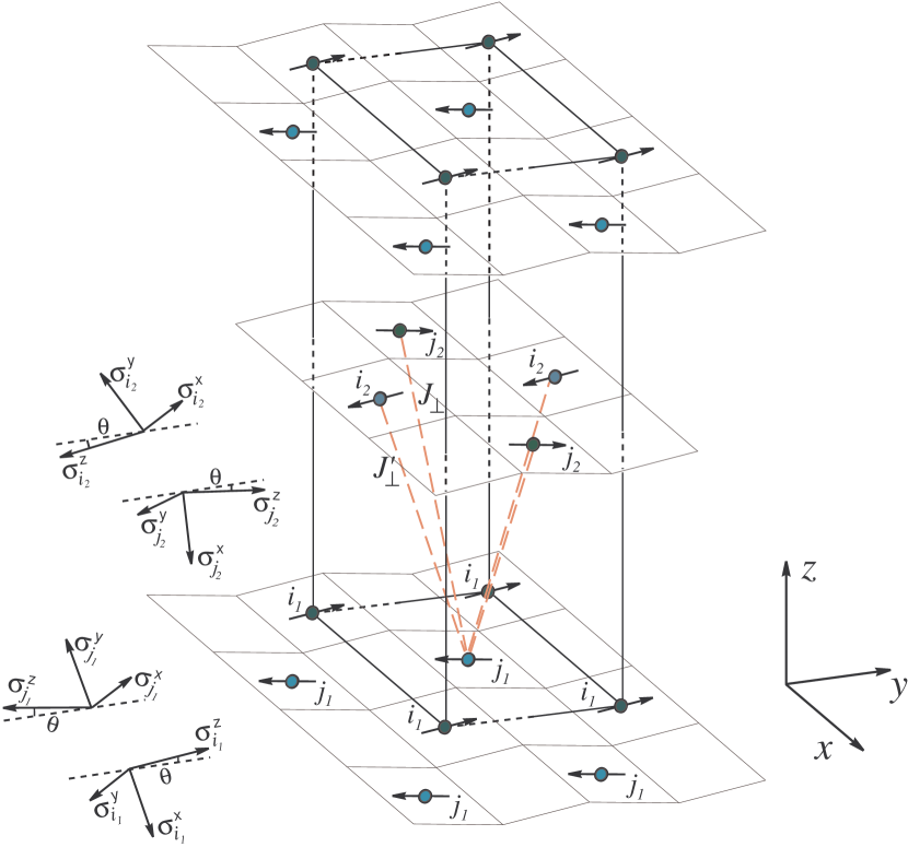
Figure 1: (Colour online) Magnetic structure of La₂CuO₄ crystal. Sites having different spin orientations are labelled by indices $i_{1}$, $j_{1}$ in the plane with the WF moment in the positive $z$ direction, and $i_{2}$, $j_{2}$ in the plane with the WF moment in the negative $z$ direction. For each set of sites the $\sigma$ spin coordinate system within the characteristic representation (CR) is shown. The thin net is shown only to simplify the visualization of the canting in the spin structure.

To summarize, the above presented magnetic Hamiltonian describes the magnetic interactions within the each CuO₂ plane in its first and second parts (equations (1a, 1b)), while the third part (equation (1c)) takes into account the weak interplanar superexchange couplings.

The structure of the Dzyaloshinskii-Moriya (DM) and the pseudo-dipolar interactions for the LTO phase are given by

$${\bf D}_{ab}=\frac{d}{\sqrt{2}}(-1,1,0),\qquad{\bf D}_{ac}=\frac{d}{\sqrt{2}}(-1,-1,0),$$ (1b)

and

$$\tilde{\Gamma}_{ab}=\left(\begin{array}[]{ccc}\Gamma_{1}&\Gamma_{2}&0\\ \Gamma_{2}&\Gamma_{1}&0\\ 0&0&\Gamma_{3}\end{array}\right),\qquad\tilde{\Gamma}_{ac}=\left(\begin{array}[]{ccc}\Gamma_{1}&-\Gamma_{2}&0\\ -\Gamma_{2}&\Gamma_{1}&0\\ 0&0&\Gamma_{3}\end{array}\right),$$ (1i)

within the initial coordinate system [3]. The DM vector given in equation (1b) alternates in sign on successive bonds in the $a-b$ and in the $a-c$ direction of each plane, as is represented schematically by the double arrows in figure 2(b).

(a)                                   (b)

Figure 2: (a) Coordinates in the initial representation. (b) Thin arrows — the Cu spins, and open arrows — the DM vectors.

Thin arrows in this figure describe the in-plane antiferromagnetic order of the Cu spins, and are canted up/down from the in-plane order by a small angle. In the classical ground state of the LTO phase the absolute value of the canting angles are equal on all sites and are given by the expression

$$\theta=\frac{1}{2}\tan^{-1}\Big{\{}\frac{d/\sqrt{2}}{J+\frac{1}{2}(\Gamma_{1}+\Gamma_{3})-\frac{1}{2}J^{\prime}_{\perp}}\Big{\}}.$$ (1j)

Following the scheme described in our earlier work [3], we perform rotations of the spin coordinate system in such a way that the new quantization axis ($\sigma^{z}$) is in the direction of a classical moment characterizing the ground state. Hereinafter we will call such a representation as the “characteristic representation” (CR). Since four different types of spin orientations are present in the magnetic structure of the La₂CuO₄ crystal, we introduce four different spin coordinate systems (see the left-hand side of figure 1) given by the transformations equations (1cl-1dp) in Appendix A. Thus, each sublattice consists its own spin coordinate system. The model Hamiltonian in terms of these spin operators $\sigma$ in the CR is given by

$$H_{\rm CR} = \sum_{\langle i_{1},j_{1}\rangle_{ab}}\left\{A(\sigma^{+}_{i_{1}}\sigma^{-}_{j_{1}}+\sigma^{-}_{i_{1}}\sigma^{+}_{j_{1}})-B^{*}\sigma^{+}_{i_{1}}\sigma^{+}_{j_{1}}-B\sigma^{-}_{i_{1}}\sigma^{-}_{j_{1}}-J_{2}\sigma^{z}_{i_{1}}\sigma^{z}_{j_{1}}\right\}$$

$$+ \sum_{\langle i_{1},j_{1}\rangle_{ac}}\left\{A(\sigma^{+}_{i_{1}}\sigma^{-}_{j_{1}}+\sigma^{-}_{i_{1}}\sigma^{+}_{j_{1}})+B\sigma^{+}_{i_{1}}\sigma^{+}_{j_{1}}+B^{*}\sigma^{-}_{i_{1}}\sigma^{-}_{j_{1}}-J_{2}\sigma^{z}_{i_{1}}\sigma^{z}_{j_{1}}\right\}$$

$$+ \sum_{\langle i_{2},j_{2}\rangle_{ab}}\left\{A(\sigma^{+}_{i_{2}}\sigma^{-}_{j_{2}}+\sigma^{-}_{i_{2}}\sigma^{+}_{j_{2}})+B\sigma^{+}_{i_{2}}\sigma^{+}_{j_{2}}+B^{*}\sigma^{-}_{i_{2}}\sigma^{-}_{j_{2}}-J_{2}\sigma^{z}_{i_{2}}\sigma^{z}_{j_{2}}\right\}$$

$$+ \sum_{\langle i_{2},j_{2}\rangle_{ac}}\left\{A(\sigma^{+}_{i_{2}}\sigma^{-}_{j_{2}}+\sigma^{-}_{i_{2}}\sigma^{+}_{j_{2}})-B^{*}\sigma^{+}_{i_{2}}\sigma^{+}_{j_{2}}-B\sigma^{-}_{i_{2}}\sigma^{-}_{j_{2}}-J_{2}\sigma^{z}_{i_{2}}\sigma^{z}_{j_{2}}\right\}$$

$$+ \!\!\sum_{\langle i_{1},j_{2}\rangle}\left\{\frac{1}{4}({J^{\prime}_{\perp}}{+}J_{p})(\sigma^{+}_{i_{1}}\sigma^{-}_{j_{2}}+\sigma^{-}_{i_{1}}\sigma^{+}_{j_{2}})+{\rm{i}}\frac{1}{4}({J^{\prime}_{\perp}}{-}J_{p})(\sigma^{+}_{i_{1}}\sigma^{+}_{j_{2}}-\sigma^{-}_{i_{1}}\sigma^{-}_{j_{2}})+J_{p}\sigma^{z}_{i_{1}}\sigma^{z}_{j_{2}}\right\}$$

$$+ \!\!\sum_{\langle j_{1},i_{2}\rangle}\left\{\frac{1}{4}({J^{\prime}_{\perp}}{+}J_{p})(\sigma^{+}_{j_{1}}\sigma^{-}_{i_{2}}+\sigma^{-}_{j_{1}}\sigma^{+}_{i_{2}})+{\rm{i}}\frac{1}{4}({J^{\prime}_{\perp}}{-}J_{p})(\sigma^{+}_{j_{1}}\sigma^{+}_{i_{2}}-\sigma^{-}_{j_{1}}\sigma^{-}_{i_{2}})+J_{p}\sigma^{z}_{j_{1}}\sigma^{z}_{i_{2}}\right\}$$

$$+ J_{\perp}\!\!\sum_{\langle i_{1},i_{2}\rangle}\left\{\frac{\rm{i}}{2}(\sigma^{+}_{i_{1}}\sigma^{+}_{i_{2}}{-}\sigma^{-}_{i_{1}}\sigma^{-}_{i_{2}}){-}\sigma^{z}_{i_{1}}\sigma^{z}_{i_{2}}\right\}+J_{\perp}\!\!\sum_{\langle j_{1},j_{2}\rangle}\left\{\frac{\rm{i}}{2}(\sigma^{+}_{j_{1}}\sigma^{+}_{j_{2}}{-}\sigma^{-}_{j_{1}}\sigma^{-}_{j_{2}}){-}\sigma^{z}_{j_{1}}\sigma^{z}_{j_{2}}\right\},$$

where we have used the following definitions:

$$A=\frac{J_{1}-J_{3}}{4},\qquad B=\frac{J_{4}}{2}+{\rm i}\frac{J_{1}+J_{3}}{4},$$ (1o)

$$J_{1}=J+\Gamma_{1},\qquad J_{p}=J^{\prime}_{\perp}\cos 2\theta,$$

$$J_{2}=\hphantom{-}\frac{\Gamma_{1}{-}\Gamma_{3}}{2}+\left(J+\frac{\Gamma_{1}{+}\Gamma_{3}}{2}\right)\cos 2\theta+\frac{d}{\sqrt{2}}\sin 2\theta,$$

$$J_{3}=-\frac{\Gamma_{1}{-}\Gamma_{3}}{2}+\left(J+\frac{\Gamma_{1}{+}\Gamma_{3}}{2}\right)\cos 2\theta+\frac{d}{\sqrt{2}}\sin 2\theta,$$

$$J_{4}=-\Gamma_{2}\sin\theta+\frac{d}{\sqrt{2}}\cos\theta.$$ (1p)

The subscripts $\langle i,j\rangle_{ab}$ and $\langle i,j\rangle_{ac}$ in the summations of equation (2.1) imply the nearest neighbours in the $ab$ and $ac$ directions, respectively, as shown in figure 2(b).

2.2 Mean field analysis

In this subsection, we present the results of the mean field approximation (MFA) for the above Hamiltonian by following the standard decoupling. That is, in the MFA in equation (1) we use

$$\sigma_{i}^{a}\sigma_{j}^{b}\rightarrow\langle\sigma_{i}^{a}\rangle~{}\sigma_{j}^{b}~{}+~{}\sigma_{i}^{a}~{}\langle\sigma_{j}^{b}\rangle~{}-~{}\langle\sigma_{i}^{a}\rangle~{}\langle\sigma_{j}^{b}\rangle,$$ (1q)

where $a$ and $b$ can be equal to any of $x,y,z$. Then, the equation for the order parameter, to be denoted by $\eta$, within the MFA reads as

$$\eta\equiv\langle\sigma^{z}\rangle=\frac{1}{2}\tanh\left\{\frac{\beta}{2}{\cal Z}[J_{2}+J_{\perp}-J_{p}]\langle\sigma^{z}\rangle\right\},$$ (1r)

where ${\cal Z}=4$ is the in-plane coordination number, and $\beta=1/T$. From this equation the Néel temperature at which $\eta$ vanishes can be written immediately as

$$T^{MFA}_{N}=J_{2}+J_{\perp}-J_{p}~{}~{}.$$ (1s)

By applying a magnetic field sequentially in the $x$, $y$, and $z$ directions of each coordinate systems within the CR we can find the transverse and longitudinal components of susceptibility within all four sublattices. Using the relation between the components of susceptibility in the initial and characteristic representations given in equations (1dr-1dt), we obtain the final result for the zero-field uniform susceptibility within the MFA below the ordering temperature ($T<T^{MFA}_{N}$)

$$\chi^{x~{}MFA} = \frac{1}{4}\frac{1}{J_{1}{+}J_{2}{+}2J_{\perp}{+}(J^{\prime}_{\perp}{-}J_{p})},$$ (1t)

$$\chi^{y~{}MFA} = \frac{1}{4}\frac{\sin^{2}(\theta)}{J_{2}{-}J_{3}{+}2J_{\perp}{-}2J_{p}}+\frac{\cos^{2}\theta}{4}\frac{{\rm{sech}}^{2}\left\{\frac{\beta}{2}{\cal Z}\eta J_{mfa}\right\}}{T+[J_{2}{+}J_{\perp}{+}J_{p}]\>{\rm{sech}}^{2}\left\{\frac{\beta}{2}{\cal Z}\eta J_{mfa}\right\}},$$ (1u)

$$\chi^{z~{}MFA} = \frac{1}{4}\frac{\cos^{2}(\theta)}{J_{2}{+}J_{3}{+}2J_{\perp}}+\frac{\sin^{2}\theta}{4}\frac{{\rm{sech}}^{2}\left\{\frac{\beta}{2}{\cal Z}\eta J_{mfa}\right\}}{T-[J_{2}{-}J_{\perp}{+}J_{p}]\>{\rm{sech}}^{2}\left\{\frac{\beta}{2}{\cal Z}\eta J_{mfa}\right\}},$$ (1v)

where we define

$$J_{mfa}=J_{2}+J_{\perp}-J_{p}~{}~{},$$ (1w)

and the equation for the order parameter $\eta$ given by equation (1r). We used the “mfa” subscript in equation (1w) because this combination determines the effective interaction, and thus the Néel temperature within the mean field theory (see equation (1r)).

The final results for the components of the susceptibility in the initial representation for high temperatures, that is above the ordering temperature ($T>T^{MFA}_{N}$), are

$$\chi^{x~{}MFA} = \frac{1}{4}\frac{1}{T+J_{1}+J_{\perp}+J^{\prime}_{\perp}},$$ (1x)

$$\chi^{y~{}MFA} = \frac{1}{4}\frac{\sin^{2}(\theta)}{T-J_{3}+J_{\perp}-J_{p}}+\frac{1}{4}\frac{\cos^{2}(\theta)}{T+J_{2}+J_{\perp}+J_{p}},$$ (1y)

$$\chi^{z~{}MFA} = \frac{1}{4}\frac{\cos^{2}(\theta)}{T+J_{3}+J_{\perp}+J_{p}}+\frac{1}{4}\frac{\sin^{2}(\theta)}{T-J_{2}+J_{\perp}-J_{p}}.$$ (1z)

In the limit $T\to T^{MFA}_{\rm N}$ we obtain that the $x$ component of the susceptibility is continuous at the transition and is given by equation (1t). The $y$ component of the susceptibility at the transition temperature reads

$$\chi^{y~{}MFA}\bigg{|}_{T\to T^{MFA}_{\rm N}}=\frac{1}{4}\frac{\sin^{2}(\theta)}{J_{2}-J_{3}+2J_{\perp}-2J_{p}}+\frac{\cos^{2}\theta}{8}\frac{1}{J_{\perp}+J_{2}}.$$ (1aa)

Note that with respect to the pure 2D case [3] the $z$ component of the susceptibility does not diverge at the Néel point and also is continuous at the transition

$$\chi^{z~{}MFA}\bigg{|}_{T\to T^{MFA}_{\rm N}}=\frac{1}{4}\frac{\cos^{2}(\theta)}{J_{2}+J_{3}+2J_{\perp}}+\frac{1}{8}\frac{\sin^{2}(\theta)}{J_{\perp}-J_{p}}.$$ (1ab)

2.3 Random phase approximation

In this part of the paper we use the technique of the double-time temperature dependent Green’s functions within the framework of the random-phase approximation (RPA). In the imaginary-time formalism, the temperature dependent Green’s function and the corresponding equation of motion for two Bose-type operators reads

$$G_{AB}(\tau)=\langle T_{\tau}A(\tau)B(0)\rangle,\quad\frac{{\rm d}G_{AB}(\tau)}{{\rm d}\tau}=\delta(\tau)\langle[A,B]\rangle+\langle T_{\tau}[H(\tau),A(\tau)]B(0)\rangle,$$ (1ac)

where $A(\tau)={\rm e}^{H\tau}A{\rm e}^{-H\tau}$ is the operator in the Heisenberg representation for imaginary time argument $\tau$, and $T_{\tau}$ is the time-ordering operator.

By using the method proposed originally by Liu [12], we employ the perturbed Hamiltonian

$$H^{f}_{1}=H_{\rm CR}-f\sum_{i^{\prime}_{1}}\sigma^{z}_{i^{\prime}_{1}},\qquad i^{\prime}_{1}\in\mbox{ sublattice 1}$$ (1ad)

to find the longitudinal components of the susceptibility in the CR. In the equation (1ad) $f$ is a small fictitious field applied to the spins of sublattice 1 only. In this paper we are studying the zero-field uniform magnetic susceptibility, therefore we restrict $f$ to be constant and static.

The Green’s functions to be used in present calculations are

$$G^{f}_{i_{1}j_{1}}(\tau)=\langle T_{\tau}\sigma^{+}_{i_{1}}(\tau)\sigma^{-}_{j_{1}}(0)\rangle^{f},\quad G^{f-}_{i_{1}j_{1}}(\tau)=\langle T_{\tau}\sigma^{-}_{i_{1}}(\tau)\sigma^{-}_{j_{1}}(0)\rangle^{f},$$

$$G^{f}_{j^{\prime}_{1}j_{1}}(\tau)=\langle T_{\tau}\sigma^{+}_{j^{\prime}_{1}}(\tau)\sigma^{-}_{j_{1}}(0)\rangle^{f},\quad G^{f-}_{j^{\prime}_{1}j_{1}}(\tau)=\langle T_{\tau}\sigma^{-}_{j^{\prime}_{1}}(\tau)\sigma^{-}_{j_{1}}(0)\rangle^{f},$$ (1ae)

$$G^{f}_{i_{2}j_{1}}(\tau)=\langle T_{\tau}\sigma^{+}_{i_{2}}(\tau)\sigma^{-}_{j_{1}}(0)\rangle^{f},\quad G^{f-}_{i_{2}j_{1}}(\tau)=\langle T_{\tau}\sigma^{-}_{i_{2}}(\tau)\sigma^{-}_{j_{1}}(0)\rangle^{f},$$

$$G^{f}_{j^{\prime}_{2}j_{1}}(\tau)=\langle T_{\tau}\sigma^{+}_{j^{\prime}_{2}}(\tau)\sigma^{-}_{j_{1}}(0)\rangle^{f},\quad G^{f-}_{j^{\prime}_{2}j_{1}}(\tau)=\langle T_{\tau}\sigma^{-}_{j^{\prime}_{2}}(\tau)\sigma^{-}_{j_{1}}(0)\rangle^{f},$$

where $\langle...\rangle^{f}$ means that all expectation values are taken with respect to the perturbed Hamiltonian in equation (1ad). After an expansion in a power series of $f$ the Green’s function, e.g. $G^{f}_{i_{1}j_{1}}(\tau)$, reads

$$G^{f}_{i_{1}j_{1}}(\tau)=G^{(0)}_{i_{1}j_{1}}(\tau)+fG^{(1)}_{i_{1}j_{1}}(\tau)+O(f^{2}).$$ (1af)

Since $G^{(0)}_{i_{1}j_{1}}(\tau)=G_{i_{1}j_{1}}(\tau)$, from now we drop the superscript and use

$$G^{f}_{i_{1}j_{1}}(\tau)=G_{i_{1}j_{1}}(\tau)+fG^{(1)}_{i_{1}j_{1}}(\tau)+O(f^{2}).$$ (1ag)

Also, we introduce

$$\langle\sigma^{z}_{i_{1}}(\tau)\rangle^{f}=\langle\sigma^{z}_{i_{1}}\rangle+f{\rm v}_{i_{1}}+O(f^{2}),$$ (1ah)

where, due to the translation periodicity $\langle\sigma^{z}_{i_{1}}\rangle=\eta$, the order parameter at $f=0$.

Now let us find the equation of motion for the Green’s function $G^{f}_{i_{1}j_{1}}(\tau)$. The equations for other functions can be found in the same way. Starting from the equation (1ac) we can write

$$\frac{{\rm d}G^{f}_{i_{1}j_{1}}(\tau)}{{\rm d}\tau}=2\delta(\tau)\delta_{i_{1}j_{1}}\langle\sigma^{z}_{i_{1}}\rangle^{f}+\langle T_{\tau}[H_{\rm CR}(\tau),\sigma^{+}_{i_{1}}(\tau)]\sigma^{-}_{j_{1}}(0)\rangle^{f}-fG^{f}_{i_{1}j_{1}}.$$ (1ai)

In order to solve this equation of motion we are following the RPA scheme, and using the so-called Tyablikov’s decoupling [13] which is given by

$$\langle T_{\tau}\sigma^{z}_{l}(\tau)\sigma^{+}_{i_{1}}(\tau)\sigma^{-}_{j_{1}}(0)\rangle^{f}\to\langle\sigma^{z}_{l}(\tau)\rangle^{f}\langle T_{\tau}\sigma^{+}_{i_{1}}(\tau)\sigma^{-}_{j_{1}}(0)\rangle^{f}=\langle\sigma^{z}_{l}(\tau)\rangle^{f}G^{f}_{i_{1}j_{1}}(\tau).$$ (1aj)

After this decoupling is introduced, equation (1ai) is found to be

$$\frac{{\rm d}G^{f}_{i_{1}j_{1}}(\tau)}{{\rm d}\tau} = 2\delta(\tau)\delta_{i_{1}j_{1}}\langle\sigma^{z}_{i_{1}}\rangle^{f}-fG^{f}_{i_{1}j_{1}}(\tau)$$

$$-\!\!\sum_{\delta_{ab}}\left\{\!2\langle\sigma^{z}_{i_{1}}(\tau)\rangle^{f}[AG^{f}_{(i_{1}{+}\delta)j_{1}}(\tau)-BG^{f-}_{(i_{1}{+}\delta)j_{1}}(\tau)]+J_{2}\langle\sigma^{z}_{i_{1}{+}\delta}(\tau)\rangle^{f}G^{f}_{i_{1}j_{1}}(\tau)\!\right\}$$

$$-\!\!\sum_{\delta_{ac}}\left\{2\langle\sigma^{z}_{i_{1}}(\tau)\rangle^{f}[AG^{f}_{(i_{1}{+}\delta)j_{1}}(\tau){+}B^{*}G^{f-}_{(i_{1}{+}\delta)j_{1}}(\tau)]+J_{2}\langle\sigma^{z}_{i_{1}{+}\delta}(\tau)\rangle^{f}G^{f}_{i_{1}j_{1}}(\tau)\right\}$$

$$-\!\!\sum_{\langle j^{\prime}_{2}\rangle_{i_{1}}}\left\{2\langle\sigma^{z}_{i_{1}}(\tau)\rangle^{f}\bigg{[}\frac{J^{\prime}_{\perp}{+}J_{p}}{4}G^{f}_{j^{\prime}_{2}j_{1}}(\tau)-{\rm{i}}\frac{J^{\prime}_{\perp}{-}J_{p}}{4}G^{f-}_{j^{\prime}_{2}j_{1}}(\tau)\bigg{]}-J_{p}\langle\sigma^{z}_{j^{\prime}_{2}}(\tau)\rangle^{f}G^{f}_{i_{1}j_{1}}(\tau)\!\right\}$$

$$-\!\!\sum_{\langle i^{\prime}_{2}\rangle_{i_{1}}}\left\{-{\rm{i}}J_{\perp}\langle\sigma^{z}_{i_{1}}(\tau)\rangle^{f}G^{f-}_{i^{\prime}_{2}j_{1}}(\tau)+J_{\perp}\langle\sigma^{z}_{i^{\prime}_{2}}(\tau)\rangle^{f}G^{f}_{i_{1}j_{1}}(\tau)\!\right\},$$

where $\sum_{\delta_{ab}}$ refers to a summation over the nearest neighbours of the sites $i_{1}$ in the $ab$ direction of the same CuO₂ plane, and similarly for $\sum_{\delta_{ac}}$ — see figure 2(b). Thus, in equation (2.3) all sites $i_{1}+\delta$ belong to the sublattice 2. The notation $\sum_{\langle i^{\prime}_{2}\rangle_{i_{1}}}$ means sum over all sites $i^{\prime}_{2}$ from sublattice 3 which are nearest neighbours of sites $i_{1}$ that belong to the sublattice 1, and similarly for $\sum_{\langle j^{\prime}_{2}\rangle_{i_{1}}}$.

Next, we perform the transformation into the momentum-frequency representation for the Green’s functions and the spin operators:

$$G^{f}_{i_{1}j_{1}}(\tau) = \frac{4}{N\beta}\sum_{\boldsymbol{k},m}G^{f}_{12}(\boldsymbol{k},\omega_{m}){\rm e}^{{\rm i}\boldsymbol{k}\cdot({\bf R}_{i_{1}}-{\bf R}_{j_{1}})}{\rm e}^{-{\rm i}\omega_{m}\tau},$$ (1al)

$$\langle\sigma^{z}_{i_{1}}(\tau)\rangle^{f} = \frac{1}{\beta}\sum_{\boldsymbol{k},m}\langle\sigma^{z}_{1}(\boldsymbol{k},\omega_{m})\rangle^{f}{\rm e}^{-{\rm i}\boldsymbol{k}\cdot{\bf R}_{i_{1}}}{\rm e}^{-{\rm i}\omega_{m}\tau}=\sum_{\boldsymbol{k}}\delta(\boldsymbol{k})[\eta+f{\rm v}_{1}]{\rm e}^{-{\rm i}\boldsymbol{k}\cdot{\bf R}_{i_{1}}},$$ (1am)

where the expansion of equation (1ah) and the linear response to the uniform perturbation expressed by ${\rm v}_{1}(\boldsymbol{k})=\delta(\boldsymbol{k}){\rm v}_{1}$ were taken into account. In the transformation given by equations (1al, 1am), the sum over $\boldsymbol{k}$ runs over $\frac{1}{4}N$ points of the first Brillouin zone, and $\omega_{n}=2\pi n/\beta$ for $n\in\mathbb{Z}$ are the Bose Matsubara frequencies. The equation of motion for the Green’s function $G^{f}_{i_{1}j_{1}}(\tau)$ in the momentum-frequency representation reads

$$-{\rm i}\omega_{m}G^{f}_{12}(\boldsymbol{k},\omega_{m}) = -2{\cal Z}A_{\boldsymbol{k}}[\eta+f{\rm v}_{1}]G^{f}_{22}(\boldsymbol{k},\omega_{m})+2{\cal Z}B_{\boldsymbol{k}}[\eta+f{\rm v}_{1}]G^{f-}_{22}(\boldsymbol{k},\omega_{m})$$

$$-2{\cal Z}\>a_{\boldsymbol{k}}[\eta+f{\rm v}_{1}]G^{f}_{42}(\boldsymbol{k},\omega_{m})+2{\cal Z}\>{\rm{i}}b_{\boldsymbol{k}}[\eta+f{\rm v}_{1}]G^{f-}_{42}(\boldsymbol{k},\omega_{m})$$

$$+2{\cal Z}\>{\rm{i}}d_{\boldsymbol{k}}[\eta+f{\rm v}_{1}]G^{f-}_{32}(\boldsymbol{k},\omega_{m})-fG^{f}_{12}(\boldsymbol{k},\omega_{m})$$

$$-{\cal Z}\bigg{\{}J_{2}[\eta+f{\rm v}_{2}]+J_{\perp}[\eta+f{\rm v}_{3}]-J_{p}[\eta+f{\rm v}_{4}]\bigg{\}}G^{f}_{12}(\boldsymbol{k},\omega_{m}),$$

where, as before, ${\cal Z}$ is the in-plane coordination number, and we introduce

$$A_{\boldsymbol{k}}=A\gamma_{\boldsymbol{k}},\quad B_{\boldsymbol{k}}=(\Re B)\gamma_{\boldsymbol{k}}^{\prime}+{\rm{i}}(\Im B)\gamma_{\boldsymbol{k}},$$ (1ao)

$$a_{\boldsymbol{k}}=\frac{J^{\prime}_{\perp}+J_{p}}{4}\xi_{\boldsymbol{k}},\quad b_{\boldsymbol{k}}=\frac{J^{\prime}_{\perp}-J_{p}}{4}\xi_{\boldsymbol{k}},\quad d_{\boldsymbol{k}}=\frac{J_{\perp}}{2}\xi^{\prime}_{\boldsymbol{k}},$$ (1ap)

$$\gamma_{\boldsymbol{k}}=\frac{1}{2}(\cos k_{x}+\cos k_{y}),\quad\xi_{\boldsymbol{k}}=\cos k_{z}\cos\bigg{(}\frac{k_{x}+k_{y}}{2}\bigg{)},$$ (1aq)

$$\gamma^{\prime}_{\boldsymbol{k}}=\frac{1}{2}(\cos k_{x}-\cos k_{y}),\quad\xi^{\prime}_{\boldsymbol{k}}=\cos k_{z}\cos\bigg{(}\frac{k_{x}-k_{y}}{2}\bigg{)}.$$ (1ar)

Now we can write down the final equations for the zero-order in $f$ Green’s function $G_{12}(\boldsymbol{k},\omega_{m})$, and the first-order one $G^{(1)}_{12}(\boldsymbol{k},\omega_{m})$

$$\frac{{\rm i}\omega_{m}}{2{\cal Z}\eta}G_{12} = \bigg{\{}\frac{J_{2}}{2}{+}\frac{J_{\perp}}{2}{-}\frac{J_{p}}{2}\bigg{\}}G_{12}+A_{\boldsymbol{k}}G_{22}-B_{\boldsymbol{k}}G^{-}_{22}+a_{\boldsymbol{k}}G_{42}-{\rm{i}}b_{\boldsymbol{k}}G^{-}_{42}-{\rm{i}}d_{\boldsymbol{k}}G^{-}_{32},$$ (1as)

$$\frac{{\rm i}\omega_{m}}{2{\cal Z}\eta}G^{(1)}_{12} = \frac{G_{12}}{2{\cal Z}\eta}+\bigg{\{}\frac{J_{2}}{2}\frac{{\rm{v}}_{2}}{\eta}{+}\frac{J_{\perp}}{2}\frac{{\rm{v}}_{3}}{\eta}{-}\frac{J_{p}}{2}\frac{{\rm{v}}_{4}}{\eta}\bigg{\}}G_{12}+\frac{{\rm{v}}_{1}}{\eta}\bigg{(}\frac{{\rm{i}}\omega}{2{\cal Z}\eta}-\bigg{\{}\frac{J_{2}}{2}{+}\frac{J_{\perp}}{2}{-}\frac{J_{p}}{2}\bigg{\}}\bigg{)}G_{12}$$

$$+ \bigg{\{}\frac{J_{2}}{2}{+}\frac{J_{\perp}}{2}{-}\frac{J_{p}}{2}\bigg{\}}G^{(1)}_{12}+A_{\boldsymbol{k}}G^{(1)}_{22}-B_{\boldsymbol{k}}G^{(1)-}_{22}+a_{\boldsymbol{k}}G^{(1)}_{42}-{\rm{i}}b_{\boldsymbol{k}}G^{(1)-}_{42}-{\rm{i}}d_{\boldsymbol{k}}G^{(1)-}_{32}$$

where in these equations we drop the wave vector and frequency dependencies for the Green’s functions; that is $G=G(\boldsymbol{k},\omega_{m})$ and $G^{(1)}=G^{(1)}(\boldsymbol{k},\omega_{m})$.

In order to obtain a closed set of the equations for the zero and first order Green’s function we should use the above described scheme for the all other functions in equation (1ae), and the final system of equations for the zero and first-order Green’s function are given in the Appendix B in equations (1du-1dw). The structure of the system for the zero-order functions is identical with the system of equations for the first-order ones, except for the free terms. Hence, the poles of the zero-order Green’s functions (that determine the spectrum of the spin-wave excitations) $G(\boldsymbol{k},\omega_{m})$ are equal to the poles for the first-order ones $G^{(1)}(\boldsymbol{k},\omega_{m})$, and are found to be

$$\varepsilon_{1,\boldsymbol{k}}=2{\cal Z}\eta\omega_{1,\boldsymbol{k}}=\sqrt{\alpha_{1,\boldsymbol{k}}+\sqrt{\beta_{1,\boldsymbol{k}}}}~{}~{},\qquad\varepsilon_{2,\boldsymbol{k}}=2{\cal Z}\eta\omega_{2,\boldsymbol{k}}=\sqrt{\alpha_{1,\boldsymbol{k}}-\sqrt{\beta_{1,\boldsymbol{k}}}}~{}~{},$$ (1au)

$$\varepsilon_{3,\boldsymbol{k}}=2{\cal Z}\eta\omega_{3,\boldsymbol{k}}=\sqrt{\alpha_{2,\boldsymbol{k}}+\sqrt{\beta_{2,\boldsymbol{k}}}}~{}~{},\qquad\varepsilon_{4,\boldsymbol{k}}=2{\cal Z}\eta\omega_{4,\boldsymbol{k}}=\sqrt{\alpha_{2,\boldsymbol{k}}-\sqrt{\beta_{2,\boldsymbol{k}}}}~{}~{},$$

$$\alpha_{1,\boldsymbol{k}}=a_{\boldsymbol{k}}^{2}+(A_{\boldsymbol{k}}{-}J_{mfa}/2)^{2}-(b_{\boldsymbol{k}}{-}d_{\boldsymbol{k}})^{2}-|B_{\boldsymbol{k}}|^{2},$$ (1av)

$$\alpha_{2,\boldsymbol{k}}=a_{\boldsymbol{k}}^{2}+(A_{\boldsymbol{k}}{+}J_{mfa}/2)^{2}-(b_{\boldsymbol{k}}{+}d_{\boldsymbol{k}})^{2}-|B_{\boldsymbol{k}}|^{2},$$

$$\beta_{1,\boldsymbol{k}}=4[a_{\boldsymbol{k}}(A_{\boldsymbol{k}}{-}J_{mfa}/2)-(b_{\boldsymbol{k}}{-}d_{\boldsymbol{k}})\Im B_{\boldsymbol{k}}]^{2}-(2\Re B_{\boldsymbol{k}})^{2}[a_{\boldsymbol{k}}^{2}-(b_{\boldsymbol{k}}{-}d_{\boldsymbol{k}})^{2}],$$ (1aw)

$$\beta_{2,\boldsymbol{k}}=4[a_{\boldsymbol{k}}(A_{\boldsymbol{k}}{+}J_{mfa}/2)-(b_{\boldsymbol{k}}{+}d_{\boldsymbol{k}})\Im B_{\boldsymbol{k}}]^{2}-(2\Re B_{\boldsymbol{k}})^{2}[a_{\boldsymbol{k}}^{2}-(b_{\boldsymbol{k}}{+}d_{\boldsymbol{k}})^{2}],$$

within the notation of equations (1ao, 1ap), and the MFA-inspired definition of $J_{mfa}=J_{2}+J_{\perp}-J_{p}$.

The free terms in the first-order systems (see equation (1dw)) are determined by the zero-order Green’s functions, and thus the first-order quantities $G^{(1)}$ can be written down in terms of the solution for the zero-order system C, and the as-yet-unknown quantities ${\rm v}_{1}$, ${\rm v}_{2}$, ${\rm v}_{3}$, and ${\rm v}_{4}$.

To calculate ${\rm v}_{1,2,3,4}$ we use a relation that connects ${\rm v}$ and the Green’s functions $G^{(1)}(\boldsymbol{k},\tau=0^{-})$, viz.

$$-{\rm v}_{l} = \frac{4}{N}\sum_{\boldsymbol{k}}G^{(1)}_{ll}(\boldsymbol{k},0^{-}),\qquad l=1,2,3,4.$$ (1ax)

After the substitution of the solutions of the systems of equations for the first-order Green’s functions $G^{(1)}(\boldsymbol{k},\omega_{m})$ in D into the system of equations for ${\rm v}_{l}$ in equation (1ax), the results are found to be

$${\rm{v}}_{1}-{\rm{v}}_{2}-{\rm{v}}_{3}+{\rm{v}}_{4}=\frac{\frac{1}{\beta}\sum\limits_{m}{\rm{e}}^{-{\rm{i}}\omega_{m}0^{-}}{\cal N}^{y}(\omega_{m})}{2\eta-\frac{1}{\beta}\sum\limits_{m}{\rm{e}}^{-{\rm{i}}\omega_{m}0^{-}}\left\{{\rm{i}}\omega_{m}{\cal D}^{y}(\omega_{m})/\eta-2{\cal Z}(J_{\perp}{+}J_{2}){\cal N}^{y}(\omega_{m})\right\}},$$ (1ay)

$${\rm{v}}_{1}+{\rm{v}}_{2}-{\rm{v}}_{3}-{\rm{v}}_{4}=\frac{\frac{1}{\beta}\sum\limits_{m}{\rm{e}}^{-{\rm{i}}\omega_{m}0^{-}}{\cal N}^{z}(\omega_{m})}{2\eta-\frac{1}{\beta}\sum\limits_{m}{\rm{e}}^{-{\rm{i}}\omega_{m}0^{-}}\left\{{\rm{i}}\omega_{m}{\cal D}^{z}(\omega_{m})/\eta-2{\cal Z}(J_{\perp}{-}J_{p}){\cal N}^{z}(\omega_{m})\right\}},$$ (1az)

where

$${\cal N}^{y}(\omega_{m})=\frac{4}{N}\sum_{\boldsymbol{k}}\bigg{\{}|G_{22}|^{2}{-}|G_{12}|^{2}{+}|G^{-}_{22}|^{2}{-}|G^{-}_{12}|^{2}{-}|G_{42}|^{2}{+}|G_{32}|^{2}{-}|G^{-}_{42}|^{2}{+}|G^{-}_{32}|^{2}\bigg{\}}~{}~{},$$

$${\cal D}^{y}(\omega_{m})=\frac{4}{N}\sum_{\boldsymbol{k}}\bigg{\{}|G_{22}|^{2}{-}|G_{12}|^{2}{-}|G^{-}_{22}|^{2}{+}|G^{-}_{12}|^{2}{-}|G_{42}|^{2}{+}|G_{32}|^{2}{+}|G^{-}_{42}|^{2}{-}|G^{-}_{32}|^{2}\bigg{\}}~{}~{},$$

(1ba)

$${\cal N}^{z}(\omega_{m})=\frac{4}{N}\sum_{\boldsymbol{k}}\bigg{\{}|G_{22}|^{2}{+}|G_{12}|^{2}{+}|G^{-}_{22}|^{2}{+}|G^{-}_{12}|^{2}{-}|G_{42}|^{2}{-}|G_{32}|^{2}{-}|G^{-}_{42}|^{2}{-}|G^{-}_{32}|^{2}\bigg{\}}~{}~{},$$

$${\cal D}^{z}(\omega_{m})=\frac{4}{N}\sum_{\boldsymbol{k}}\bigg{\{}|G_{22}|^{2}{+}|G_{12}|^{2}{-}|G^{-}_{22}|^{2}{-}|G^{-}_{12}|^{2}{-}|G_{42}|^{2}{-}|G_{32}|^{2}{+}|G^{-}_{42}|^{2}{+}|G^{-}_{32}|^{2}\bigg{\}}~{}~{},$$

and all zero-order Green’s functions $G(\boldsymbol{k},\omega_{m})$ are given in C.

Now let us find the quantities which determine the linear response to a magnetic field applied to the one of sublattices (e.g., see equation (1dq)). The longitudinal $z$ components of the susceptibility in the characteristic representation are given by

$$\chi^{\sigma^{z}\sigma^{z}}_{11}=\frac{\partial\langle\sigma^{z}_{1}\rangle^{f}}{\partial f}\Big{|}_{f=0}={\rm v}_{1},\qquad\chi^{\sigma^{z}\sigma^{z}}_{12}=\frac{\partial\langle\sigma^{z}_{2}\rangle^{f}}{\partial f}\Big{|}_{f=0}={\rm v}_{2},$$ (1bc)

$$\chi^{\sigma^{z}\sigma^{z}}_{13}=\frac{\partial\langle\sigma^{z}_{3}\rangle^{f}}{\partial f}\Big{|}_{f=0}={\rm v}_{3},\qquad\chi^{\sigma^{z}\sigma^{z}}_{14}=\frac{\partial\langle\sigma^{z}_{4}\rangle^{f}}{\partial f}\Big{|}_{f=0}={\rm v}_{4},$$

where the expansion of equation (1ah) was used. The transverse $x$ and $y$ components of the susceptibility tensor are determined in the terms of Green’s functions to be given by

$$\chi^{\sigma^{\alpha}\sigma^{\alpha^{\prime}}}_{11}\!\!=\frac{4}{N}\sum_{i_{1},i^{\prime}_{1}}\int^{\beta}_{0}\!\!\langle T_{\tau}\sigma_{i_{1}}^{\alpha}(\tau)\sigma_{i^{\prime}_{1}}^{\alpha^{\prime}}(0)\rangle{\rm d}\tau,\quad\chi^{\sigma^{\alpha}\sigma^{\alpha^{\prime}}}_{12}\!\!=\frac{4}{N}\sum_{i_{1},j_{1}}\int^{\beta}_{0}\!\!\langle T_{\tau}\sigma_{i_{1}}^{\alpha}(\tau)\sigma_{j_{1}}^{\alpha^{\prime}}(0)\rangle{\rm d}\tau,$$ (1bd)

$$\chi^{\sigma^{\alpha}\sigma^{\alpha^{\prime}}}_{13}\!\!=\frac{4}{N}\sum_{i_{1},i^{\prime}_{2}}\int^{\beta}_{0}\!\!\langle T_{\tau}\sigma_{i_{1}}^{\alpha}(\tau)\sigma_{i^{\prime}_{2}}^{\alpha^{\prime}}(0)\rangle{\rm d}\tau,\quad\chi^{\sigma^{\alpha}\sigma^{\alpha^{\prime}}}_{14}\!\!=\frac{4}{N}\sum_{i_{1},j_{2}}\int^{\beta}_{0}\!\!\langle T_{\tau}\sigma_{i_{1}}^{\alpha}(\tau)\sigma_{j_{2}}^{\alpha^{\prime}}(0)\rangle{\rm d}\tau,$$

where $\alpha=x,y$. By substituting the solutions in C into the definition in equation (1bd) for the transverse components of susceptibility, we obtain the result given in E. This result for the transverse components in the CR is exactly the same as the MFA calculations for the transverse components.

Then, using equations (1dr)-(1dt) the components of the susceptibility in the initial coordinate system of equation (1) below the transition temperature are found to be

$$\chi^{x} = \frac{1}{4}\frac{1}{J_{1}{+}J_{2}{+}2J_{\perp}{+}(J^{\prime}_{\perp}{-}J_{p})},$$ (1be)

$$\chi^{y} = \frac{1}{4}\frac{\sin^{2}(\theta)}{J_{2}{-}J_{3}{+}2J_{\perp}{-}2J_{p}}+\cos^{2}(\theta)[{\rm v}_{1}-{\rm v}_{2}-{\rm v}_{3}+{\rm v}_{4}],$$ (1bf)

$$\chi^{z} = \frac{1}{4}\frac{\cos^{2}(\theta)}{J_{2}{+}J_{3}{+}2J_{\perp}}+\sin^{2}(\theta)[{\rm v}_{1}+{\rm v}_{2}-{\rm v}_{3}-{\rm v}_{4}]~{}~{}.$$ (1bg)

These expressions for the components of susceptibility include the as-yet-unknown value of the order parameter $\eta$. It can be found directly; from the definition of the Green’s functions we have

$$G_{nn}(\tau=0^{-})=\langle\sigma^{-}_{n}\sigma^{+}_{n}\rangle=\frac{1}{2}-\eta,\quad G_{nn}(\tau=0^{-})=\frac{2}{N}\sum_{\boldsymbol{k}}G_{22}(\boldsymbol{k},\tau=0^{-}).$$ (1bh)

Substituting $G_{22}(\boldsymbol{k},\omega)$ from equation (C), and performing the summation on the Matsubara frequencies, the equation for the order parameter turns out to be

$$\frac{1}{\eta}=\frac{1}{2}\frac{4}{N}\sum_{\boldsymbol{k}}\bigg{\{}\!\! \bigg{(}y_{1,\boldsymbol{k}}{+}\frac{x_{1,\boldsymbol{k}}}{\sqrt{\beta_{1,\boldsymbol{k}}}}\bigg{)}\frac{2n(\varepsilon_{1,\boldsymbol{k}}){+}1}{\omega_{1,\boldsymbol{k}}}+\bigg{(}y_{1,\boldsymbol{k}}{-}\frac{x_{1,\boldsymbol{k}}}{\sqrt{\beta_{1,\boldsymbol{k}}}}\bigg{)}\frac{2n(\varepsilon_{2,\boldsymbol{k}}){+}1}{\omega_{2,\boldsymbol{k}}}$$

$$+ \bigg{(}y_{2,\boldsymbol{k}}{+}\frac{x_{2,\boldsymbol{k}}}{\sqrt{\beta_{2,\boldsymbol{k}}}}\bigg{)}\frac{2n(\varepsilon_{3,\boldsymbol{k}}){+}1}{\omega_{3,\boldsymbol{k}}}+\bigg{(}y_{2,\boldsymbol{k}}{-}\frac{x_{2,\boldsymbol{k}}}{\sqrt{\beta_{2,\boldsymbol{k}}}}\bigg{)}\frac{2n(\varepsilon_{4,\boldsymbol{k}}){+}1}{\omega_{4,\boldsymbol{k}}}\bigg{\}}~{}~{},$$

where

$$x_{1,\boldsymbol{k}} = -2a_{\boldsymbol{k}}[a_{\boldsymbol{k}}(A_{\boldsymbol{k}}{-}J_{mfa}/2)-(b_{\boldsymbol{k}}{-}d_{\boldsymbol{k}})\Im B_{\boldsymbol{k}}],\qquad y_{1,\boldsymbol{k}}=-(A_{\boldsymbol{k}}{-}J_{mfa}/2),$$

$$x_{2,\boldsymbol{k}} = \hphantom{-}2a_{\boldsymbol{k}}[a_{\boldsymbol{k}}(A_{\boldsymbol{k}}{+}J_{mfa}/2)-(b_{\boldsymbol{k}}{+}d_{\boldsymbol{k}})\Im B_{\boldsymbol{k}}],\qquad y_{2,\boldsymbol{k}}=\hphantom{-}(A_{\boldsymbol{k}}{+}J_{mfa}/2),$$

$$n(\varepsilon_{l,\boldsymbol{k}}) = [\exp(\beta\varepsilon_{l,\boldsymbol{k}})-1]^{-1},\qquad l=1,2,3,4.$$

Since the order parameter (viz., the sublattice magnetization) is temperature dependent, it follows that the spectrum of elementary excitations (equation (1au)) is also temperature dependent.

The Néel temperature at which $\eta$ vanishes within the adopted RPA approximation is determined by

$$T_{\rm N}=\bigg{[}\frac{1}{2{\cal Z}}\frac{4}{N}\sum_{\boldsymbol{k}}\bigg{\{}\!\! \bigg{(}y_{1,\boldsymbol{k}}{+}\frac{x_{1,\boldsymbol{k}}}{\sqrt{\beta_{1,\boldsymbol{k}}}}\bigg{)}\frac{1}{\omega^{2}_{1,\boldsymbol{k}}}+\bigg{(}y_{1,\boldsymbol{k}}{-}\frac{x_{1,\boldsymbol{k}}}{\sqrt{\beta_{1,\boldsymbol{k}}}}\bigg{)}\frac{1}{\omega^{2}_{2,\boldsymbol{k}}}$$

$$+ \bigg{(}y_{2,\boldsymbol{k}}{+}\frac{x_{2,\boldsymbol{k}}}{\sqrt{\beta_{2,\boldsymbol{k}}}}\bigg{)}\frac{1}{\omega^{2}_{3,\boldsymbol{k}}}+\bigg{(}y_{2,\boldsymbol{k}}{-}\frac{x_{2,\boldsymbol{k}}}{\sqrt{\beta_{2,\boldsymbol{k}}}}\bigg{)}\frac{1}{\omega^{2}_{4,\boldsymbol{k}}}\bigg{\}}\bigg{]}^{-1}.$$

By putting $\eta\to 0$ we find that the $z$-component of the susceptibility $\chi^{z}$ in equation (1bg) does not diverges at the Néel temperature, whereas it diverges for the pure 2D model ($J_{\perp}=J_{\perp}^{\prime}=0$). At the Néel temperature all components of the susceptibility within the RPA are equal to the MFA results, the latter of which are given in equations (1t, 1aa, 1ab).

For completeness, we mention that the investigation of the model equation (1) within linear spin-wave (LSW) theory leads to the same structure of the susceptibility expressions as we found within the RPA in equations (1be-1bg). The main difference between the results in RPA and LSW theory comes from the calculation of the longitudinal components of the susceptibility in the CR. The spin-wave theory gives unity in the denominator of the expressions in equations (1ay, 1az), and $S=1/2$ instead of the order parameter $\eta$ everywhere in the numerator ${\cal N}^{y}$ and ${\cal N}^{z}$. The transverse components of the susceptibility in the CR are equal within the all of the MFA, RPA, and SW theories.

When the temperature of the system is above the Néel temperature, $T_{N}$, there still exists short-range antiferromagnetic order. To model such an order we follow reference [12] and introduce a fictitious field $h$ pointing in the direction of the sublattice magnetization, that is the $z$ direction in the characteristic representation. To this end, the Hamiltonian

$$H_{h}=H_{\rm CR}-h\sum_{i}\sigma^{z}_{i}-h\sum_{j}\sigma^{z}_{j}$$ (1bk)

is used, and the limit $h\to 0$ is taken after the calculation is carried out.

Above the Néel temperature, we define a (different) order parameter by

$${\cal Y}=\lim_{h\to 0}(2{\cal Z}\eta/h).$$ (1bl)

By a procedure similar to the above presented [3] (that is, the RPA scheme below $T_{N}$) we have found the equation for the order parameter and all components of the magnetic susceptibility in the paramagnetic phase. It is then possible to show that paramagnetic version of the equation for the order parameter in equation (2.3) leads to

$$\beta=\frac{1}{2{\cal Z}}\frac{4}{N}\sum_{\boldsymbol{k}}\bigg{\{}\!\! \bigg{(}y_{1,\boldsymbol{k}}{+}\frac{x_{1,\boldsymbol{k}}}{\sqrt{\beta_{1,\boldsymbol{k}}}}\bigg{)}\frac{1}{\omega^{2}_{1,\boldsymbol{k}}}+\bigg{(}y_{1,\boldsymbol{k}}{-}\frac{x_{1,\boldsymbol{k}}}{\sqrt{\beta_{1,\boldsymbol{k}}}}\bigg{)}\frac{1}{\omega^{2}_{2,\boldsymbol{k}}}$$

$$+ \bigg{(}y_{2,\boldsymbol{k}}{+}\frac{x_{2,\boldsymbol{k}}}{\sqrt{\beta_{2,\boldsymbol{k}}}}\bigg{)}\frac{1}{\omega^{2}_{3,\boldsymbol{k}}}+\bigg{(}y_{2,\boldsymbol{k}}{-}\frac{x_{2,\boldsymbol{k}}}{\sqrt{\beta_{2,\boldsymbol{k}}}}\bigg{)}\frac{1}{\omega^{2}_{4,\boldsymbol{k}}}\bigg{\}}.$$

where in all expressions for $x_{1,2}$, $y_{1,2}$, $\beta_{1,2}$ and $\omega_{1-4}$ which determine equation (2.3) in the paramagnetic phase, we use a new definition for $J_{mfa}$ (which we now call $\tilde{J}_{mfa}$) that reads

$$\tilde{J}_{mfa}=J_{2}+J_{\perp}-J_{p}+\frac{1}{\cal Y}.$$ (1bn)

The quantity ${\cal Y}$ approaches infinity as the temperature is lowered to $T_{\rm N}$. Indeed, putting ${\cal Y}\to\infty$ in equation (2.3) we find the temperature at which ${\cal Y}$ diverges, which is identically equal to the Néel temperature.

We have found (see below for numerical results) that for model equation (1) all components of susceptibility are continuous at the Néel point within the RPA.

3 Numerical Results

In this section we present the result of numerical calculations of the system modelled by the Hamiltonian of equation (1) based on the above-presented analytical formulae.

3.1 Parameters regimes

Firstly, let us consider the set of model parameters that appears in the Hamiltonian of equation (1), viz. in-plane parameters $J$, $d$ and $\Gamma$, and out-of-plane parameters $J_{\perp}$ and $J^{\prime}_{\perp}$. The in-plane parameter $d$ that describes the antisymmetric DM interaction and parameters $\Gamma_{1,2,3}$ that give the pseudo-dipolar anisotropy, are of order $10^{-2}$ and $10^{-4}$ respectively in units of $J$ [9, 10], and it has been shown that the only combination from the pseudo-dipolar terms that affects the behaviour of the system is $\Delta\Gamma\equiv\Gamma_{1}-\Gamma_{3}$ [3, 14]. Thus, the in-plane part of the model, that is equations (1a,1b), can be completely described by the AFM Heisenberg model with the DM antisymmetric exchange interaction ${\bf D}$ and XY-like pseudo-dipolar anisotropy given by $\Delta\Gamma$.

In order to examine the behaviour of the system with respect to the out-of-plane parameters, we introduce the combination

$$\Delta J_{\perp}{\equiv}J_{\perp}-J^{\prime}_{\perp}~{}~{},$$ (1bo)

that describes the interplanar anisotropy interaction between nearest-neighbour spins which we refer to as the net interplanar coupling, and the combination

$$\tilde{J}_{\perp}{\equiv}J_{\perp}{+}J^{\prime}_{\perp}~{}.$$ (1bp)

In our calculations we take $\Delta J_{\perp}$ to be of the order $10^{-5}-10^{-4}$ in units of $J$ (see [7] and references therein).

In this subsection we focus on the behaviour of order parameter $\eta$, Néel temperature $T_{\rm N}$, and susceptibility $\chi$ with respect to the parameter $\tilde{J}_{\perp}$ within the RPA method (we present a detailed consideration of the dependence on $\Delta J_{\perp}$ in a subsequent subsection). Firstly, we find that the order parameter and the Néel temperature are almost independent of the $\tilde{J}_{\perp}$ within a wide range of the model parameters. In figure 3 we show two representative plots for the order parameter and the susceptibility for certain values of the in-plane parameters. In each line of the figure 3a (that is solid, dotted, and dashed lines) we have simultaneously plotted five data sets, each with different values of the parameter $\tilde{J}_{\perp}$ that has been varied from zero up to $0.5J$ ($\tilde{J}_{\perp}/J=0,0.01,0.1,0.2,0.5$). As one can see, for such a wide range of the parameter $\tilde{J}_{\perp}$ there is virtually no difference of the absolute values of the Néel temperature and the order parameter, whereas the relatively small changes of the net interplanar coupling $\Delta J_{\perp}$ in figure 3a strongly affects these quantities.

Figure 3: (Colour online) The (a) order parameter vs. $T/J$ for the different values of $\Delta J_{\perp}$: $\Delta J_{\perp}{=}0$ – black solid line, $\Delta J_{\perp}{=}0.1{\times}10^{-3}J$ – blue dotted line, $\Delta J_{\perp}{=}0.4{\times}10^{-3}J$ – red dashed line, and each line consists of five data sets with $\tilde{J}_{\perp}$ varying from zero up to $0.5J$. The (b) susceptibility, in units of $1/J$, vs. $T/T_{N}$ for $\Delta J_{\perp}{=}0$, and for the following values of $\tilde{J}_{\perp}$: $\tilde{J}_{\perp}{=}0$ up to $0.02$ — upper plot (many curves are superimposed on top of one another), $\tilde{J}_{\perp}{=}0.2$ — middle plot, and $\tilde{J}_{\perp}{=}0.5$ — lower plot. In both figures (a) and (b) we have fixed $d/J=0.02$ and $\Delta\Gamma/J=0.42\times 10^{-3}$.

In case of the susceptibility, its dependence on $\tilde{J}_{\perp}$ differs from that discussed above for the order parameter $\eta$. Now, as is seen in figure 3b, the parameter $\tilde{J}_{\perp}$ generates the constant shift in the $\chi^{x}$ and $\chi^{z}$ components of susceptibility as well as the constant shift in the $\chi^{y}$ near the Néel temperature and within the paramagnetic region. However, for the reasonable values of the out-of-plane model parameters (that is $J_{\perp},\;J^{\prime}_{\perp}<10^{-3}J$) the parameter $\tilde{J}_{\perp}$ does not affect on the behaviour of the susceptibility with temperature.

This latter result for the susceptibility can be shown in various limits from the above analytical results by taking into account the small magnitude of $\Delta J_{\perp}$ and the in-plane parameters $d$ and $\Delta\Gamma$ with respect to $J$. In the zero temperature limit one can write down the susceptibility in the following form:

$$\chi^{x,z}_{T\to 0}\approx\frac{1}{4}\frac{1}{2J+\tilde{J}_{\perp}},\quad\chi^{y}_{T\to 0}\approx\frac{1}{32}\frac{1}{\{J-\tilde{J}_{\perp}/4\}^{2}}\frac{d^{2}}{\Delta\Gamma+2\Delta J_{\perp}}.$$ (1bq)

Also, near the Néel temperature one finds

$$\chi^{y}_{T\to T_{\rm N}} \approx \frac{1}{32}\frac{1}{\{J-\tilde{J}_{\perp}/4\}^{2}}\frac{d^{2}}{\Delta\Gamma+2\Delta J_{\perp}}+\frac{1}{4}\frac{1}{2J+\tilde{J}_{\perp}},$$ (1br)

$$\chi^{z}_{T\to T_{\rm N}} \approx \frac{1}{4}\frac{1}{2J+\tilde{J}_{\perp}}+\frac{1}{8}\frac{1}{\tilde{J}_{\perp}}.$$ (1bs)

Almost everywhere within the above presented equations (1bq-1bs) one can ignore the contribution of $\tilde{J}_{\perp}<10^{-3}J$ with respect to $J$; only the $z$-component of the susceptibility $\chi^{z}$ at the Néel temperature is strongly affected by $\tilde{J}_{\perp}$, as shown in equation (1bs). In fact, the upper plot in figure 3b consists of data sets with the different values of the parameter $\tilde{J}_{\perp}$ over the range of zero up to $0.02J$, but these differing plots can not be distinguished from one another.

Similarly, the parameter $\tilde{J}_{\perp}$ can be ignored in the expressions for the spin-wave gaps, as can be clearly seen from the following approximate formulae

$$\omega_{1,\boldsymbol{k}\to 0}^{2} \approx \bigg{\{}J-\frac{\tilde{J}_{\perp}}{2}\bigg{\}}\bigg{(}\Delta J_{\perp}+\frac{d}{\sqrt{2}}\theta-\big{\{}J-\frac{\tilde{J}_{\perp}}{2}\big{\}}\theta^{2}\bigg{)},$$ (1bt)

$$\omega_{2,\boldsymbol{k}\to 0}^{2} \approx \bigg{\{}J+\frac{\tilde{J}_{\perp}}{2}\bigg{\}}\bigg{(}\frac{d}{\sqrt{2}}\theta-\big{\{}J-\frac{\tilde{J}_{\perp}}{2}\big{\}}\theta^{2}\bigg{)},$$ (1bu)

$$\omega_{3,\boldsymbol{k}\to 0}^{2} \approx \bigg{\{}J-\frac{\tilde{J}_{\perp}}{2}\bigg{\}}(\Delta\Gamma/2+\Delta J_{\perp}),$$ (1bv)

$$\omega_{4,\boldsymbol{k}\to 0}^{2} \approx \bigg{\{}J+\frac{\tilde{J}_{\perp}}{2}\bigg{\}}\Delta\Gamma/2.$$ (1bw)

Therefore, one can conclude that the affect of the parameter $\tilde{J}_{\perp}$ on the physics of the model is negligibly small. Consequently, without further trepidations the system can be studied using a fixed and representative value of this parameter, e.g. $\tilde{J}_{\perp}=10^{-3}J$, without having to be concerned with it changing our results.

At the end of this subsection we discuss briefly the case of isotropic interplanar coupling ($\Delta J_{\perp}=0$). In such a case the only difference in the susceptibility, with respect to a pure 2D model [3], is the finite value of $\chi^{z}$ at the Néel temperature. Then, only the in-plane anisotropies are responsible for the anisotropic magnetic properties of such a system, viz. the behaviour of susceptibility, order parameter, and spin-wave excitations. We emphasize the perhaps expected result, that for the 3D case with isotropic interplanar coupling, due to the frustration of interplanar coupling within the body-centred lattice, the effects of 2D quantum fluctuations and short-range correlations are very important, whereas the interplanar coupling is not.

3.2 Néel temperature and spin-wave excitations

Now we present the results of our numerical investigations of the Néel temperature and the spin wave excitations and their dependence on the parameters of the in-plane anisotropies $d/J$, $\Delta\Gamma/J$, and the out-of plane anisotropy $\Delta J_{\perp}/J$.

Figure 4a shows the Néel temperature obtained within the RPA scheme as a function of both $\Delta\Gamma/J$ and $\Delta J_{\perp}/J$. We found that the transition temperature $T_{N}$ depends on both the in-plane XY-like pseudo-dipolar anisotropy parameter $\Delta\Gamma$ and the out-of-plane anisotropy parameter $\Delta J_{\perp}$, and changes of the same order ($\sim 10^{-4}J$) in $\Delta J_{\perp}$ and/or in $\Delta\Gamma$ produces considerable changes in the Néel temperature, $T_{N}$. Further, the dependence of the Néel temperature on the DM parameter is shown in figure 4b: $T_{N}$ decreases as $d$ increases for small $d$, but for larger values of the DM interaction, i.e. $d\gg\Delta J_{\perp},\Delta\Gamma$, the Néel temperature $T_{N}$ increases nearly linearly with $d$. The transition temperature into the long-range ordered state, $T_{N}$, increases as the parameter $\Delta J_{\perp}$ increases since the net interplanar coupling that each spin feels favours to the AFM state.

Figure 4: (Colour online) The Néel temperature $T_{N}$, in units of $J$, vs. (a) $\Delta J_{\perp}/J$ – black solid line (fixed $\Delta\Gamma/J=0.42\times 10^{-3}$) and $\Delta\Gamma/J$ – blue dotted line (fixed $\Delta J_{\perp}/J=0.42\times 10^{-3}$), both for fixed $d/J=0.02$, as well as vs. (b) the DM parameter $d/J$ (fixed $\Delta\Gamma/J=0.42\times 10^{-3}$ and $\Delta J_{\perp}/J=0.42\times 10^{-3}$).

Figure 5 shows the zero-temperature energy gaps in the long wavelength limit as a function of in- and out- of plane anisotropy parameters, and the resulting behaviours can be understood immediately from equations (1bt)-(1bw). Two modes, $\varepsilon_{1}$ and $\varepsilon_{2}$, are almost independent of $\Delta\Gamma$ (see figure 5a, and equations (1bt,1bu)), but they show a strong dependency on the DM parameter, $d$, as seen in figure 5b. Since the canted angle goes as $\theta\approx(d/\sqrt{2})/(2J)$, the modes $\varepsilon_{1}$, $\varepsilon_{2}$ are nearly linear in $d$. In the limit of zero DM interaction the mode $\varepsilon_{2}$ goes to zero and a Goldstone mode appears in the spin-wave spectrum, while the mode $\varepsilon_{1}$ goes to a finite value, which is about $2{\cal Z}\eta\sqrt{J\Delta J_{\perp}}$ (see equations (1bt,1bu)). Two other modes in the spectrum, $\varepsilon_{3}$, $\varepsilon_{4}$, are almost independent of the DM parameter of anisotropy, while they vary strongly with $\Delta\Gamma$. In the limit $\Delta\Gamma=0$ the mode $\varepsilon_{4}$ goes to zero and another Goldstone mode appears in the spectrum, while the mode $\varepsilon_{3}$ goes to the finite value of about $2{\cal Z}\eta\sqrt{J\Delta\Gamma/2}$ (equation (1bv,1bw)). Since in the case of 3D model thermal fluctuations do not destroy the long-range ordering for $T\neq 0$, the Néel temperature does not go to zero when a Goldstone mode $\varepsilon_{2}$ or $\varepsilon_{4}$ appears in the spectrum.

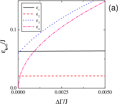
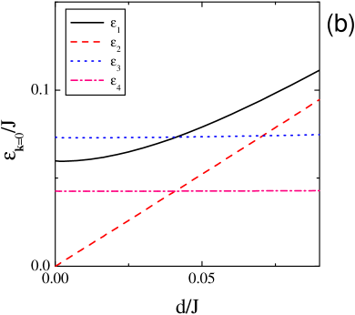
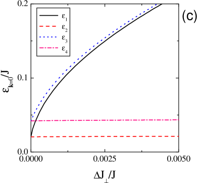
Figure 5: (Colour online) The energy gaps, in units of $J$, as function of
(a) XY-like anisotropy parameter $\Delta\Gamma/J$ ($d/J=0.02$, $\Delta J_{\perp}/J=0.42\times 10^{-3}$),
(b) DM parameter $d/J$ ($\Delta\Gamma/J=0.42\times 10^{-3}$, $\Delta J_{\perp}/J=0.42\times 10^{-3}$), and
(c) out-of-plane anisotropy parameter $\Delta J_{\perp}/J$ ($d/J=0.02$, $\Delta\Gamma/J=0.42\times 10^{-3}$).

Lastly, we note that the plots of figure 5c show that two modes ($\varepsilon_{2}$ and $\varepsilon_{4}$) are independent of the net interplanar coupling $\Delta J_{\perp}$, and two modes ($\varepsilon_{1}$ and $\varepsilon_{3}$) demonstrate a square-root dependency on $\Delta J_{\perp}$. When the net interplanar coupling goes to zero, $\Delta J_{\perp}=0$, the two modes $\varepsilon_{1}$ and $\varepsilon_{2}$ become equal and describe the in-plane mode in the spin-wave excitations [15]. Similarly, the mode $\varepsilon_{3}$ coincides with $\varepsilon_{4}$ at $\Delta J_{\perp}=0$ and they correspond to the out-of-plane magnon mode [15].

3.3 Susceptibility

Now we consider the temperature behaviour of the susceptibility and examine its dependency on different values of the in-plane and out-of plane anisotropy parameters. Our results for the $y$, and $z$ components of the susceptibility within the different approximation schemes, viz. RPA, LSW theory, and MFA, are presented in figure 6 ($T<T_{N}$). We do not present the similar comparing for the $x$ component of susceptibility because of the pure transverse component $\chi^{x}$ (see equation (1be)) has the same value within all mentioned approximations (below the transition temperature). On the other hand, the longitudinal (in the characteristic representation equations  (1ds,1dt)) components of the susceptibility are involved in the equations for the components $\chi^{y}$ and $\chi^{z}$ that leads to their different temperature behaviours within the different approximation methods (see below).

Our results for the $y$ component of the susceptibility, $\chi^{y}$, are shown in figure 6a. We find that at low temperatures the RPA analytical scheme, as was also found in pure 2D case [3], is in good agreement with the linear spin-wave theory. Plots in figure 6a also show that RPA results agree with the MFA as one nears the transition temperature $T_{N}$, and both RPA and MFA lead to the same magnitude of susceptibility at the Néel temperature. (It is worth noting here that transition temperature $T_{N}$ within the MFA approach, where $T_{N}=J_{2}+J_{\perp}-J_{p}\approx J$, is almost independent of the anisotropy, in contrast to the RPA scheme where $T_{N}$ is very sensitive to the anisotropy parameters (see figure 4).) One can also see that in the zero temperature limit all approximations used in the paper go to the same value of susceptibility approximately given by equation (1bq).

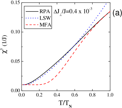
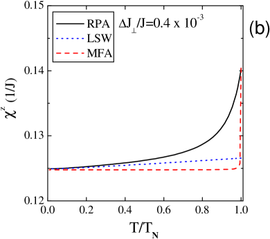
Figure 6: (Colour online) The (a) $\chi^{y}$ and (b) $\chi^{z}$ components of the susceptibility, in units of $1/J$ – a comparison of the RPA (black solid line), LSW (blue dotted line) and MFA (red dashed line) results below $T_{N}$ (for $d/J=0.02$, $\Delta\Gamma/J=0.42\times 10^{-3}$, $\Delta J_{\perp}/J=0.4\times 10^{-3}$).

Figure 6b shows the $z$ component of the susceptibility $\chi^{z}$, and again we obtain the good agreement between the RPA and LSW methods at low $T$, and coincidence of all results in the zero temperature limit. On the other hand, in the vicinity of the transition temperature, the RPA scheme gives qualitatively different behaviour of $\chi^{z}$ with respect to the MFA and LSW formalisms. Thus, we can answer one of the motivating questions of this study: Does the extension of the model of reference [3] from 2D to 3D lead to a reduction of the strong effects of quantum fluctuations? Indeed, the answer is no, and there are strong effects of quantum fluctuations in our 3D Heisenberg model with the anisotropies. This statement is correct for a magnitude of the net interplanar coupling $\Delta J_{\perp}$ up to $\sim 10^{-3}J$.

Now let us find the correlation between the ratio of spin-waves modes of the magnon excitation spectrum in the long wavelength limit, and the behaviour of the components of susceptibility in the zero temperature limit (similar to the correlation that we have found in the pure 2D model [3]). Firstly, from the analytical results, equation (1bq), we obtain that the ratio between the components of the susceptibility is given approximately by

$$\frac{\chi^{y}}{\chi^{x,z}}\bigg{|}_{T\to 0}\approx\frac{d^{2}}{4J(\Delta\Gamma+2\Delta J_{\perp})}.$$ (1bx)

Next, by taking into account that the canted angle is $\theta\approx(d/\sqrt{2})/(2J)$ and $\tilde{J}_{\perp}\ll J$, we can rewrite the expressions (1bt)-(1bw) that specify the spin-wave gaps, which we write in a scaled form using $\varepsilon_{l}=2{\cal Z}\eta\omega_{l}$ as

$$\omega_{1}^{2}\approx J\Delta J_{\perp}+d^{2}/8,\quad\omega_{2}^{2}\approx d^{2}/8,\quad\omega_{3}^{2}\approx J(\Delta\Gamma/2{+}\Delta J_{\perp}),\quad\omega_{4}^{2}\approx J\Delta\Gamma/2.$$ (1by)

Thus, the ratio between the components of the susceptibility turns out to be

$$\frac{\chi^{y}}{\chi^{x,z}}\bigg{|}_{T\to 0}\approx\bigg{(}\frac{\varepsilon_{2}}{\varepsilon_{3}}\bigg{)}^{2}_{\boldsymbol{k}\to 0}.$$ (1bz)

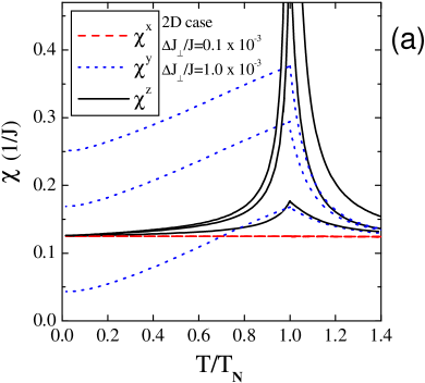
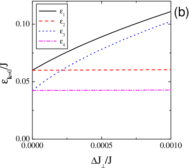
Figure 7: (Colour online) (a) All three components of the susceptibility within the RPA analytical scheme for different values of the interplanar anisotropy $\Delta J_{\perp}$: 2D result – upper curve, $\Delta J_{\perp}/J=0.1\times 10^{-3}$ – middle curve, and $\Delta J_{\perp}/J=1.0\times 10^{-3}$ – top curve; and the (b) $T=0$ energy gaps vs. the interplanar anisotropy $\Delta J_{\perp}$, for $d/J=0.058$, $\Delta\Gamma/J=0.42\times 10^{-3}$.

We also find that gap $\varepsilon_{1}$ is always greater than $\varepsilon_{2}$, and $\varepsilon_{3}$ is always greater than $\varepsilon_{4}$, when $\Delta J_{\perp}=J_{\perp}-J^{\prime}_{\perp}>0$ (indeed, that is the only case considered in this paper - see the discussion of figure 1 in section 2). As was mentioned above, the two modes $\varepsilon_{1}$, $\varepsilon_{2}$ describe the in-plane modes of the spectrum, while the modes $\varepsilon_{3}$, $\varepsilon_{4}$ describe the out-of-plane spin-wave excitations. Therefore, we find that the observed ratio between the $x$ and $y$ components $\chi^{x}<\chi^{y}$ (in the $T=0$ limit) [1], in any of the MFA, LSW theory, or the RPA, takes place only if the spin-wave gaps have the following hierarchy:

$$\varepsilon_{1}>\varepsilon_{2}>\varepsilon_{3}>\varepsilon_{4},$$ (1ca)

i.e. the in-plane modes ($\varepsilon_{1,2}$) are greater than the out-of-plane ones ($\varepsilon_{3,4}$).

The described situation is presented in figure 7 – they show the susceptibility for the different values of the interplanar parameter $\Delta J_{\perp}$. The upper curve was obtained for the pure 2D case and corresponds to the situation with the observed order of the susceptibility components $\chi^{x}<\chi^{y}$ and the following ordering of the gaps $\varepsilon_{1}=\varepsilon_{2}>\varepsilon_{3}=\varepsilon_{4}$. By increasing the magnitude of the interplanar parameter $\Delta J_{\perp}$ two modes $\varepsilon_{1}$ and $\varepsilon_{3}$ increase and the hierarchy of the gaps (1ca) remains unchanged (figure 7b). As we can see from the middle curve in figure 7a, the ratio $\chi^{y}/\chi^{x}$ decreases as the ratio between the gaps $\varepsilon_{2}/\varepsilon_{3}$ decreases. The magnitude of the out-of-plane mode $\varepsilon_{3}$ becomes equal to the in-plane one $\varepsilon_{2}$ when $\Delta J_{\perp}/J\approx\frac{1}{2}\big{(}\frac{1}{4}(d/J)^{2}-\Delta\Gamma/J\big{)}\approx 2.1\times 10^{-4}$, where the ratio $\chi^{y}/\chi^{x}$ goes to unity. A further increasing of $\Delta J_{\perp}$ changes the ratio between the modes $\varepsilon_{2}/\varepsilon_{3}$, and according to equation (1bx) changes the order of the susceptibility components $x,z$ and $y$ at zero temperature (see the lowest curve in figure 7a and the corresponding value of the gaps at $\Delta J_{\perp}=0.001$ in figure 7b).

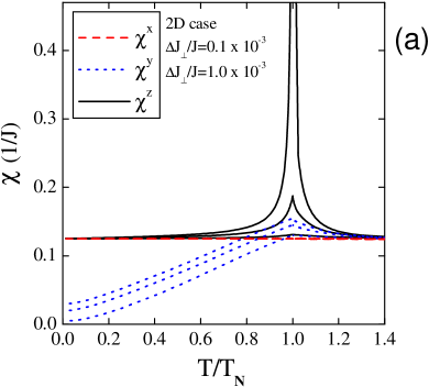
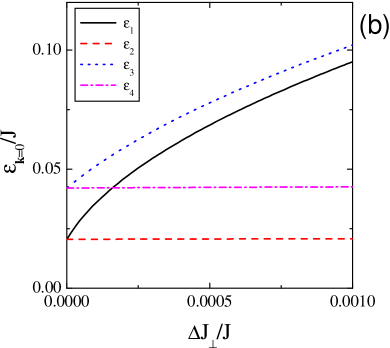
Figure 8: (Colour online) (a) All three components of the susceptibility within the RPA analytical scheme for different values of the interplanar anisotropy $\Delta J_{\perp}$: 2D result – upper curve, $\Delta J_{\perp}/J=0.1\times 10^{-3}$ –middle curve, and $\Delta J_{\perp}/J=1.0\times 10^{-3}$ – top curve; and the (b) $T=0$ energy gaps vs. the interplanar anisotropy $\Delta J_{\perp}$, for $d/J=0.02$, $\Delta\Gamma/J=0.42\times 10^{-3}$.

For completeness, in figure 8 we present the susceptibility and behaviour of the gaps vs. $\Delta J_{\perp}$ for smaller magnitudes of the in-plane anisotropy. We find that the interplanar coupling introduced into the problem leads to a suppression of the 2D quantum fluctuations caused by intraplanar anisotropies. For the large magnitude of $\Delta J_{\perp}=10^{-3}$, i.e. $\Delta J_{\perp}\sim 2\Delta\Gamma\ll d$, the net interplanar coupling $\Delta J_{\perp}$ dominates over the DM and XY-like pseudo-dipolar anisotropies (see the lower curve in figure 8a).

Finally, we conclude the presentation of these numerical results by returning to a discussion of the correlation between the magnitude of the zone-centre spin-wave gaps and the behaviour of the components $\chi^{x,z}$, $\chi^{y}$. One can see that only when $\varepsilon_{3}$ is greater than $\varepsilon_{2}$ at zero interplanar coupling $\Delta J_{\perp}=0$ does the $y$ component of the susceptibility at $T=0$ become less than components $\chi^{x,z}$, since the ratio between gaps remains unchanged for any values of $\Delta J_{\perp}$ (see equation (1bz)).

4 Approximate simple tetragonal model

For the model parameters of interest our initial Hamiltonian (1) can be approximated by a simple tetragonal model Hamiltonian which includes the intraplanar isotropic Heisenberg interaction $J$, the anisotropic DM term ${\bf D}$ that alternates in sign from bond to bond, the XY-like pseudo-dipolar anisotropy $\Delta\Gamma$, and an effective interplanar interaction $J^{eff}_{\perp}$. This effective model is defined by

$$H = \sum_{\langle i,j\rangle}[J{\bf S}_{i}\cdot{\bf S}_{j}-\Delta\Gamma S^{z}_{i}S^{z}_{j}+{\bf D}_{ij}\cdot({\bf S}_{i}\times{\bf S}_{j})]+\sum_{\langle k,k^{\prime}\rangle}J^{eff}_{\perp}{\bf S}_{k}\cdot{\bf S}_{k^{\prime}}~{}~{}.$$ (1cb)

The single-plane effective Hamiltonian was proposed by Peters et al. [16] long ago, and its reliability was demonstrated in our previous work [3]. Here the interplanar coupling $J^{eff}_{\perp}$ is added phenomenologically for a simple tetragonal lattice (see figure 9), $i$ and $j$ are nearest-neighbour sites in the same CuO plane (indexes $i_{1},j_{1}$ and $i_{2},j_{2}$ in figure 9) and $k$, $k^{\prime}$ are nearest-neighbour sites in adjacent planes (indexes $i_{1},i_{2}$ and $j_{1},j_{2}$ in figure 9). Since the interplanar coordination number for interplanar interaction within a simple tetragonal model is half that of the corresponding one for the coupling $\Delta J_{\perp}$, we can approximate $J^{eff}_{\perp}=2\Delta J_{\perp}$.

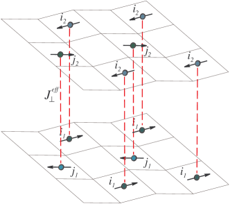
Figure 9: (Colour online) Magnetic structure of the simple tetragonal lattice described by the effective model Hamiltonian of equation (1cb). Use of this Hamiltonian for this lattice accurately approximates the magnetic response of the La₂CuO₄ crystal in the LTO phase.

We performed the calculations of the order parameter, spin-wave excitations and susceptibility within the RPA scheme for the effective simple tetragonal model of equation (1cb), and found that the transition temperature, spectrum, and behaviour of the order parameter and susceptibility almost identical to that on the initial model of equation (1). In figure 10 we show representative data for the susceptibility obtained for the initial body-centred orthorhombic model as well as for the effective simple tetragonal one with $J^{eff}_{\perp}=2\Delta J_{\perp}$ – clearly, the agreement between the predictions for these two models is excellent, so when studying the magnetic properties of the model (1) on 3D body-centred orthorhombic lattice one can utilize the effective Hamiltonian of the simple tetragonal lattice. Consequently, the magnetism of the La₂CuO₄ system in the LTO phase can be modelled by the Hamiltonian of equation (1cb).

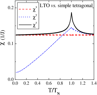
Figure 10: (Colour online) The susceptibility, in units of $1/J$, as a function of $T/T_{N}$. We present both results from the RPA calculation on the initial model Hamiltonian of equation (1) with $\Delta J_{\perp}/J=0.1\times 10^{-3}$ and the simple tetragonal model with the Hamiltonian of equation (1cb) with $J^{eff}_{\perp}/J=0.2\times 10^{-3}$ (for $d/J=0.02$ and $\Delta\Gamma/J=0.42\times 10^{-3}$). The curves from these two models essentially coincide, and no differences can seen on this scale.

5 Conclusions and Discussion

In this paper we presented a theoretical investigation of the body-centred orthorhombic lattice Heisenberg antiferromagnet with in-plane symmetric and anti-symmetric anisotropies, and a weak anisotropic AFM interlayer coupling. Our study was focused on the role of the different interactions in explaining the magnetic properties of a La₂CuO₄ crystal in the low-temperature orthorhombic (LTO) phase. Due to the transition into the orthorhombic phase, the AFM interplanar coupling between nearest-neighbour spins in the adjacent CuO₂ planes exhibits a small anisotropy. We have found that such a small anisotropy plays an important role in magnetic properties of the system. In figures 7a, 8a one sees a significant change in the behaviour of magnetic susceptibility as a function of temperature by varying the magnitude of the net interplanar coupling $\Delta J_{\perp}$. We also obtained that the (larger) individual superexchange interaction between any two nearest-neighbour spins in the adjacent planes does not affect the physics of the model (figure 3).

Our results have shown that in the case of an isotropic interplanar coupling, 2D quantum fluctuations dominate over the effects of the 3D interaction, and the transition to the long-range magnetically ordered state, as well as the behaviour of the susceptibility, order parameter and magnon excitation spectrum, are not influenced by the interplanar exchange coupling (however, for a 3D model the $z$ component of the susceptibility will not diverge, as it does in a 2D model). Thus, in the case of the body-centred lattice model of equation (1) with an isotropic interplanar coupling ($J^{\prime}_{\perp}=J_{\perp}$) one can analyze the system using a 2D square lattice model with intraplanar anisotropies only.

We have also obtained that the initial model Hamiltonian (1) can be effectively replaced by a simpler one with fewer model parameters, namely by the AFM Heisenberg Hamiltonian with DM interaction, XY-like pseudo-dipolar anisotropy, and an effective interplanar interaction $J^{eff}_{\perp}$ (added phenomenologically for a simple tetragonal lattice). Here $J^{eff}_{\perp}/2\sim 10^{-4}$ describes the small anisotropy of the AFM interplanar coupling in the initial system.

We emphasize an important conclusion that can be drawn from our results. We have found that in-plane anisotropy introduced into the problem by symmetric XY-like pseudo-dipolar and antisymmetric DM interactions largely determines the behaviour of the magnetic susceptibility, transition temperature into the long-range order state, and the spin-wave gaps in the case of a 3D model (within the wide range of model parameters of interest). Further, even when one studies a 3D model, the effect of quantum fluctuations is very strong in all temperature regions below the transition temperature, and cannot be ignored. Similar to the results of our previous paper [3], we have also obtained the large short-range correlations in the broad temperature region above the Néel temperature.

Now we comment on the comparison of our results to the experimentally observed anisotropies of the susceptibility [1] and spin-wave gaps [15] that motivated our work. We can state that all anisotropic interactions involved in the model, i.e. DM, XY-like pseudo-dipolar, and interplanar ones, are responsible for the unusual anisotropy in the magnetic susceptibility, and the appearance of gaps in spin-wave excitation spectrum. More concretely, by comparing to a purely 2D model, the inclusion of interplanar anisotropy leads to the splitting of either of the in- and out-of plane zone-centre spin-wave modes. While the neutron-scattering experiments find only two gaps, one in-plane mode $\varepsilon_{i}\approx 2.3$ meV and one out-of plane mode $\varepsilon_{o}\approx 5$ meV, we can infer the following possible situation that is predicted from our results: the in-plane mode $\varepsilon_{1}$ (which is always larger than $\varepsilon_{2}$) has a gap with a magnitude of about 10 meV. Indeed, such an in-plane gap can be seen from the result for the spin-wave spectra in the neutron-scattering experiments [15]; other observed gaps corresponds to the out-of plane mode $\varepsilon_{3}\approx 5$ meV and in-plane mode $\varepsilon_{2}\approx 2.3$ meV. The magnitude of the gap of the remaining out-of plane mode, $\varepsilon_{4}$, is relatively small and apparently has not be seen by experiment. Therefore the following hierarchy $\varepsilon_{1}>\varepsilon_{3}>\varepsilon_{2}>\varepsilon_{4}$ agrees with the experiment. In this paper we established the correlation between the ratio of the in and out-of-plane gaps of the excitation spectrum and the behaviour of $\chi^{x,z}$ and $\chi^{y}$ components of susceptibility in the zero temperature limit. However, the proposed hierarchy of the spin-wave gaps takes place only if the ratio between the $x$ and $y$ components is opposite to that observed in experiment ($\chi^{x}<\chi^{y}$). This necessarily leads to the question, would other interactions, e.g. ring exchange and/or the interaction between the next nearest neighbour sites [6], lead to an accurate explanation of the susceptibility data within the RPA scheme?

In order to answer this question we have performed calculation for the square lattice AFM Heisenberg model with the DM and XY-like pseudo-dipolar anisotropies by additionally taking into account the ring exchange and the interactions between the next nearest neighbour sites (for the energy scales of these additional interactions see reference [6]). Our results of the RPA calculations have established that ring exchange together with the second and third nearest neighbour in-plane exchanges do not change the results presented in our earlier paper [3] regarding the correlation between the ratio of the in and out-of-plane spin-wave modes gaps and the behaviour of the $\chi^{x}$ and $\chi^{y}$ components of susceptibility in the zero-$T$ limit, viz. $\varepsilon_{o}^{2}/\varepsilon_{i}^{2}\approx\chi^{x}/\chi^{y}$. So, physics beyond what has been presented in our previous and this manuscript is important, but that does not imply that a more complicated Hamiltonian with more interactions is necessarily required.

A potential resolution of this dilemma can be found in studies based on the quantum non-linear sigma model [14]. However, within a theory that accounts for short-wavelength behaviour we will show in a future publication how the “next” approximation beyond that used in our previous [3] and present papers fits the experimental data. This allows for the important next problem of the coupling of the anisotropic AFM state to either localized or mobile holes to be examined.

Appendix A Characteristic representation

The transformation between the initial representation and the characteristic representation (CR) in which the quantization axis $\sigma^{z}$ is in the direction of the classical moment (see figure 1) reads

$$\left(\begin{array}[]{c}\sigma_{i_{1}}^{x}\\ \sigma_{i_{1}}^{y}\\ \sigma_{i_{1}}^{z}\\ \end{array}\right) = \frac{1}{\sqrt{2}}\left(\begin{array}[]{ccc}1&\sin\theta&-\cos\theta\\ -1&\sin\theta&-\cos\theta\\ 0&\sqrt{2}\cos\theta&\sqrt{2}\sin\theta\\ \end{array}\right)\left(\begin{array}[]{c}S_{i_{1}}^{x}\\ S_{i_{1}}^{y}\\ S_{i_{1}}^{z}\\ \end{array}\right),$$ (1cl)

$$\left(\begin{array}[]{c}\sigma_{j_{1}}^{x}\\ \sigma_{j_{1}}^{y}\\ \sigma_{j_{1}}^{z}\\ \end{array}\right) = \frac{1}{\sqrt{2}}\left(\begin{array}[]{ccc}1&\sin\theta&\cos\theta\\ -1&\sin\theta&\cos\theta\\ 0&-\sqrt{2}\cos\theta&\sqrt{2}\sin\theta\\ \end{array}\right)\left(\begin{array}[]{c}S_{j_{1}}^{x}\\ S_{j_{1}}^{y}\\ S_{j_{1}}^{z}\\ \end{array}\right),$$ (1cv)

$$\left(\begin{array}[]{c}\sigma_{i_{2}}^{x}\\ \sigma_{i_{2}}^{y}\\ \sigma_{i_{2}}^{z}\\ \end{array}\right) = \frac{1}{\sqrt{2}}\left(\begin{array}[]{ccc}1&-\sin\theta&\cos\theta\\ -1&-\sin\theta&\cos\theta\\ 0&-\sqrt{2}\cos\theta&-\sqrt{2}\sin\theta\\ \end{array}\right)\left(\begin{array}[]{c}S_{i_{2}}^{x}\\ S_{i_{2}}^{y}\\ S_{i_{2}}^{z}\\ \end{array}\right),$$ (1df)

$$\left(\begin{array}[]{c}\sigma_{j_{2}}^{x}\\ \sigma_{j_{2}}^{y}\\ \sigma_{j_{2}}^{z}\\ \end{array}\right) = \frac{1}{\sqrt{2}}\left(\begin{array}[]{ccc}1&-\sin\theta&-\cos\theta\\ -1&-\sin\theta&-\cos\theta\\ 0&\sqrt{2}\cos\theta&-\sqrt{2}\sin\theta\\ \end{array}\right)\left(\begin{array}[]{c}S_{j_{2}}^{x}\\ S_{j_{2}}^{y}\\ S_{j_{2}}^{z}\\ \end{array}\right).$$ (1dp)

In our calculations we formally divided the body-centred lattice into the four sublattices which differ in orientation of their spins within the ground state. As was explained in section 2, we follow the notation where $i_{1}$-sites belong to sublattice 1, $j_{1}$-sites to sublattice 2, $i_{2}$-sites to sublattice 3, and $j_{2}$-sites to sublattice 4, respectively.

By using the CR as the basic representation we obtain the components of susceptibility that determine the response of the expectation value of the spins in one sublattice with respect to the external magnetic field applied to another one. For instance, the component

$$\chi^{\sigma^{x}\sigma^{y}}_{13}\equiv\frac{4}{N}\frac{\partial}{\partial h_{3}^{y}}\sum^{N/4}_{i_{1}=1}\langle\sigma_{i_{1}}^{x}\rangle=\frac{4}{N}\sum^{N/4}_{i_{1}=1}\sum^{N/4}_{i_{2}=1}\int^{\beta}_{0}\!\!\langle T_{\tau}\sigma_{i_{1}}^{x}(\tau)\sigma_{i_{2}}^{y}(0)\rangle{\rm d}\tau~{}~{},$$ (1dq)

determines the response of the expectation value of the spin $\sigma^{x}$, $4/N\sum^{N/4}_{i_{1}}\langle\sigma_{i_{1}}^{x}\rangle$, in sublattice ’1’ to the field applied to sublattice ’3’ in the $\sigma^{y}$-direction of the corresponding coordinate system within the CR [3].

The transformation between the susceptibility components in the initial and CR coordinates reads

$$\chi^{x} = \frac{1}{2}\{\chi^{\sigma^{x}\sigma^{x}}_{11}+\chi^{\sigma^{x}\sigma^{x}}_{12}+\chi^{\sigma^{x}\sigma^{x}}_{13}+\chi^{\sigma^{x}\sigma^{x}}_{14}-\chi^{\sigma^{x}\sigma^{y}}_{11}-\chi^{\sigma^{x}\sigma^{y}}_{12}-\chi^{\sigma^{x}\sigma^{y}}_{13}-\chi^{\sigma^{x}\sigma^{y}}_{14}$$ (1dr)

$$+\chi^{\sigma^{y}\sigma^{y}}_{11}+\chi^{\sigma^{y}\sigma^{y}}_{12}+\chi^{\sigma^{y}\sigma^{y}}_{13}+\chi^{\sigma^{y}\sigma^{y}}_{14}-\chi^{\sigma^{y}\sigma^{x}}_{11}-\chi^{\sigma^{y}\sigma^{x}}_{12}-\chi^{\sigma^{y}\sigma^{x}}_{13}-\chi^{\sigma^{y}\sigma^{x}}_{14}\},$$

$$\chi^{y} = \frac{\sin^{2}(\theta)}{2}\{\chi^{\sigma^{x}\sigma^{x}}_{11}+\chi^{\sigma^{x}\sigma^{x}}_{12}-\chi^{\sigma^{x}\sigma^{x}}_{13}-\chi^{\sigma^{x}\sigma^{x}}_{14}+\chi^{\sigma^{x}\sigma^{y}}_{11}+\chi^{\sigma^{x}\sigma^{y}}_{12}-\chi^{\sigma^{x}\sigma^{y}}_{13}-\chi^{\sigma^{x}\sigma^{y}}_{14}$$ (1ds)

$$\qquad+\chi^{\sigma^{y}\sigma^{y}}_{11}+\chi^{\sigma^{y}\sigma^{y}}_{12}-\chi^{\sigma^{y}\sigma^{y}}_{13}-\chi^{\sigma^{y}\sigma^{y}}_{14}+\chi^{\sigma^{y}\sigma^{x}}_{11}+\chi^{\sigma^{y}\sigma^{x}}_{12}-\chi^{\sigma^{y}\sigma^{x}}_{13}-\chi^{\sigma^{y}\sigma^{x}}_{14}\}$$

$$+ \cos^{2}(\theta)\{\chi^{\sigma^{z}\sigma^{z}}_{11}-\chi^{\sigma^{z}\sigma^{z}}_{12}-\chi^{\sigma^{z}\sigma^{z}}_{13}+\chi^{\sigma^{z}\sigma^{z}}_{14}\},$$

$$\chi^{z} = \frac{\cos^{2}(\theta)}{2}\{\chi^{\sigma^{x}\sigma^{x}}_{11}-\chi^{\sigma^{x}\sigma^{x}}_{12}-\chi^{\sigma^{x}\sigma^{x}}_{13}+\chi^{\sigma^{x}\sigma^{x}}_{14}+\chi^{\sigma^{x}\sigma^{y}}_{11}-\chi^{\sigma^{x}\sigma^{y}}_{12}-\chi^{\sigma^{x}\sigma^{y}}_{13}+\chi^{\sigma^{x}\sigma^{y}}_{14}$$ (1dt)

$$\qquad+\chi^{\sigma^{y}\sigma^{y}}_{11}-\chi^{\sigma^{y}\sigma^{y}}_{12}-\chi^{\sigma^{y}\sigma^{y}}_{13}+\chi^{\sigma^{y}\sigma^{y}}_{14}+\chi^{\sigma^{y}\sigma^{x}}_{11}-\chi^{\sigma^{y}\sigma^{x}}_{12}-\chi^{\sigma^{y}\sigma^{x}}_{13}+\chi^{\sigma^{y}\sigma^{x}}_{14}\}$$

$$+ \sin^{2}(\theta)\{\chi^{\sigma^{z}\sigma^{z}}_{11}+\chi^{\sigma^{z}\sigma^{z}}_{12}-\chi^{\sigma^{z}\sigma^{z}}_{13}-\chi^{\sigma^{z}\sigma^{z}}_{14}\}.$$

Appendix B System of equations for the Green’s functions in the momentum-frequency representation

Let us present the most general form of the system of equations for the Green’s function’s in equation (1ae). We introduce notation $g$ for the zero-order $g_{ln}=G_{ln}(\boldsymbol{k},\omega_{m})$ and/or first-order $g_{ln}=G^{(1)}_{ln}(\boldsymbol{k},\omega_{m})$ Green’s functions depending on the coefficients in the equations (see below). Then, the system reads

$$\frac{{\rm{i}}\omega_{m}}{2{\cal Z}\eta}g_{12} = \hphantom{-}U_{12}+\frac{J_{mfa}}{2}g_{12}+A_{\boldsymbol{k}}g_{22}-B_{\boldsymbol{k}}g^{-}_{22}+a_{\boldsymbol{k}}g_{42}-{\rm{i}}b_{\boldsymbol{k}}g^{-}_{42}-{\rm{i}}d_{\boldsymbol{k}}g^{-}_{32}~{}~{},$$

$$\frac{{\rm{i}}\omega_{m}}{2{\cal Z}\eta}g_{22} = \hphantom{-}U_{22}+\frac{J_{mfa}}{2}g_{22}+A_{\boldsymbol{k}}g_{12}-B_{\boldsymbol{k}}g^{-}_{12}+a_{\boldsymbol{k}}g_{32}-{\rm{i}}b_{\boldsymbol{k}}g^{-}_{32}-{\rm{i}}d_{\boldsymbol{k}}g^{-}_{42}~{}~{},$$

$$\frac{{\rm{i}}\omega_{m}}{2{\cal Z}\eta}g^{-}_{12} = -U^{-}_{12}-\frac{J_{mfa}}{2}g^{-}_{12}-A_{\boldsymbol{k}}g^{-}_{22}+B^{*}_{\boldsymbol{k}}g_{22}-a_{\boldsymbol{k}}g^{-}_{42}-{\rm{i}}b_{\boldsymbol{k}}g_{42}-{\rm{i}}d_{\boldsymbol{k}}g_{32}~{}~{},$$

$$\frac{{\rm{i}}\omega_{m}}{2{\cal Z}\eta}g^{-}_{22} = -U^{-}_{22}-\frac{J_{mfa}}{2}g^{-}_{22}-A_{\boldsymbol{k}}g^{-}_{12}+B^{*}_{\boldsymbol{k}}g_{12}-a_{\boldsymbol{k}}g^{-}_{32}-{\rm{i}}b_{\boldsymbol{k}}g_{32}-{\rm{i}}d_{\boldsymbol{k}}g_{42}~{}~{},$$ (1du)

$$\frac{{\rm{i}}\omega_{m}}{2{\cal Z}\eta}g_{32} = \hphantom{-}U_{32}+\frac{J_{mfa}}{2}g_{32}+A_{\boldsymbol{k}}g_{42}+B^{*}_{\boldsymbol{k}}g^{-}_{42}+a_{\boldsymbol{k}}g_{22}-{\rm{i}}b_{\boldsymbol{k}}g^{-}_{22}-{\rm{i}}d_{\boldsymbol{k}}g^{-}_{12}~{}~{},$$

$$\frac{{\rm{i}}\omega_{m}}{2{\cal Z}\eta}g_{42} = \hphantom{-}U_{42}+\frac{J_{mfa}}{2}g_{42}+A_{\boldsymbol{k}}g_{32}+B^{*}_{\boldsymbol{k}}g^{-}_{32}+a_{\boldsymbol{k}}g_{12}-{\rm{i}}b_{\boldsymbol{k}}g^{-}_{12}-{\rm{i}}d_{\boldsymbol{k}}g^{-}_{22}~{}~{},$$

$$\frac{{\rm{i}}\omega_{m}}{2{\cal Z}\eta}g^{-}_{32} = -U^{-}_{32}-\frac{J_{mfa}}{2}g^{-}_{32}-A_{\boldsymbol{k}}g^{-}_{42}-B_{\boldsymbol{k}}g_{42}-a_{\boldsymbol{k}}g^{-}_{22}-{\rm{i}}b_{\boldsymbol{k}}g_{22}-{\rm{i}}d_{\boldsymbol{k}}g_{12}~{}~{},$$

$$\frac{{\rm{i}}\omega_{m}}{2{\cal Z}\eta}g^{-}_{42} = -U^{-}_{42}-\frac{J_{mfa}}{2}g^{-}_{42}-A_{\boldsymbol{k}}g^{-}_{32}-B_{\boldsymbol{k}}g_{32}-a_{\boldsymbol{k}}g^{-}_{12}-{\rm{i}}b_{\boldsymbol{k}}g_{12}-{\rm{i}}d_{\boldsymbol{k}}g_{22}~{}~{}.$$

In the case of the zero-order system, $g_{ln}=G_{ln}(\boldsymbol{k},\omega_{m})$, we have

$$U_{22}=-\frac{1}{\cal Z},\quad U_{12}=U^{-}_{12}=U^{-}_{22}=U_{32}=U_{42}=U^{-}_{32}=U^{-}_{42}=0.$$ (1dv)

In case of the first-order system $g_{ln}=G^{(1)}_{ln}(\boldsymbol{k},\omega_{m})$ we have

$$U_{12}=V_{12}G_{12}=\bigg{\{}\frac{1}{2{\cal Z}\eta}{+}\frac{J_{2}}{2}\frac{\rm{v}_{2}}{\eta}+\frac{J_{\perp}}{2}\frac{\rm{v}_{3}}{\eta}-\frac{J_{p}}{2}\frac{\rm{v}_{4}}{\eta}+\bigg{(}\frac{{\rm{i}}\omega}{2{\cal Z}\eta}{-}\frac{J_{mfa}}{2}\bigg{)}\frac{\rm{v}_{1}}{\eta}\bigg{\}}G_{12},$$

$$U_{22}=V_{22}G_{22}=\bigg{\{}\hphantom{\frac{1}{2{\cal Z}\eta}+}\frac{J_{2}}{2}\frac{\rm{v}_{1}}{\eta}+\frac{J_{\perp}}{2}\frac{\rm{v}_{4}}{\eta}-\frac{J_{p}}{2}\frac{\rm{v}_{3}}{\eta}+\bigg{(}\frac{{\rm{i}}\omega}{2{\cal Z}\eta}{-}\frac{J_{mfa}}{2}\bigg{)}\frac{\rm{v}_{2}}{\eta}\bigg{\}}G_{22},$$

$$U^{-}_{12}=V^{-}_{12}G^{-}_{12}=\bigg{\{}\frac{1}{2{\cal Z}\eta}{+}\frac{J_{2}}{2}\frac{\rm{v}_{2}}{\eta}+\frac{J_{\perp}}{2}\frac{\rm{v}_{3}}{\eta}-\frac{J_{p}}{2}\frac{\rm{v}_{4}}{\eta}-\bigg{(}\frac{{\rm{i}}\omega}{2{\cal Z}\eta}{+}\frac{J_{mfa}}{2}\bigg{)}\frac{\rm{v}_{1}}{\eta}\bigg{\}}G^{-}_{12},$$

$$U^{-}_{22}=V^{-}_{22}G^{-}_{22}=\bigg{\{}\hphantom{\frac{1}{2{\cal Z}\eta}+}\frac{J_{2}}{2}\frac{\rm{v}_{1}}{\eta}+\frac{J_{\perp}}{2}\frac{\rm{v}_{4}}{\eta}-\frac{J_{p}}{2}\frac{\rm{v}_{3}}{\eta}-\bigg{(}\frac{{\rm{i}}\omega}{2{\cal Z}\eta}{+}\frac{J_{mfa}}{2}\bigg{)}\frac{\rm{v}_{2}}{\eta}\bigg{\}}G^{-}_{22},$$ (1dw)

$$U_{32}=V_{32}G_{32}=\bigg{\{}\hphantom{\frac{1}{2{\cal Z}\eta}+}\frac{J_{2}}{2}\frac{\rm{v}_{4}}{\eta}+\frac{J_{\perp}}{2}\frac{\rm{v}_{1}}{\eta}-\frac{J_{p}}{2}\frac{\rm{v}_{2}}{\eta}+\bigg{(}\frac{{\rm{i}}\omega}{2{\cal Z}\eta}{-}\frac{J_{mfa}}{2}\bigg{)}\frac{\rm{v}_{3}}{\eta}\bigg{\}}G_{32},$$

$$U_{42}=V_{42}G_{42}=\bigg{\{}\hphantom{\frac{1}{2{\cal Z}\eta}+}\frac{J_{2}}{2}\frac{\rm{v}_{3}}{\eta}+\frac{J_{\perp}}{2}\frac{\rm{v}_{2}}{\eta}-\frac{J_{p}}{2}\frac{\rm{v}_{1}}{\eta}+\bigg{(}\frac{{\rm{i}}\omega}{2{\cal Z}\eta}{-}\frac{J_{mfa}}{2}\bigg{)}\frac{\rm{v}_{4}}{\eta}\bigg{\}}G_{42},$$

$$U^{-}_{32}=V^{-}_{32}G^{-}_{32}=\bigg{\{}\hphantom{\frac{1}{2{\cal Z}\eta}+}\frac{J_{2}}{2}\frac{\rm{v}_{4}}{\eta}+\frac{J_{\perp}}{2}\frac{\rm{v}_{1}}{\eta}-\frac{J_{p}}{2}\frac{\rm{v}_{2}}{\eta}-\bigg{(}\frac{{\rm{i}}\omega}{2{\cal Z}\eta}{+}\frac{J_{mfa}}{2}\bigg{)}\frac{\rm{v}_{3}}{\eta}\bigg{\}}G^{-}_{32},$$

$$U^{-}_{42}=V^{-}_{42}G^{-}_{42}=\bigg{\{}\hphantom{\frac{1}{2{\cal Z}\eta}+}\frac{J_{2}}{2}\frac{\rm{v}_{3}}{\eta}+\frac{J_{\perp}}{2}\frac{\rm{v}_{2}}{\eta}-\frac{J_{p}}{2}\frac{\rm{v}_{1}}{\eta}-\bigg{(}\frac{{\rm{i}}\omega}{2{\cal Z}\eta}{+}\frac{J_{mfa}}{2}\bigg{)}\frac{\rm{v}_{4}}{\eta}\bigg{\}}G^{-}_{42};$$

where the new quantities $V_{ln}$ and $V^{-}_{ln}$ were introduced.

Appendix C Zero-order Green’s functions

For ease of presentation, we define some new quantities:

$$x_{1,\boldsymbol{k}}=-2a_{\boldsymbol{k}}[a_{\boldsymbol{k}}(A_{\boldsymbol{k}}{-}J_{mfa}/2)-(b_{\boldsymbol{k}}{-}d_{\boldsymbol{k}})\Im B_{\boldsymbol{k}}],\qquad y_{1,\boldsymbol{k}}=-(A_{\boldsymbol{k}}{-}J_{mfa}/2),$$

$$x_{2,\boldsymbol{k}}=\hphantom{-}2a_{\boldsymbol{k}}[a_{\boldsymbol{k}}(A_{\boldsymbol{k}}{+}J_{mfa}/2)-(b_{\boldsymbol{k}}{+}d_{\boldsymbol{k}})\Im B_{\boldsymbol{k}}],\qquad y_{2,\boldsymbol{k}}=\hphantom{-}(A_{\boldsymbol{k}}{+}J_{mfa}/2),$$

$$x_{3,\boldsymbol{k}}=2\Re B_{\boldsymbol{k}}[-a^{2}_{\boldsymbol{k}}+(b_{\boldsymbol{k}}{-}d_{\boldsymbol{k}})^{2}]+2{\rm{i}}(b_{\boldsymbol{k}}{-}d_{\boldsymbol{k}})[\hphantom{-}a_{\boldsymbol{k}}(A_{\boldsymbol{k}}{-}J_{mfa}/2)-\Im B_{\boldsymbol{k}}(b_{\boldsymbol{k}}{-}d_{\boldsymbol{k}})],$$

$$x_{4,\boldsymbol{k}}=2\Re B_{\boldsymbol{k}}[\hphantom{-}a^{2}_{\boldsymbol{k}}-(b_{\boldsymbol{k}}{+}d_{\boldsymbol{k}})^{2}]+2{\rm{i}}(b_{\boldsymbol{k}}{+}d_{\boldsymbol{k}})[-a_{\boldsymbol{k}}(A_{\boldsymbol{k}}{+}J_{mfa}/2)+\Im B_{\boldsymbol{k}}(b_{\boldsymbol{k}}{+}d_{\boldsymbol{k}})],$$

$$y_{3,\boldsymbol{k}}=-B^{*}_{\boldsymbol{k}},$$

$$y_{4,\boldsymbol{k}}=\hphantom{-}B^{*}_{\boldsymbol{k}},$$

$$x_{5,\boldsymbol{k}}=-2(A_{\boldsymbol{k}}{-}J_{mfa}/2)[a_{\boldsymbol{k}}(A_{\boldsymbol{k}}{-}J_{mfa}/2)-(b_{\boldsymbol{k}}{-}d_{\boldsymbol{k}})\Im B_{\boldsymbol{k}}]+2a_{\boldsymbol{k}}\Re^{2}B_{\boldsymbol{k}},$$

$$\hskip 28.45274pt+2{\rm{i}}\Re B_{\boldsymbol{k}}[(A_{\boldsymbol{k}}{-}J_{mfa}/2)(b_{\boldsymbol{k}}{-}d_{\boldsymbol{k}})-a_{\boldsymbol{k}}\Im B_{\boldsymbol{k}}],$$

$$x_{6,\boldsymbol{k}}=\hphantom{-}2(A_{\boldsymbol{k}}{+}J_{mfa}/2)[a_{\boldsymbol{k}}(A_{\boldsymbol{k}}{+}J_{mfa}/2)-(b_{\boldsymbol{k}}{+}d_{\boldsymbol{k}})\Im B_{\boldsymbol{k}}]-2a_{\boldsymbol{k}}\Re^{2}B_{\boldsymbol{k}},$$

$$\hskip 28.45274pt-2{\rm{i}}\Re B_{\boldsymbol{k}}[(A_{\boldsymbol{k}}{+}J_{mfa}/2)(b_{\boldsymbol{k}}{+}d_{\boldsymbol{k}})-a_{\boldsymbol{k}}\Im B_{\boldsymbol{k}}],$$

$$y_{5,\boldsymbol{k}}=-a_{\boldsymbol{k}},\qquad z_{5,\boldsymbol{k}}=-2\Im B_{\boldsymbol{k}}(b_{\boldsymbol{k}}{-}d_{\boldsymbol{k}})+2a_{\boldsymbol{k}}(A_{\boldsymbol{k}}{-}J_{mfa}/2)-2{\rm{i}}\Re B_{\boldsymbol{k}}(b_{\boldsymbol{k}}{-}d_{\boldsymbol{k}}),$$

$$y_{6,\boldsymbol{k}}=\hphantom{-}a_{\boldsymbol{k}},\qquad z_{6,\boldsymbol{k}}=-2\Im B_{\boldsymbol{k}}(b_{\boldsymbol{k}}{+}d_{\boldsymbol{k}})+2a_{\boldsymbol{k}}(A_{\boldsymbol{k}}{+}J_{mfa}/2)-2{\rm{i}}\Re B_{\boldsymbol{k}}(b_{\boldsymbol{k}}{+}d_{\boldsymbol{k}}),$$

$$x_{7,\boldsymbol{k}}=\hphantom{-}2{\rm{i}}[a_{\boldsymbol{k}}(A_{\boldsymbol{k}}{-}J_{mfa}/2)\Im B_{\boldsymbol{k}}-(b_{\boldsymbol{k}}{-}d_{\boldsymbol{k}})|B_{\boldsymbol{k}}|^{2}],$$

$$x_{8,\boldsymbol{k}}=-2{\rm{i}}[a_{\boldsymbol{k}}(A_{\boldsymbol{k}}{+}J_{mfa}/2)\Im B_{\boldsymbol{k}}-(b_{\boldsymbol{k}}{+}d_{\boldsymbol{k}})|B_{\boldsymbol{k}}|^{2}],$$

$$y_{7,\boldsymbol{k}}=\hphantom{-}{\rm{i}}(b_{\boldsymbol{k}}{-}d_{\boldsymbol{k}}),\qquad z_{7,\boldsymbol{k}}=-2a_{\boldsymbol{k}}\Re B_{\boldsymbol{k}},$$

$$y_{8,\boldsymbol{k}}=-{\rm{i}}(b_{\boldsymbol{k}}{+}d_{\boldsymbol{k}}),\qquad z_{8,\boldsymbol{k}}=-2a_{\boldsymbol{k}}\Re B_{\boldsymbol{k}}.$$

Then, the solution of the system of equations for the zero-order Green’s functions can be written as

$$G_{12}(\boldsymbol{k},\omega_{m})=\frac{\eta}{4}\bigg{\{}\!\! \frac{1}{\omega_{1,\boldsymbol{k}}}\bigg{(}\frac{\omega_{1,\boldsymbol{k}}{+}y_{1,\boldsymbol{k}}{+}x_{1,\boldsymbol{k}}/\sqrt{\beta_{1,\boldsymbol{k}}}}{{\rm{i}}\omega_{m}-\varepsilon_{1,\boldsymbol{k}}}+\frac{\omega_{1,\boldsymbol{k}}{-}y_{1,\boldsymbol{k}}{-}x_{1,\boldsymbol{k}}/\sqrt{\beta_{1,\boldsymbol{k}}}}{{\rm{i}}\omega_{m}+\varepsilon_{1,\boldsymbol{k}}}\bigg{)}$$

$$+ \frac{1}{\omega_{2,\boldsymbol{k}}}\bigg{(}\frac{\omega_{2,\boldsymbol{k}}{+}y_{1,\boldsymbol{k}}{-}x_{1,\boldsymbol{k}}/\sqrt{\beta_{1,\boldsymbol{k}}}}{{\rm{i}}\omega_{m}-\varepsilon_{2,\boldsymbol{k}}}+\frac{\omega_{2,\boldsymbol{k}}{-}y_{1,\boldsymbol{k}}{+}x_{1,\boldsymbol{k}}/\sqrt{\beta_{1,\boldsymbol{k}}}}{{\rm{i}}\omega_{m}+\varepsilon_{2,\boldsymbol{k}}}\bigg{)}$$

$$- \frac{1}{\omega_{3,\boldsymbol{k}}}\bigg{(}\frac{\omega_{3,\boldsymbol{k}}{+}y_{2,\boldsymbol{k}}{+}x_{2,\boldsymbol{k}}/\sqrt{\beta_{2,\boldsymbol{k}}}}{{\rm{i}}\omega_{m}-\varepsilon_{3,\boldsymbol{k}}}+\frac{\omega_{3,\boldsymbol{k}}{-}y_{2,\boldsymbol{k}}{-}x_{2,\boldsymbol{k}}/\sqrt{\beta_{2,\boldsymbol{k}}}}{{\rm{i}}\omega_{m}+\varepsilon_{3,\boldsymbol{k}}}\bigg{)}$$

$$- \frac{1}{\omega_{4,\boldsymbol{k}}}\bigg{(}\frac{\omega_{4,\boldsymbol{k}}{+}y_{2,\boldsymbol{k}}{-}x_{2,\boldsymbol{k}}/\sqrt{\beta_{2,\boldsymbol{k}}}}{{\rm{i}}\omega_{m}-\varepsilon_{4,\boldsymbol{k}}}+\frac{\omega_{4,\boldsymbol{k}}{-}y_{2,\boldsymbol{k}}{+}x_{2,\boldsymbol{k}}/\sqrt{\beta_{2,\boldsymbol{k}}}}{{\rm{i}}\omega_{m}+\varepsilon_{4,\boldsymbol{k}}}\bigg{)}\bigg{\}}~{}~{},$$

$$G_{22}(\boldsymbol{k},\omega_{m})=\frac{\eta}{4}\bigg{\{}\!\! - \frac{1}{\omega_{1,\boldsymbol{k}}}\bigg{(}\frac{\omega_{1,\boldsymbol{k}}{+}y_{1,\boldsymbol{k}}{+}x_{1,\boldsymbol{k}}/\sqrt{\beta_{1,\boldsymbol{k}}}}{{\rm{i}}\omega_{m}-\varepsilon_{1,\boldsymbol{k}}}+\frac{\omega_{1,\boldsymbol{k}}{-}y_{1,\boldsymbol{k}}{-}x_{1,\boldsymbol{k}}/\sqrt{\beta_{1,\boldsymbol{k}}}}{{\rm{i}}\omega_{m}+\varepsilon_{1,\boldsymbol{k}}}\bigg{)}$$

$$- \frac{1}{\omega_{2,\boldsymbol{k}}}\bigg{(}\frac{\omega_{2,\boldsymbol{k}}{+}y_{1,\boldsymbol{k}}{-}x_{1,\boldsymbol{k}}/\sqrt{\beta_{1,\boldsymbol{k}}}}{{\rm{i}}\omega_{m}-\varepsilon_{2,\boldsymbol{k}}}+\frac{\omega_{2,\boldsymbol{k}}{-}y_{1,\boldsymbol{k}}{+}x_{1,\boldsymbol{k}}/\sqrt{\beta_{1,\boldsymbol{k}}}}{{\rm{i}}\omega_{m}+\varepsilon_{2,\boldsymbol{k}}}\bigg{)}$$

$$- \frac{1}{\omega_{3,\boldsymbol{k}}}\bigg{(}\frac{\omega_{3,\boldsymbol{k}}{+}y_{2,\boldsymbol{k}}{+}x_{2,\boldsymbol{k}}/\sqrt{\beta_{2,\boldsymbol{k}}}}{{\rm{i}}\omega_{m}-\varepsilon_{3,\boldsymbol{k}}}+\frac{\omega_{3,\boldsymbol{k}}{-}y_{2,\boldsymbol{k}}{-}x_{2,\boldsymbol{k}}/\sqrt{\beta_{2,\boldsymbol{k}}}}{{\rm{i}}\omega_{m}+\varepsilon_{3,\boldsymbol{k}}}\bigg{)}$$

$$- \frac{1}{\omega_{4,\boldsymbol{k}}}\bigg{(}\frac{\omega_{4,\boldsymbol{k}}{+}y_{2,\boldsymbol{k}}{-}x_{2,\boldsymbol{k}}/\sqrt{\beta_{2,\boldsymbol{k}}}}{{\rm{i}}\omega_{m}-\varepsilon_{4,\boldsymbol{k}}}+\frac{\omega_{4,\boldsymbol{k}}{-}y_{2,\boldsymbol{k}}{+}x_{2,\boldsymbol{k}}/\sqrt{\beta_{2,\boldsymbol{k}}}}{{\rm{i}}\omega_{m}+\varepsilon_{4,\boldsymbol{k}}}\bigg{)}\bigg{\}}$$

$$G^{-}_{12}(\boldsymbol{k},\omega_{m})=\frac{\eta}{4}\bigg{\{}\!\! \frac{1}{\omega_{1,\boldsymbol{k}}}\bigg{(}\frac{y_{3,\boldsymbol{k}}{+}x_{3,\boldsymbol{k}}/\sqrt{\beta_{1,\boldsymbol{k}}}}{{\rm{i}}\omega_{m}-\varepsilon_{1,\boldsymbol{k}}}+\frac{-y_{3,\boldsymbol{k}}{-}x_{3,\boldsymbol{k}}/\sqrt{\beta_{1,\boldsymbol{k}}}}{{\rm{i}}\omega_{m}+\varepsilon_{1,\boldsymbol{k}}}\bigg{)}$$

$$+ \frac{1}{\omega_{2,\boldsymbol{k}}}\bigg{(}\frac{y_{3,\boldsymbol{k}}{-}x_{3,\boldsymbol{k}}/\sqrt{\beta_{1,\boldsymbol{k}}}}{{\rm{i}}\omega_{m}-\varepsilon_{2,\boldsymbol{k}}}+\frac{-y_{3,\boldsymbol{k}}{+}x_{3,\boldsymbol{k}}/\sqrt{\beta_{1,\boldsymbol{k}}}}{{\rm{i}}\omega_{m}+\varepsilon_{2,\boldsymbol{k}}}\bigg{)}$$

$$- \frac{1}{\omega_{3,\boldsymbol{k}}}\bigg{(}\frac{y_{4,\boldsymbol{k}}{+}x_{4,\boldsymbol{k}}/\sqrt{\beta_{2,\boldsymbol{k}}}}{{\rm{i}}\omega_{m}-\varepsilon_{3,\boldsymbol{k}}}+\frac{-y_{4,\boldsymbol{k}}{-}x_{4,\boldsymbol{k}}/\sqrt{\beta_{2,\boldsymbol{k}}}}{{\rm{i}}\omega_{m}+\varepsilon_{3,\boldsymbol{k}}}\bigg{)}$$

$$- \frac{1}{\omega_{4,\boldsymbol{k}}}\bigg{(}\frac{y_{4,\boldsymbol{k}}{-}x_{4,\boldsymbol{k}}/\sqrt{\beta_{2,\boldsymbol{k}}}}{{\rm{i}}\omega_{m}-\varepsilon_{4,\boldsymbol{k}}}+\frac{-y_{4,\boldsymbol{k}}{+}x_{4,\boldsymbol{k}}/\sqrt{\beta_{2,\boldsymbol{k}}}}{{\rm{i}}\omega_{m}+\varepsilon_{4,\boldsymbol{k}}}\bigg{)}\bigg{\}}$$

$$G^{-}_{22}(\boldsymbol{k},\omega_{m})=\frac{\eta}{4}\bigg{\{}\!\! - \frac{1}{\omega_{1,\boldsymbol{k}}}\bigg{(}\frac{y_{3,\boldsymbol{k}}{+}x_{3,\boldsymbol{k}}/\sqrt{\beta_{1,\boldsymbol{k}}}}{{\rm{i}}\omega_{m}-\varepsilon_{1,\boldsymbol{k}}}+\frac{-y_{3,\boldsymbol{k}}{-}x_{3,\boldsymbol{k}}/\sqrt{\beta_{1,\boldsymbol{k}}}}{{\rm{i}}\omega_{m}+\varepsilon_{1,\boldsymbol{k}}}\bigg{)}$$

$$- \frac{1}{\omega_{2,\boldsymbol{k}}}\bigg{(}\frac{y_{3,\boldsymbol{k}}{-}x_{3,\boldsymbol{k}}/\sqrt{\beta_{1,\boldsymbol{k}}}}{{\rm{i}}\omega_{m}-\varepsilon_{2,\boldsymbol{k}}}+\frac{-y_{3,\boldsymbol{k}}{+}x_{3,\boldsymbol{k}}/\sqrt{\beta_{1,\boldsymbol{k}}}}{{\rm{i}}\omega_{m}+\varepsilon_{2,\boldsymbol{k}}}\bigg{)}$$

$$- \frac{1}{\omega_{3,\boldsymbol{k}}}\bigg{(}\frac{y_{4,\boldsymbol{k}}{+}x_{4,\boldsymbol{k}}/\sqrt{\beta_{2,\boldsymbol{k}}}}{{\rm{i}}\omega_{m}-\varepsilon_{3,\boldsymbol{k}}}+\frac{-y_{4,\boldsymbol{k}}{-}x_{4,\boldsymbol{k}}/\sqrt{\beta_{2,\boldsymbol{k}}}}{{\rm{i}}\omega_{m}+\varepsilon_{3,\boldsymbol{k}}}\bigg{)}$$

$$- \frac{1}{\omega_{4,\boldsymbol{k}}}\bigg{(}\frac{y_{4,\boldsymbol{k}}{-}x_{4,\boldsymbol{k}}/\sqrt{\beta_{2,\boldsymbol{k}}}}{{\rm{i}}\omega_{m}-\varepsilon_{4,\boldsymbol{k}}}+\frac{-y_{4,\boldsymbol{k}}{+}x_{4,\boldsymbol{k}}/\sqrt{\beta_{2,\boldsymbol{k}}}}{{\rm{i}}\omega_{m}+\varepsilon_{4,\boldsymbol{k}}}\bigg{)}\bigg{\}}$$

$$G_{32}(\boldsymbol{k},\omega_{m})=\frac{\eta}{4}\bigg{\{}\!\! \frac{1}{\omega_{1,\boldsymbol{k}}}\bigg{(}\frac{y_{5,\boldsymbol{k}}{+}(x_{5,\boldsymbol{k}}{+}z_{5,\boldsymbol{k}}\omega_{1,\boldsymbol{k}})/\sqrt{\beta_{1,\boldsymbol{k}}}}{{\rm{i}}\omega_{m}-\varepsilon_{1,\boldsymbol{k}}}+\frac{{-}y_{5,\boldsymbol{k}}{-}(x_{5,\boldsymbol{k}}{-}z_{5,\boldsymbol{k}}\omega_{1,\boldsymbol{k}})/\sqrt{\beta_{1,\boldsymbol{k}}}}{{\rm{i}}\omega_{m}+\varepsilon_{1,\boldsymbol{k}}}\bigg{)}$$

$$+ \frac{1}{\omega_{2,\boldsymbol{k}}}\bigg{(}\frac{y_{5,\boldsymbol{k}}{-}(x_{5,\boldsymbol{k}}{+}z_{5,\boldsymbol{k}}\omega_{2,\boldsymbol{k}})/\sqrt{\beta_{1,\boldsymbol{k}}}}{{\rm{i}}\omega_{m}-\varepsilon_{2,\boldsymbol{k}}}+\frac{{-}y_{5,\boldsymbol{k}}{+}(x_{5,\boldsymbol{k}}{-}z_{5,\boldsymbol{k}}\omega_{2,\boldsymbol{k}})/\sqrt{\beta_{1,\boldsymbol{k}}}}{{\rm{i}}\omega_{m}+\varepsilon_{2,\boldsymbol{k}}}\bigg{)}$$

$$- \frac{1}{\omega_{3,\boldsymbol{k}}}\bigg{(}\frac{y_{6,\boldsymbol{k}}{+}(x_{6,\boldsymbol{k}}{+}z_{6,\boldsymbol{k}}\omega_{3,\boldsymbol{k}})/\sqrt{\beta_{2,\boldsymbol{k}}}}{{\rm{i}}\omega_{m}-\varepsilon_{3,\boldsymbol{k}}}+\frac{{-}y_{6,\boldsymbol{k}}{-}(x_{6,\boldsymbol{k}}{-}z_{6,\boldsymbol{k}}\omega_{3,\boldsymbol{k}})/\sqrt{\beta_{2,\boldsymbol{k}}}}{{\rm{i}}\omega_{m}+\varepsilon_{3,\boldsymbol{k}}}\bigg{)}$$

$$- \frac{1}{\omega_{4,\boldsymbol{k}}}\bigg{(}\frac{y_{6,\boldsymbol{k}}{-}(x_{6,\boldsymbol{k}}{+}z_{6,\boldsymbol{k}}\omega_{4,\boldsymbol{k}})/\sqrt{\beta_{2,\boldsymbol{k}}}}{{\rm{i}}\omega_{m}-\varepsilon_{4,\boldsymbol{k}}}+\frac{{-}y_{6,\boldsymbol{k}}{+}(x_{6,\boldsymbol{k}}{-}z_{6,\boldsymbol{k}}\omega_{4,\boldsymbol{k}})/\sqrt{\beta_{2,\boldsymbol{k}}}}{{\rm{i}}\omega_{m}+\varepsilon_{4,\boldsymbol{k}}}\bigg{)}\bigg{\}}$$

$$G_{42}(\boldsymbol{k},\omega_{m})=\frac{\eta}{4}\bigg{\{}\!\! - \frac{1}{\omega_{1,\boldsymbol{k}}}\bigg{(}\frac{y_{5,\boldsymbol{k}}{+}(x_{5,\boldsymbol{k}}{+}z_{5,\boldsymbol{k}}\omega_{1,\boldsymbol{k}})/\sqrt{\beta_{1,\boldsymbol{k}}}}{{\rm{i}}\omega_{m}-\varepsilon_{1,\boldsymbol{k}}}+\frac{{-}y_{5,\boldsymbol{k}}{-}(x_{5,\boldsymbol{k}}{-}z_{5,\boldsymbol{k}}\omega_{1,\boldsymbol{k}})/\sqrt{\beta_{1,\boldsymbol{k}}}}{{\rm{i}}\omega_{m}+\varepsilon_{1,\boldsymbol{k}}}\bigg{)}$$

$$- \frac{1}{\omega_{2,\boldsymbol{k}}}\bigg{(}\frac{y_{5,\boldsymbol{k}}{-}(x_{5,\boldsymbol{k}}{+}z_{5,\boldsymbol{k}}\omega_{2,\boldsymbol{k}})/\sqrt{\beta_{1,\boldsymbol{k}}}}{{\rm{i}}\omega_{m}-\varepsilon_{2,\boldsymbol{k}}}+\frac{{-}y_{5,\boldsymbol{k}}{+}(x_{5,\boldsymbol{k}}{-}z_{5,\boldsymbol{k}}\omega_{2,\boldsymbol{k}})/\sqrt{\beta_{1,\boldsymbol{k}}}}{{\rm{i}}\omega_{m}+\varepsilon_{2,\boldsymbol{k}}}\bigg{)}$$

$$- \frac{1}{\omega_{3,\boldsymbol{k}}}\bigg{(}\frac{y_{6,\boldsymbol{k}}{+}(x_{6,\boldsymbol{k}}{+}z_{6,\boldsymbol{k}}\omega_{3,\boldsymbol{k}})/\sqrt{\beta_{2,\boldsymbol{k}}}}{{\rm{i}}\omega_{m}-\varepsilon_{3,\boldsymbol{k}}}+\frac{{-}y_{6,\boldsymbol{k}}{-}(x_{6,\boldsymbol{k}}{-}z_{6,\boldsymbol{k}}\omega_{3,\boldsymbol{k}})/\sqrt{\beta_{2,\boldsymbol{k}}}}{{\rm{i}}\omega_{m}+\varepsilon_{3,\boldsymbol{k}}}\bigg{)}$$

$$- \frac{1}{\omega_{4,\boldsymbol{k}}}\bigg{(}\frac{y_{6,\boldsymbol{k}}{-}(x_{6,\boldsymbol{k}}{+}z_{6,\boldsymbol{k}}\omega_{4,\boldsymbol{k}})/\sqrt{\beta_{2,\boldsymbol{k}}}}{{\rm{i}}\omega_{m}-\varepsilon_{4,\boldsymbol{k}}}+\frac{{-}y_{6,\boldsymbol{k}}{+}(x_{6,\boldsymbol{k}}{-}z_{6,\boldsymbol{k}}\omega_{4,\boldsymbol{k}})/\sqrt{\beta_{2,\boldsymbol{k}}}}{{\rm{i}}\omega_{m}+\varepsilon_{4,\boldsymbol{k}}}\bigg{)}\bigg{\}}$$

$$G^{-}_{32}(\boldsymbol{k},\omega_{m})=\frac{\eta}{4}\bigg{\{}\!\! \frac{1}{\omega_{1,\boldsymbol{k}}}\bigg{(}\frac{y_{7,\boldsymbol{k}}{+}(x_{7,\boldsymbol{k}}{+}z_{7,\boldsymbol{k}}\omega_{1,\boldsymbol{k}})/\sqrt{\beta_{1,\boldsymbol{k}}}}{{\rm{i}}\omega_{m}-\varepsilon_{1,\boldsymbol{k}}}+\frac{{-}y_{7,\boldsymbol{k}}{-}(x_{7,\boldsymbol{k}}{-}z_{7,\boldsymbol{k}}\omega_{1,\boldsymbol{k}})/\sqrt{\beta_{1,\boldsymbol{k}}}}{{\rm{i}}\omega_{m}+\varepsilon_{1,\boldsymbol{k}}}\bigg{)}$$

$$+ \frac{1}{\omega_{2,\boldsymbol{k}}}\bigg{(}\frac{y_{7,\boldsymbol{k}}{-}(x_{7,\boldsymbol{k}}{+}z_{7,\boldsymbol{k}}\omega_{2,\boldsymbol{k}})/\sqrt{\beta_{1,\boldsymbol{k}}}}{{\rm{i}}\omega_{m}-\varepsilon_{2,\boldsymbol{k}}}+\frac{{-}y_{7,\boldsymbol{k}}{+}(x_{7,\boldsymbol{k}}{-}z_{7,\boldsymbol{k}}\omega_{2,\boldsymbol{k}})/\sqrt{\beta_{1,\boldsymbol{k}}}}{{\rm{i}}\omega_{m}+\varepsilon_{2,\boldsymbol{k}}}\bigg{)}$$

$$- \frac{1}{\omega_{3,\boldsymbol{k}}}\bigg{(}\frac{y_{8,\boldsymbol{k}}{+}(x_{8,\boldsymbol{k}}{+}z_{8,\boldsymbol{k}}\omega_{3,\boldsymbol{k}})/\sqrt{\beta_{2,\boldsymbol{k}}}}{{\rm{i}}\omega_{m}-\varepsilon_{3,\boldsymbol{k}}}+\frac{{-}y_{8,\boldsymbol{k}}{-}(x_{8,\boldsymbol{k}}{-}z_{8,\boldsymbol{k}}\omega_{3,\boldsymbol{k}})/\sqrt{\beta_{2,\boldsymbol{k}}}}{{\rm{i}}\omega_{m}+\varepsilon_{3,\boldsymbol{k}}}\bigg{)}$$

$$- \frac{1}{\omega_{4,\boldsymbol{k}}}\bigg{(}\frac{y_{8,\boldsymbol{k}}{-}(x_{8,\boldsymbol{k}}{+}z_{8,\boldsymbol{k}}\omega_{4,\boldsymbol{k}})/\sqrt{\beta_{2,\boldsymbol{k}}}}{{\rm{i}}\omega_{m}-\varepsilon_{4,\boldsymbol{k}}}+\frac{{-}y_{8,\boldsymbol{k}}{+}(x_{8,\boldsymbol{k}}{-}z_{8,\boldsymbol{k}}\omega_{4,\boldsymbol{k}})/\sqrt{\beta_{2,\boldsymbol{k}}}}{{\rm{i}}\omega_{m}+\varepsilon_{4,\boldsymbol{k}}}\bigg{)}\bigg{\}}$$

$$G^{-}_{42}(\boldsymbol{k},\omega_{m})=\frac{\eta}{4}\bigg{\{}\!\! -\frac{1}{\omega_{1,\boldsymbol{k}}}\bigg{(}\frac{y_{7,\boldsymbol{k}}{+}(x_{7,\boldsymbol{k}}{+}z_{7,\boldsymbol{k}}\omega_{1,\boldsymbol{k}})/\sqrt{\beta_{1,\boldsymbol{k}}}}{{\rm{i}}\omega_{m}-\varepsilon_{1,\boldsymbol{k}}}+\frac{{-}y_{7,\boldsymbol{k}}{-}(x_{7,\boldsymbol{k}}{-}z_{7,\boldsymbol{k}}\omega_{1,\boldsymbol{k}})/\sqrt{\beta_{1,\boldsymbol{k}}}}{{\rm{i}}\omega_{m}+\varepsilon_{1,\boldsymbol{k}}}\bigg{)}$$

$$- \frac{1}{\omega_{2,\boldsymbol{k}}}\bigg{(}\frac{y_{7,\boldsymbol{k}}{-}(x_{7,\boldsymbol{k}}{+}z_{7,\boldsymbol{k}}\omega_{2,\boldsymbol{k}})/\sqrt{\beta_{1,\boldsymbol{k}}}}{{\rm{i}}\omega_{m}-\varepsilon_{2,\boldsymbol{k}}}+\frac{{-}y_{7,\boldsymbol{k}}{+}(x_{7,\boldsymbol{k}}{-}z_{7,\boldsymbol{k}}\omega_{2,\boldsymbol{k}})/\sqrt{\beta_{1,\boldsymbol{k}}}}{{\rm{i}}\omega_{m}+\varepsilon_{2,\boldsymbol{k}}}\bigg{)}$$

$$- \frac{1}{\omega_{3,\boldsymbol{k}}}\bigg{(}\frac{y_{8,\boldsymbol{k}}{+}(x_{8,\boldsymbol{k}}{+}z_{8,\boldsymbol{k}}\omega_{3,\boldsymbol{k}})/\sqrt{\beta_{2,\boldsymbol{k}}}}{{\rm{i}}\omega_{m}-\varepsilon_{3,\boldsymbol{k}}}+\frac{{-}y_{8,\boldsymbol{k}}{-}(x_{8,\boldsymbol{k}}{-}z_{8,\boldsymbol{k}}\omega_{3,\boldsymbol{k}})/\sqrt{\beta_{2,\boldsymbol{k}}}}{{\rm{i}}\omega_{m}+\varepsilon_{3,\boldsymbol{k}}}\bigg{)}$$

$$- \frac{1}{\omega_{4,\boldsymbol{k}}}\bigg{(}\frac{y_{8,\boldsymbol{k}}{-}(x_{8,\boldsymbol{k}}{+}z_{8,\boldsymbol{k}}\omega_{4,\boldsymbol{k}})/\sqrt{\beta_{2,\boldsymbol{k}}}}{{\rm{i}}\omega_{m}-\varepsilon_{4,\boldsymbol{k}}}+\frac{{-}y_{8,\boldsymbol{k}}{+}(x_{8,\boldsymbol{k}}{-}z_{8,\boldsymbol{k}}\omega_{4,\boldsymbol{k}})/\sqrt{\beta_{2,\boldsymbol{k}}}}{{\rm{i}}\omega_{m}+\varepsilon_{4,\boldsymbol{k}}}\bigg{)}\bigg{\}}$$

Appendix D First-order Green’s functions

From the whole set of the first-order Green’s functions we need only the diagonal $G^{(1)}_{ll}$ ones. The solution for such Green’s functions can be presented via the coefficients $V_{ln}$ (defined in equation (1dw)) and zero-order Green’s functions in the following form:

$$G^{(1)}_{11}=-{\cal Z}\left\{\>|G_{12}|^{2}V_{22}+|G_{22}|^{2}V_{12}+|G^{-}_{12}|^{2}V^{-}_{22}+|G^{-}_{22}|^{2}V^{-}_{12}\right.$$ (1ef)

$$\hskip 45.52458pt\left.\>+|G_{32}|^{2}V_{42}+|G_{42}|^{2}V_{32}+|G^{-}_{32}|^{2}V^{-}_{42}+|G^{-}_{42}|^{2}V^{-}_{32}\>\right\}$$

$$G^{(1)}_{22}=-{\cal Z}\left\{\>|G_{12}|^{2}V_{12}+|G_{22}|^{2}V_{22}+|G^{-}_{12}|^{2}V^{-}_{12}+|G^{-}_{22}|^{2}V^{-}_{22}\right.$$ (1eg)

$$\hskip 45.52458pt\left.\>+|G_{32}|^{2}V_{32}+|G_{42}|^{2}V_{42}+|G^{-}_{32}|^{2}V^{-}_{32}+|G^{-}_{42}|^{2}V^{-}_{42}\>\right\}$$

$$G^{(1)}_{33}=-{\cal Z}\left\{\>|G_{12}|^{2}V_{42}+|G_{22}|^{2}V_{32}+|G^{-}_{12}|^{2}V^{-}_{42}+|G^{-}_{22}|^{2}V^{-}_{32}\right.$$ (1eh)

$$\hskip 45.52458pt\left.\>+|G_{32}|^{2}V_{22}+|G_{42}|^{2}V_{12}+|G^{-}_{32}|^{2}V^{-}_{22}+|G^{-}_{42}|^{2}V^{-}_{12}\>\right\}$$

$$G^{(1)}_{44}=-{\cal Z}\left\{\>|G_{12}|^{2}V_{32}+|G_{22}|^{2}V_{42}+|G^{-}_{12}|^{2}V^{-}_{32}+|G^{-}_{22}|^{2}V^{-}_{42}\right.$$ (1ei)

$$\hskip 45.52458pt\left.\>+|G_{32}|^{2}V_{12}+|G_{42}|^{2}V_{22}+|G^{-}_{32}|^{2}V^{-}_{12}+|G^{-}_{42}|^{2}V^{-}_{22}\>\right\}$$

Appendix E Transverse components of the susceptibility in the characteristic representation

We can find the transverse components of susceptibility from the following relations

$$\chi^{\sigma^{x}\sigma^{x}}_{ln} = \frac{1}{2}\{\hphantom{-}\Re\chi^{\sigma^{+}\sigma^{-}}_{ln}+\Re\chi^{\sigma^{-}\sigma^{-}}_{ln}\},\quad\chi^{\sigma^{y}\sigma^{y}}_{ln}=\frac{1}{2}\{\Re\chi^{\sigma^{+}\sigma^{-}}_{ln}-\Re\chi^{\sigma^{-}\sigma^{-}}_{ln}\},$$ (1ej)

$$\chi^{\sigma^{x}\sigma^{y}}_{ln} = \frac{1}{2}\{-\Im\chi^{\sigma^{+}\sigma^{-}}_{ln}-\Im\chi^{\sigma^{-}\sigma^{-}}_{ln}\},\quad\chi^{\sigma^{y}\sigma^{x}}_{ln}=\frac{1}{2}\{\Im\chi^{\sigma^{+}\sigma^{-}}_{ln}-\Im\chi^{\sigma^{-}\sigma^{-}}_{ln}\}~{}~{},$$ (1ek)

for any sublattice $l,n=1,2,3,4$. The components $\chi^{\sigma^{+}\sigma^{-}}\!,$ $\chi^{\sigma^{-}\sigma^{-}}$ can be found immediately from the solution of the zero-order Green’s functions in C and the definition in equation (1bd) with $\alpha=+,-$:

$$\chi^{\sigma^{+}\sigma^{-}}_{11}=\frac{1}{4{\cal Z}}\bigg{\{}\!\! \frac{y_{1}{+}x_{1}/\sqrt{\beta_{1}}}{\omega^{2}_{1}}+\frac{y_{1}{-}x_{1}/\sqrt{\beta_{1}}}{\omega^{2}_{2}}+\frac{y_{2}{+}x_{2}/\sqrt{\beta_{2}}}{\omega^{2}_{3}}+\frac{y_{2}{-}x_{2}/\sqrt{\beta_{2}}}{\omega^{2}_{4}}\bigg{\}},$$ (1el)

$$\chi^{\sigma^{+}\sigma^{-}}_{12}=\frac{1}{4{\cal Z}}\bigg{\{}\!\! - \frac{y_{1}{+}x_{1}/\sqrt{\beta_{1}}}{\omega^{2}_{1}}-\frac{y_{1}{-}x_{1}/\sqrt{\beta_{1}}}{\omega^{2}_{2}}+\frac{y_{2}{+}x_{2}/\sqrt{\beta_{2}}}{\omega^{2}_{3}}+\frac{y_{2}{-}x_{2}/\sqrt{\beta_{2}}}{\omega^{2}_{4}}\bigg{\}},$$ (1em)

$$\chi^{\sigma^{+}\sigma^{-}}_{13}=\frac{1}{4{\cal Z}}\bigg{\{}\!\! \frac{y_{5}{+}x_{5}/\sqrt{\beta_{1}}}{\omega^{2}_{1}}+\frac{y_{5}{-}x_{5}/\sqrt{\beta_{1}}}{\omega^{2}_{2}}+\frac{y_{6}{+}x_{6}/\sqrt{\beta_{2}}}{\omega^{2}_{3}}+\frac{y_{6}{-}x_{6}/\sqrt{\beta_{2}}}{\omega^{2}_{4}}\bigg{\}},$$ (1en)

$$\chi^{\sigma^{+}\sigma^{-}}_{14}=\frac{1}{4{\cal Z}}\bigg{\{}\!\! - \frac{y_{5}{+}x_{5}/\sqrt{\beta_{1}}}{\omega^{2}_{1}}-\frac{y_{5}{-}x_{5}/\sqrt{\beta_{1}}}{\omega^{2}_{2}}+\frac{y_{6}{+}x_{6}/\sqrt{\beta_{2}}}{\omega^{2}_{3}}+\frac{y_{6}{-}x_{6}/\sqrt{\beta_{2}}}{\omega^{2}_{4}}\bigg{\}},$$ (1eo)

$$\chi^{\sigma^{-}\sigma^{-}}_{11}=\frac{1}{4{\cal Z}}\bigg{\{}\!\! \frac{y_{3}{+}x_{3}/\sqrt{\beta_{1}}}{\omega^{2}_{1}}+\frac{y_{3}{-}x_{3}/\sqrt{\beta_{1}}}{\omega^{2}_{2}}+\frac{y_{4}{+}x_{4}/\sqrt{\beta_{2}}}{\omega^{2}_{3}}+\frac{y_{4}{-}x_{4}/\sqrt{\beta_{2}}}{\omega^{2}_{4}}\bigg{\}},$$ (1ep)

$$\chi^{\sigma^{-}\sigma^{-}}_{12}=\frac{1}{4{\cal Z}}\bigg{\{}\!\! - \frac{y_{3}{+}x_{3}/\sqrt{\beta_{1}}}{\omega^{2}_{1}}-\frac{y_{3}{-}x_{3}/\sqrt{\beta_{1}}}{\omega^{2}_{2}}+\frac{y_{4}{+}x_{4}/\sqrt{\beta_{2}}}{\omega^{2}_{3}}+\frac{y_{4}{-}x_{4}/\sqrt{\beta_{2}}}{\omega^{2}_{4}}\bigg{\}},$$ (1eq)

$$\chi^{\sigma^{-}\sigma^{-}}_{13}=\frac{1}{4{\cal Z}}\bigg{\{}\!\! \frac{y_{7}{+}x_{7}/\sqrt{\beta_{1}}}{\omega^{2}_{1}}+\frac{y_{7}{-}x_{7}/\sqrt{\beta_{1}}}{\omega^{2}_{2}}+\frac{y_{8}{+}x_{8}/\sqrt{\beta_{2}}}{\omega^{2}_{3}}+\frac{y_{8}{-}x_{8}/\sqrt{\beta_{2}}}{\omega^{2}_{4}}\bigg{\}},$$ (1er)

$$\chi^{\sigma^{-}\sigma^{-}}_{14}=\frac{1}{4{\cal Z}}\bigg{\{}\!\! - \frac{y_{7}{+}x_{7}/\sqrt{\beta_{1}}}{\omega^{2}_{1}}-\frac{y_{7}{-}x_{7}/\sqrt{\beta_{1}}}{\omega^{2}_{2}}+\frac{y_{8}{+}x_{8}/\sqrt{\beta_{2}}}{\omega^{2}_{3}}+\frac{y_{8}{-}x_{8}/\sqrt{\beta_{2}}}{\omega^{2}_{4}}\bigg{\}},$$ (1es)

where all coefficients $x_{l}$, $y_{l}$ with $l=1,\dots 8$, which are taken from the C, and all frequencies $\omega$, and $\beta_{1,2}$ (see equations (1au,1aw)) are taken in the long wavelength limit $\boldsymbol{k}\rightarrow 0$. Note that in above formulae we have also used the following relations between the different components of the transverse components of susceptibility in the CR

$$\chi_{11}=\chi_{22}=\chi_{33}=\chi_{44},\qquad\chi_{12}=\chi_{21}=\chi_{34}=\chi_{43},$$ (1et)

$$\chi_{13}=\chi_{31}=\chi_{42}=\chi_{24},\qquad\chi_{14}=\chi_{41}=\chi_{32}=\chi_{23}.$$

References

References

- [1] Lavrov A N, Ando Y, Komiya S and Tsukada I 2001 Phys. Rev. Lett., 87 0170071
- [2] Tranquada J M 2005 cond-mat/0508272
- [3] Tabunshchyk K V and Gooding R J 2005 Phys. Rev. B, 71 214418
- [4] Dzialoshinski I 1958 J. Phys. Chem. Solids, 4 241
- [5] Moriya T 1960 Phys. Rev., 120 91
- [6] Katanin A A and Kampf A P 2002 Phys. Rev. B 66, 100403(R)
- [7] Johnston David C 1997 Handbook of Magnetic Materials 10 (Elsevier, New York, 1997)
- [8] Coffey D, Rice T M and Zhang F C 1991 Phys. Rev. B, 44 10112
- [9] Shekhtman L, Ebtin-Wohlman O and Aharony A 1993 Phys. Rev. Lett., 71 468
- [10] Koshibae W, Ohta Y and Maekawa S 1994 Phys. Rev. B, 50 3767
- [11] Xue W, Grest G S, Cohen M H, Sinha S K and Soukoulis C 1988 Phys. Rev. B, 38 6868
- [12] Lee K H, Liu S H 1967 Phys. Rev., 159 390
- [13] Tyablikov S V 1959 Ukrain. Mat. Zh, 11 287
- [14] Silva Neto M B, Benfatto L, Juricic V and Morais Smith C 2005 cond-mat/0502588
- [15] Keimer B, Birgeneau R J, Cassanho A, Endoh Y, Greven M, Kastner M A and Shirane G 1993 Z. Phys. B, 91 373
- [16] Peters C J, Birgeneau R J, Kastner M A, Yoshizawa H, Endoh Y, Tranquada J, Shirane G, Hidaka Y, Oda M, Suzuki M and Murakami T 1988 Phys. Rev. B, 37 9761