Inhomogeneous sandpile model: Crossover from multifractal scaling to finite size scaling

Abstract

We study an inhomogeneous sandpile model in which two different toppling rules are defined. For any site only one rule is applied corresponding to either the Bak, Tang and Wiesenfeld model [P.Bak, C. Tang, and K. Wiesenfeld, Phys. Rev. Lett. 59, 381 (1987)] or the Manna two-state sandpile model [S. S. Manna, J. Phys. A 24, L363 (1991)]. A parameter $c$ is introduced which describes a density of sites which are randomly deployed and where the stochastic Manna rules are applied. The results show that the avalanche area exponent $\tau_{a}$, avalanche size exponent $\tau_{s}$, and capacity fractal dimension $D_{s}$ depend on the density $c$. A crossover from multifractal scaling of the Bak, Tang, and Wiesenfeld model ($c=0$) to finite size scaling was found. The critical density $c$ is found to be in the interval $0<c<0.01$. These results demonstrate that local dynamical rules are important and can change the global properties of the model.

I Introduction

Bak, Tang, and Wiesenfeld (BTW) BTW_1987 introduced a concept of self-organized criticality (SOC) as a common feature of different dynamical systems where the power-law temporal or spatial correlations are extended over several decades. Dynamical systems with many interacting degrees of freedom and with short range couplings naturally evolve into a critical state through a self-organized process. They proposed a simple cellular automaton with deterministic rules, which is known as a sandpile model, to demonstrate this new phenomenon. In this model the relaxation rules are conservative, no dissipation takes place during relaxation, and correspond to a nonlinear diffusion equation BTW_1987 . Generally, the sandpile model is represented by a $d$-dimensional hypercube of the finite linear size $L$. Its boundaries are open and allow an energy dissipation, which takes place only at the boundaries.

Manna proposed a two-state version of the sandpile model Manna_1991 where no more than one particle is allowed to be at a site in the stationary state. If one particle is added to a randomly chosen site, then relaxation starts depending on the occupancy of the site. If the site is empty, a particle is launched. In the case when the site is not empty, a hard core interaction throws the particles out from the site and the particles are redistributed in a random manner among its neighbours. All sites affected by this redistribution create an avalanche. An avalanche is stopped if any site reached the stationary state, i.e. no more than one particle occupies a site.

The first systematic study of scaling properties, universality and classification of deterministic sandpile models was carried out by Kadanoff et al. Kadanoff . Using numerical simulations and by varying the underlying microscopic rules which describe how an avalanche is generated they investigated whether different models have the same universal properties. Applying finite-size scaling (FSS) and multifractal scaling techniques they studied how a finite-size of the system affects scaling properties.

The real-space renormalization group calculations Pietronero suggested that deterministic BTW_1987 and stochastic Manna_1991 sandpile models belong to the same universality class. On the other hand, many numerical results Ben-Hur ; Biham ; Lubeck ; Menech ; Milsh show clearly two different universality classes. They do not confirm the hypothesis that small modifications in the dynamical rules of the models do not change the universality class, presented by Chessa at al. Chessa .

This study was motivated by the results published by Tebaldi et al. Tebaldi_1999 , and Stella and Menech Stella_2001 , where a multifractal scaling of an avalanche size distribution of the BTW model was demonstrated. They assume that a multifractal character for SOC models like the BTW model is a crucial step towards the solution of universality issues. By applying the moment analysis they found FSS for the two-state Manna model Stella_2001 . Based on these results they conclude that the 2D BTW model and the Manna model belong to qualitatively different universality classes. This assumption was confirmed recently Karma ; Karma_E , where a precise toppling balance has been investigated in more detail.

In this paper we report the results of disturbing the dynamics of the BTW model using stochastic Manna sites which are randomly deployed. They can introduce stochastic events during an avalanche propagation. Our model was derived from the inhomogeneous sandpile model Cer in witch two different deterministic toppling rules were defined. In the proposed model the first toppling rule corresponds to the BTW model BTW_1987 and the second rule is now stochastic and corresponds to the two-state Manna model Manna_1991 . The model is similar to that in Ref. Karma_E , however we applied the original toppling rules of the listed sandpile models.

The paper is organized as follows. The inhomogeneous sandpile model is introduced in Sec. II. The avalanche scaling exponents, capacity fractal dimensions and crossover from multifractal to FSS are investigated with numerical simulations and the results are presented in Sec. III. The Sec. IV is devoted to a discussion which is followed by conclusions in Sec. V.

II Mathematical model

We consider a $d$-dimensional hyper-cubic lattice of linear size $L$, and a notation presented by Ben-Hur et al. Ben-Hur is followed to define a sandpile model. Each site $\mathbf{\mathbf{i}}$ has assigned a dynamical variable $E(\mathbf{\mathbf{i}})$ that generally represents a physical quantity such as energy, grain density, stress, etc. A configuration $\{E(\mathbf{i})\}$ is classified as stable if for all sites $E(\mathbf{\mathbf{i}})<E_{c}$, where $E_{c}$ is a threshold value. We note that the two-state Manna model Manna_1991 has no threshold $E_{c}$. The Manna model has defined a hard core repulsion interaction among different particles at the same position. This hard core repulsion interaction can be described by a threshold where the threshold value $E_{c}=2$ is assigned to any site. In our inhomogeneous sandpile model, the threshold values $E_{c}$ depend on the site position $\mathbf{i}$, $E_{c}(\mathbf{i})$ Cer . The conditions for a stationary state, a stable configuration $\{E(\mathbf{i})\}$ (no avalanche), are now $E(\mathbf{i})<E_{c}(\mathbf{i})$, where the threshold $E_{c}(\mathbf{i})$ at the site $\mathbf{i}$ was randomly chosen from two allowed values

$$E_{c}(\mathbf{i})=\begin{cases}E_{c}^{I}\ =4\\ E_{c}^{II}=2.\end{cases}$$ (1)

For any site $\mathbf{i}$ the threshold $E_{c}(\mathbf{i})$ [Eq. (1)] is defined in such a manner that $n$ randomly chosen sites have the value $E_{c}^{II}$ and the remaining $L^{d}-n$ sites have the value $E_{c}^{I}$. The density of sites with the threshold value $E_{c}^{II}$ is denoted $c$, and $c=n/L^{d}$.

Let us assume that a stable configuration $\{E(\mathbf{j})\}$ is given, and then we select a site $\mathbf{i}$ at random and increase $E(\mathbf{i})$ by some amount $\delta E$. We now consider $\delta E=1$ for any site. When an unstable configuration is reached, $E(\mathbf{i})\geq E_{c}(\mathbf{i})$, a relaxation takes place. An unstable site $\mathbf{i}$ lowers its energy, that is distributed among the neighbor sites. The directions to the neighbor sites are defined by the vectors $\mathbf{e}_{1}=(0,1)$, $\mathbf{e}_{2}=(0,-1)$, $\mathbf{e}_{3}=(1,0)$, and $\mathbf{e}_{4}=(-1,0)$. The relaxation is defined by the following rules

$$E(\mathbf{i})\rightarrow E(\mathbf{i})-\sum_{e}\Delta E(\mathbf{i}),$$ (2)

$$E(\mathbf{i}+\mathbf{e})\rightarrow E(\mathbf{i}+\mathbf{e})+\Delta E(\mathbf{e}),$$ (3)

$$\sum_{e}\Delta E(\mathbf{e})=E_{c}(\mathbf{i}),$$ (4)

$$\mathbf{e}=\begin{cases}\{\mathbf{e}_{1},\ \mathbf{e}_{2},\ \mathbf{e}_{3},\ \mathbf{e}_{4}\}&if\ E_{c}(\mathbf{i})=E_{c}^{I}\\ \{\mathbf{e}_{\zeta},\ \mathbf{e}_{\eta}\}&if\ E_{c}(\mathbf{i})=E_{c}^{II}\end{cases}$$ (5)

where $\mathbf{e}$ is a set of vectors from the site $\mathbf{i}$ to its neighbors. The indexes $\zeta$ and $\eta$ are integers $1,2,3$, and $4$ randomly chosen at any relaxation. The neighbors that receive the energy can became unstable and topple, thus generating an avalanche. The distribution of energy is described by Eqs. (2) and (3), we added additional rules Eqs. (4) and (5) which specify the manner how the energy is distributed depending on the position $\mathbf{i}$, threshold $E_{c}(\mathbf{i})$ [Eq. (4)], and corresponding sandpile model [Eq. (5)]. The relaxation rules Eqs. (2)-(5) are applied until that moment when a new stable configuration is reached again, for all sites $E(\mathbf{i})<E_{c}(\mathbf{i})$. Obviously, during one avalanche an arbitrary unstable site $\mathbf{i}$ can transfer the energy $E_{c}(\mathbf{i})$ a few times to became stable, $E(\mathbf{i})<E_{c}(\mathbf{i})$. A $d$-dimensional lattice has open boundaries so added energy can flow outside the system, and an energy dissipation takes place only at the boundaries.

This model has been designed to enable a well defined change between two well known nondirected sandpile models: deterministic BTW_1987 and stochastic Manna_1991 (nondirected only on average) similarly as in Ref. Karma . The model belongs to the critical height models with conservative relaxation rules and with undirected energy transfer where the two thresholds are randomly frozen. It can be characterized as a sandpile with a possibility to modify its scaling behaviors.

III Results

We shall report the results obtained using numerical simulation of the conservative, undirected, critical height sandpile model defined by Eqs. (2)-(5). The simulations were carried out for the following parameters: $d=2$, two-dimensional lattice of linear sizes $L=256,\ 512$ and $1024$, randomly added energy $\delta E=1$, two thresholds either $E_{c}^{I}=4$ or $E_{c}^{II}=2$, and with density of sites with threshold $E_{c}^{II}$ in the interval $0\leq c\leq 1$. In our simulations we have used the density $c$ as a model parameter. For densities of stochastic sites $c=0$ and $1$ the model behaves as the BTW model BTW_1987 and Manna model Manna_1991 , respectively, which are both considered to be Abelian Dhar .

Avalanches can be characterized by such properties as their size, area, lifetime, linear size, and perimeter. We concentrate only on a minimal number of parameters which are necessary to demonstrate the investigated phenomena: the avalanche area $a$ and avalanche size $s$. Here the avalanche area $a$ is the number of lattice sites that have relaxed at least once during the avalanche. The avalanche size $s$ is the total number of relaxations that occurred during the avalanche. The probability distributions of these variables are usually described as power-laws with cutoff

$$P(x)=x^{-\tau_{x}}F(x/x_{c}),$$ (6)

where $x=a,s.$ When the system size $L$ goes to infinity, the cutoff $x_{c}$ diverges as $x_{c}\sim L^{D_{x}}$. If we assume FSS, then the set of exponents ($\tau_{x},D_{x}$) from Eq. (6) defines the universality class of the model Chessa .

The avalanche area probability distribution $P(a)$ and avalanche size probability distributions $P(s)$ have been analyzed at finite lattice sizes $L=256,512$, and $1024$. It is expected that these distributions follow a power-law $P(x)\sim x^{\tau_{x}}$ [Eq. (6)]. For any lattice size $L$ and density $c$ the corresponding scaling exponents $\tau_{x,L}(c)$ were determined. The scaling exponents found in the numerical simulations for the largest lattice size $L=1024$ and for selected densities $c$ are presented in Table 1. It is evident that the exponents are increasing with $c$ in the interval $0<c<0.1$ and then for densities $c>0.1$ they are almost constant.

Table 1: The scaling exponents $\tau_{x,L=1024}(c)$ for the finite lattice size $L=1024$ and selected densities in the interval $0\leq c\leq 1$. The statistical errors are $\pm 0.001$.

density $c$	$0$	$0.01$	$0.10$	$0.50$	$1$
$\tau_{a,L=1024}$	$1.131$	$-$	$1.291$	$1.315$	$1.338$
$\tau_{s,L=1024}$	$1.137$	$1.240$	$1.263$	$1.266$	$1.283$

The scaling exponents $\tau_{x,L}$ show a finite size-effect when the lattice size $L$ is changed. Their dependences on lattice sizes $L$ are approximated by a formula proposed by Manna Manna_PA

$$x=x_{L\rightarrow\infty}-\frac{const.}{\ln(L)}.$$ (7)

This approximation was used to extrapolate the scaling exponents $\tau_{x,L\rightarrow\infty}$ for the infinite lattice $L\rightarrow\infty$.

Figure 1: (Color online) The avalanche area and size scaling exponents $\tau_{a,L\rightarrow\infty}$ and $\tau_{s,L\rightarrow\infty}$ are approximated for the infinite lattice size $L\rightarrow\infty$. The exponents depend on the density $c$ of Manna sites.

The avalanche size probability distributions $P(s)$ obey the power-law dependence for any density $c$. The corresponding scaling exponents $\tau_{s,L\rightarrow\infty}(c)$ are shown in the Fig. 1. In the range of densities $0.01\leq c\leq 0.1$ these scaling exponents decrease from $\tau_{s,L\rightarrow\infty}(0.01)=1.37$$\pm 0.025$ to $\tau_{s,L\rightarrow\infty}(0.1)=1.29\pm 0.025$ and then, for higher densities $c>0.1$, are almost constant.

The avalanche area scaling exponents $\tau_{a,L\rightarrow\infty}$ show a more complex dependence on the density $c$. For densities $0.09\leq c\leq 0.5$ they decrease from $\tau_{a,L\rightarrow\infty}(0.09)=1.49$$\pm 0.025$ to $\tau_{a,L\rightarrow\infty}(0.5)=1.38\pm 0.025$, then for higher densities $c>0.5$ the exponents $\tau_{a,L\rightarrow\infty}(c)$ are almost constant. It was observed that for densities $0.01\leq c\leq 0.09$ the avalanche area distributions $P(a)$ do not follow exactly a power-law dependence as it is expected from Eq. (6). Therefore the exponents $\tau_{a,L\rightarrow\infty}(c)$ from this density interval are not included in Fig. 1. One typical example is shown in Fig. 2 where the density of random toppling sites is $c=0.01$ and the lattice size is $L=1024$. The double-log plot of area distribution function $P(a)$ clearly shows that a possible approximation function is not a straight line which must correspond to the simple power-law dependence.

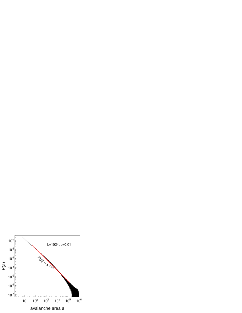
Figure 2: (Color online) The avalanche area distribution $P(a)$ does not follow exactly a power-law function. The parameters used in the numerical simulation were: density $c=0.01$ and linear lattice size $L=1024$.

For the two well known sandpile models, BTW ($c=0$) and Manna ($c=1$) the scaling exponents $\tau_{a,L\rightarrow\infty}(0)=1.26$, $\tau_{s,L\rightarrow\infty}(0)=1.23$, $\tau_{a,L\rightarrow\infty}(1)=1.36$, and $\tau_{s,L\rightarrow\infty}(1)=1.27$ were found. In addition, for all densities $c$ (see Fig. 1) the relation $\tau_{a,L\rightarrow\infty}(c)>\tau_{s,L\rightarrow\infty}(c)$ is valid.

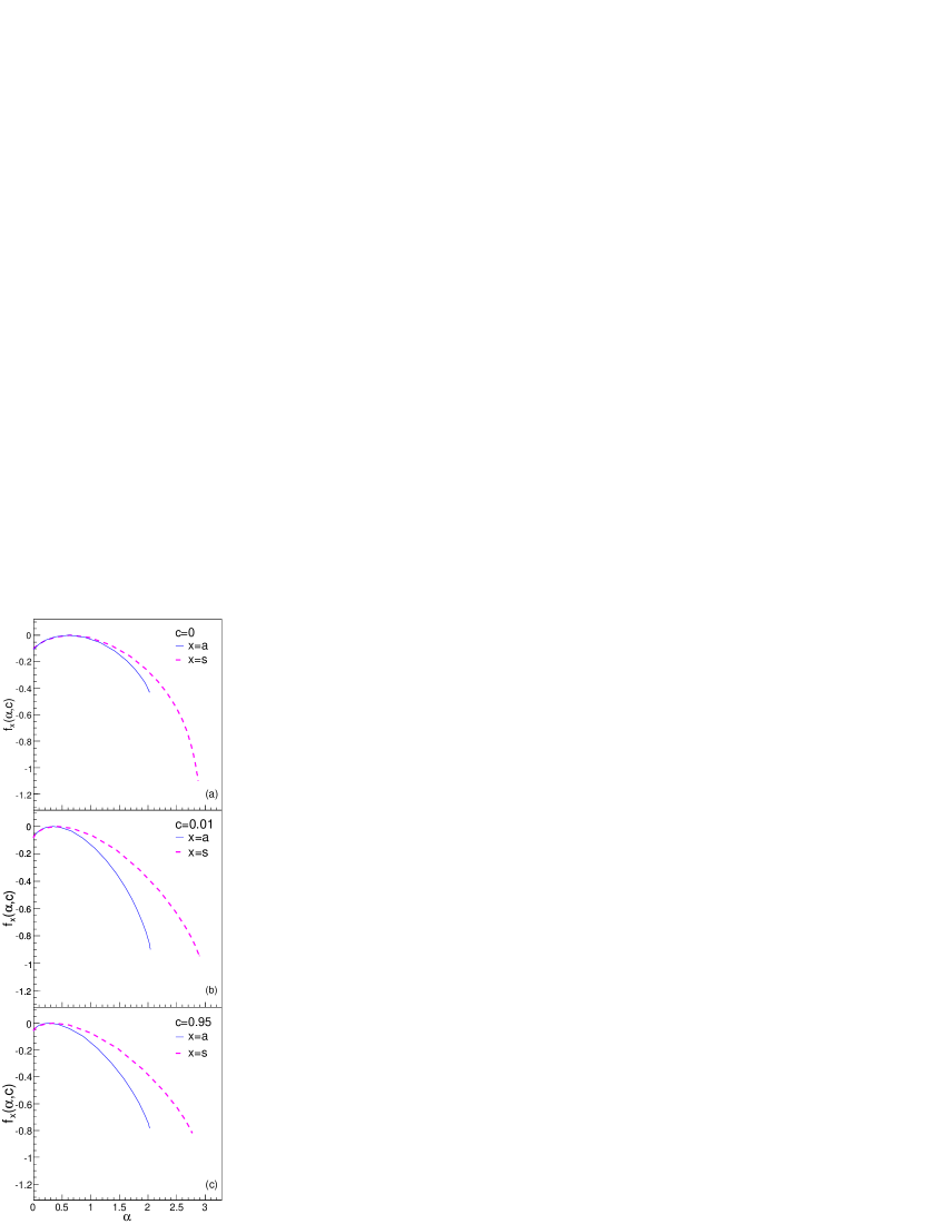
Figure 3: (Color online) The extrapolated spectra of the avalanche area $a$ and avalanche size $s$ for various densities of Manna toppling sites: (a) $c=0$ BTW model, which shows multifractal scaling, (b) $c=0.01$ at which the multifractal scaling of BTW model is destroyed, and (c) $c=0.95$ where the model shows the FSS near the two-state Manna model ($c=1$). The maximal error bars of $f(\alpha,c)$ are for $q\approx 0$, and are approximately $\pm 0.05$, but for a higher $q$ they are smaller. The $\alpha$ values are determined within errors $\pm 0.025$.

The scaling exponents $\tau_{x,L}$ as functions of the lattice size $L$ show a finite-size scaling effect [Eq. (7)]. An exact determination of scaling exponents $\tau_{x,L\rightarrow\infty}$ from numerical experiments is therefore a difficult task. A new method was introduced Lubeck to increase the numerical accuracy of the exponents based on their direct determination. We found that the method gives slightly larger exponents than a simple extrapolation of Eq. (7). However, the exponents $\tau_{s}$ do not fluctuate around their mean values as it was observed in the paper Lubeck . Our error bars were larger, therefore we have to repeat this analysis again in more details.

Tebaldi et al. Tebaldi_1999 found that in the BTW model the avalanche area distributions $P(a)$ show FSS and avalanche size distribution $P(s)$ scale as a multifractal. To describe these scaling properties rather a multifractal spectrum $f(\alpha)$ versus $\alpha$ than the single scaling exponent $\tau_{s}$ [Eq. (6)] is necessary. Thus, the scaling exponent $\tau_{s}$ loses the importance and is replaced by a spectrum of exponents. Despite this fact, the avalanche size scaling exponents $\tau_{s,L\rightarrow\infty}(0)$ are determined. They enable a comparison with the previous results, since the whole point is that the exponent $\tau_{s,L\rightarrow\infty}(0)$ does not exist. The recent studies Tebaldi_1999 ; Stella_2001 led us to analyze the multifractal properties of the model given by Eqs. (2)-(5) for various densities $c$. To determine the multifractal spectra a method presented in the paper Stella_2001 was useful. There, for any finite-size lattices $L$, the quantities $\alpha_{x}(q,L)=\left\langle log(x)x^{q}\right\rangle/\left[log(L)\left\langle x^{q}\right\rangle\right]$ and $\sigma_{x}(q,L)\sim log\left(\left\langle x^{q}\right\rangle\right)/log(L)$ were computed. It was observed that $\alpha_{x}(q,L)$ and $\sigma_{x}(q,L)$ show a finite-size dependence on the system size $L$, which is well approximated by Eq. (7) and this relation was used to extrapolate $L\rightarrow\infty$ quantities. Based on the Legendre structure relating $f_{x}$ to $\sigma_{x}$, a parametric representation of $f_{x}(\alpha_{x})$ by plotting $f_{x}(q)=\sigma_{x}(q)-\alpha_{x}(q)q$ versus $\alpha_{x}(q)$ can be obtained Stella_2001 .

Some significant spectra of $f_{x}(\alpha_{x},c)$ extrapolated for an infinite lattice size $L\rightarrow\infty$ are shown for illustration in Fig. 3. The $f_{x}(\alpha_{x},c)$ values were determined for the parameter $q$ in the range $-3.5<q<3.5$ and they are limited by errors about $\pm 0.08$, similarly as in Ref. Stella_2001 . We have observed that if $f_{x}(\alpha_{x},c)$ spectra are computed for all avalanches where $a>50$ then the errors of $f_{x}(\alpha_{x},c)$ are $\pm 0.05$. The multifractal scaling of the avalanche size probability distribution $P(s)$ and FSS of avalanche area probability distribution $P(a)$ were found at density $c=0$ (see Fig. 3 (a)). The avalanche probability distributions $P(x)$ show FSS for densities $c=0.01$ Fig. 3 (b), and for $c=0.95$ Fig. 3 (c) which is close to the Manna model ($c=1$). The spectra for $c=0$ and $1$ agree well with the previous results Stella_2001 . It was found that the multifractal scaling of $P(s)$ was destroyed (Fig. 3(b)) at a relatively small density of Manna sites $0<c<0.01$.

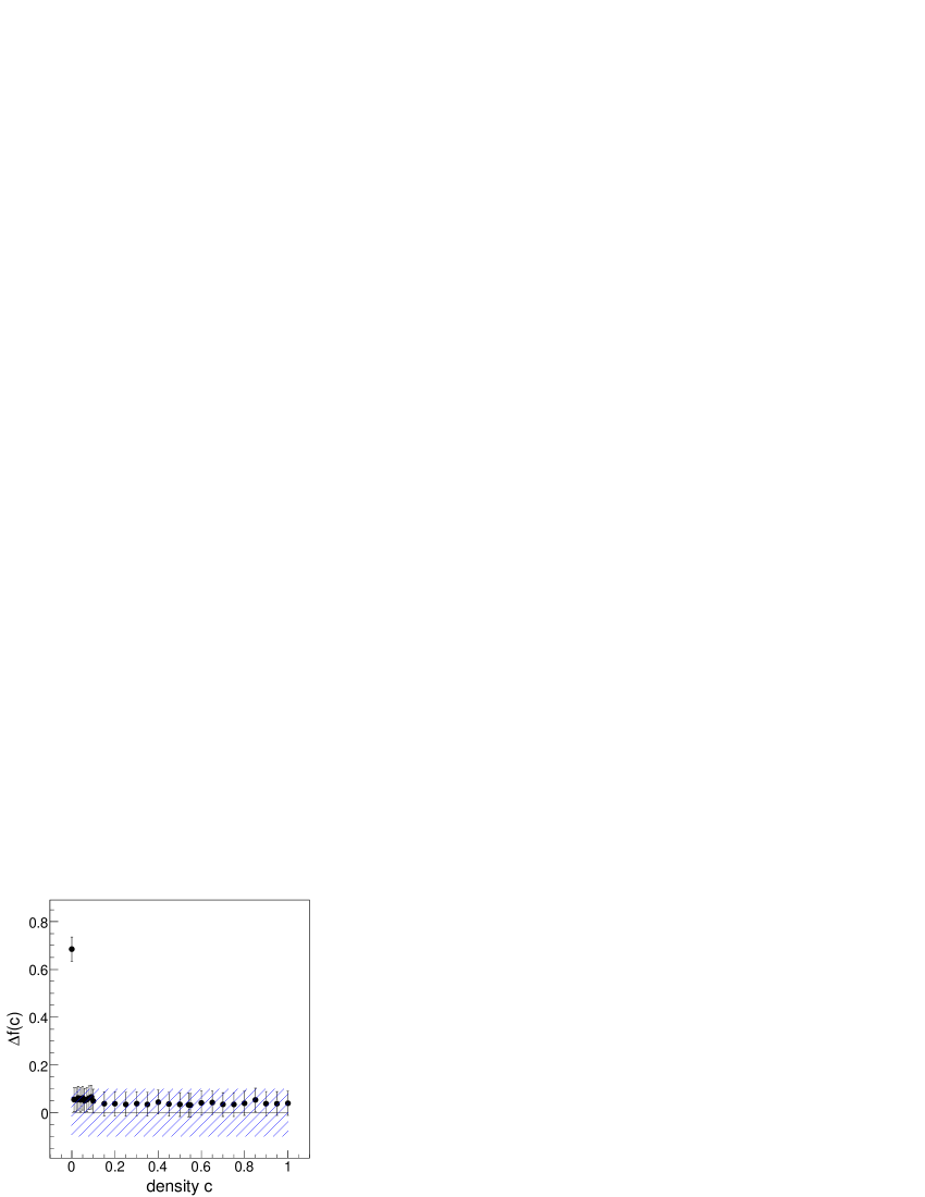
Figure 4: (Color online) A crossover from multifractal scaling to finite size scaling takes place at $0<c<0.01$. The hatched area border an interval of $\Delta f(c)$ in which $\Delta f(c)\doteq 0$ and probability distributions $P(x)$ show finite size scaling. We note that $\Delta f(c)=f_{a}^{min}(\alpha_{a},c)-f_{s}^{min}(\alpha_{s},c)$.

Stella et al. Stella_2001 claim that if probability distributions $P(x)$ satisfied FSS the large $q$ data accumulate in the same value $f_{x}(\alpha_{x})$ where $\alpha_{x}^{max}=D_{x}$ and $f_{x}=-(\tau_{x}-1)D_{x}$. However, for probability distribution showing the multifractal scaling there is no accumulation point and $f_{x}(\alpha_{x})$ points shift progressively down as the parameter $q$ is increasing and the parameter $q$ approaches $D_{x}$. This fact is utilized as a simple criterion to recognize which probability distributions show either multifractal scaling or FSS Stella_2001 . The equality $f_{a}^{min}(\alpha_{a},c)\doteq f_{s}^{min}(\alpha_{s},c)$ is considered to be an attribute that probability distributions $P(x)$ show FSS. To test this equality the differences $\Delta f(c)$ defined as $\Delta f(c)=f_{a}^{min}(\alpha_{a},c)-f_{s}^{min}(\alpha_{s},c)$ were determined. The equality $\Delta f(c)\doteq 0$ is considered for true if $\left|\Delta f(c)\right|\leq 0.10$ which reflects numerical errors. The differences $\Delta f(c)$ are shown in Fig. 4 where the hatched area limits the region where the equality is true and thus the avalanche probability distributions $P(x)$ show FSS behavior. It is clearly evident that only one value of $\Delta f(c)$ at the density $c=0$, is outside the region $\left|\Delta f(0)\right|>0.10$, and it corresponds to multifractal scaling of the BTW model Tebaldi_1999 ; Stella_2001 . We have no data from the interval of densities $0<c<0.01$ and thus we may only expect that a crossover from multifractal to FSS takes place in this interval.

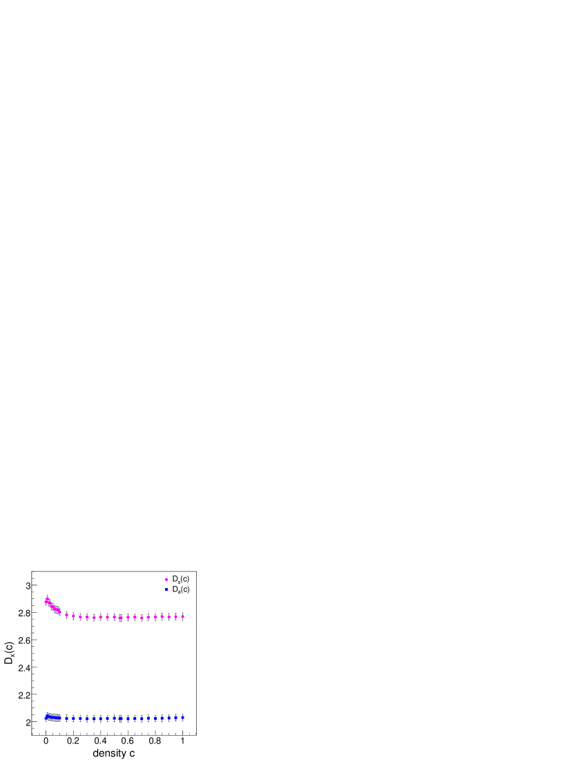
Figure 5: (Color online) The capacity fractal dimensions $D_{x=a,s}(c)$ as functions of the density $c$. The error bars are $\pm 0.025$.

The $f_{x}(\alpha_{x},c)$ spectra enable us to determine the capacity fractal dimensions $D_{x}(c)$ as $D_{x}(c)=\alpha_{x}^{max}(c)$. The results $D_{x}(c)$ for densities $0\leq c\leq 1$ are shown in the Fig. 5. For the BTW model $D_{s}(0)=2.88\pm 0.025$ and $D_{a}(0)=2.02\pm 0.025$, and for the Manna model $D_{s}(1)=2.77\pm 0.025$ and $D_{a}(1)=2.03\pm 0.025$ were found. The avalanche area capacity fractal dimensions $D_{a}(c)$ are almost constant $D_{a}(c)\doteq 2$, for any density $c$, and $D_{a}(0)\doteq D_{a}(1)$. In the interval of densities $0.01<c<0.15$ the avalanche size dimension $D_{s}(c)$ is decreasing from $D_{s}(0.01)=2.90$ to the value $D_{s}(0.15)=2.78$ and is then almost constant for $c>0.15$, finally $D_{s}(0)>D_{s}(1)$.

The moment analysis method Stella_2001 was used to clarify interesting properties of the scaling exponents $\tau_{x,L\rightarrow\infty}(c)$ which are shown in Fig. 1. The values of the functions $f_{x}^{min}(c)$ and $D_{x}(c)$ ( Fig. 5) are determined from the $f_{x}(\alpha_{x},c)$ plots. For specific densities $c=0$ (the BTW model) and $c=1$ (the Manna model) $f_{a}^{min}(0)=-0.43\pm 0.05$ and $f_{s}^{min}(1)=-0.784\pm 0.05$ were found. Then the scaling exponents are given $\tau_{x}(c)=1-f_{x}^{min}(c)/D_{x}(c)$ and are shown in the Fig. 6. For the density $c=0$, it was found $\tau_{a}(0)=1.213\pm 0.0125$. For the densities $0.01\leq c\leq 0.15$, the exponents decrease from $\tau_{a}(0.01)=1.441\pm 0.0125$ and $\tau_{s}(0.01)=1.329\pm 0.0125$ to the values $\tau_{a}(0.15)=1.394\pm 0.0125$ and $\tau_{s}(0.15)=1.299\pm 0.0125$, which are subsequently constant for $c>0.15$. For the density $c=1$, they are $\tau_{a}(1)=1.386\pm 0.0125$ and $\tau_{s}(1)=1.297\pm 0.0125$. These results are similar to those determined directly from the distribution functions $P(x)\sim x^{-\tau_{x}}$(Fig. 1).

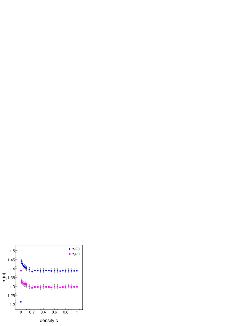
Figure 6: (Color online) The scaling exponents were determined using $\tau_{x}(c)=1-f_{x}^{min}(c)/D_{x}(c)$, for the moment analysis all avalanches where $a>50$ were taken into account.

IV Discussion

The plots of $\tau_{x,L}$ vs. $1/\ln L$ and an approximation given by Eq. (7) were used to extrapolate scaling exponents $\tau_{x,L\rightarrow\infty}$ Manna_PA ; Lubeck . Lübeck and Usadel Lubeck have analyzed an influence of an uncertainty in the determination of the exponents $\tau_{x,L}$ on the precision of the extrapolated exponents $\tau_{x,L\rightarrow\infty}$. Their results show that this method is not very accurate. However, this approximation enables us to make a comparison of our results with previous ones. The scaling exponents of the BTW model $\tau_{a,L\rightarrow\infty}(0)=1.26$ and $\tau_{s,L\rightarrow\infty}(0)=1.23$ (Fig. 1) are approximately the same as those found in Ref. Lubeck ($\tau_{a}=1.258$ and $\tau_{s}=1.247$) using the same method. The exponents of the Manna model $\tau_{a,L\rightarrow\infty}(1)=1.36$, and $\tau_{s,L\rightarrow\infty}(1)=1.27$ are comparable with the previous results, $\tau_{s,L=1024}=1.28\pm 0.02$ Manna_1991 and with $\tau_{a}=1.373$ and $\tau_{s}=1.275$, which were found by direct determination of exponents Lubeck or calculated from the moment analysis $\tau_{a}\doteq 1.36$ and $\tau_{s}\doteq 1.28$ Lubeck_2 . The results obtained by the moment analysis Stella_2001 , $f_{a}^{min}(0)=-0.43\pm 0.05$ and $f_{s}^{min}(1)=-0.784\pm 0.05$, agree well with the previous results, ${\textstyle\sigma_{a}=-0.391\pm 0.011}$ and $\sigma_{s}=-0.7900\pm 0.002$ Lubeck_2 . We may conclude that the experimental data for two known densities, $c=0$ and $1$, and data analysis methods give approximately the same exponents as were found in previous numerical experiments Manna_1991 ; Lubeck ; Lubeck_2 .

The scaling exponents defined by Eq. (6) Kadanoff and the conditional exponents $\gamma_{xy}$Christensen ; Ben-Hur can characterize the sandpile models. The theory predicts $\tau_{s}=1.253$ Pietronero and a few numerical experiments show $D_{s}\simeq 2.7$ and $D_{a}\simeq 2$ Pietronero ; Chessa . The conditional exponents $\gamma_{sa}$ determined directly from the numerical experiments are $\gamma_{sa}(0)=1.06$ and $\gamma_{sa}(1)=1.23$ Ben-Hur .

Let us assume that the BTW and Manna models belong to the same universality class. Then the scaling exponents $\tau_{x}(c),D_{x}(c)$ [Eq. (6] of the model (Eqs. (2)-(5)) must be independent on the density $c$, i.e. $\tau_{x}(c)=const.$ and $D_{x}(c)=const.$ This means that knowing only the scaling exponents ($\tau_{x}(c),D_{x}(c)$), we could not distinguish how many sites are toppling by deterministic or stochastic manner [Eq. (5)].

We observed that the capacity fractal dimensions $D_{a}(c)$ is constant for any density $c$, $D_{a}(c)\doteq 2$. The capacity fractal dimension $D_{s}(0)=2.88$ is the same as was found in the Ref. Stella_2001 , $D_{s}\doteq 2.86$ (determined from the Fig. 1(a) in Stella_2001 ). Our capacity fractal dimension $D_{s}(1)=2.77$ is higher than the value $D\simeq 2.7$ Manna_1991 ; Chessa , however it is closer to the $D\simeq 2.75$ Karma . In addition, for densities $0.01\leq c\leq 0.1$, the scaling exponents $\tau_{x,L\rightarrow\infty}(c)$, $\tau_{x}(c)$ (Figs. 1 and 6) and $D_{s}(c)$ (Fig. 5) depend on the density $c$. These scaling exponents and capacity fractal dimension are not constant. They demonstrate that the assumption about a single universality class is wrong and thus confirm the existence of different universality classes.

The conditional scaling exponents $\gamma_{xy}$ Christensen can be determined as $\gamma_{xy}(c)=(\tau_{y}(c)-1)/(\tau_{x}(c)-1)$ Lubeck_2 . Substituting the known scaling exponents $\tau_{x}(c)$ (Fig. 6), we determined $\gamma_{sa}(0.01)\doteq 1.34$ and for the Manna model, $\gamma_{sa}(1)\doteq 1.29$. We note that the scaling exponent $\tau_{s}(0)$ does not really exist.

To determine the exact scaling exponents of the probability distribution functions $P(x)$, the experimental data must show a power-law dependence given by Eq. (6). However, the avalanche area size distributions $P(a)$ do not follow exactly power-law distributions for densities $0<c\leq 0.1$ in the whole range of avalanche area sizes, a typical example is shown in the Fig. 2. Chessa et al. Chessa found that the area size distribution $P(a)$ of the BTW model ($c=0$) is not compatible with the FSS hypothesis in the whole range of avalanches. However, for large size of avalanches the FSS form must be approached. They assume that the scaling in the BTW model needs sub-dominant corrections of the form $P(x)=(C_{1}x^{-\tau_{1}}+C_{2}x^{-\tau_{2}}+\ldots)F(x/x_{c})$ where $C_{i}$ are nonuniversal constants and that these corrections do not determine universality class. The asymptotic scaling behavior is determined by the leading power law. We assume that the deviation from a simple power-law for densities $0<c\leq 0.1$ (Sec. III) could be explained by this correction. We observed that the exponents for large avalanches $a$ are larger than the approximate exponents ($\tau_{a,L=1024}=1.23$ in the Fig. 2) which cover the whole range. As a consequence, the leading exponents $\tau_{a,L}(c)$ for densities $0<c<0.1$ are higher than the approximate exponents which we found (they are not shown in the Fig.2 for $0<c\leq 0.09$). It is evident that the leading scaling exponents $\tau_{a,L}$ are different and are not constant (Fig. 1) as in the case of the BTW model or the Manna model and thus the model for these densities belongs to a different class than the BTW model or the Manna model.

Divergences from the expected power-law behaviour of the BTW model and a need of sub-dominant correction were observed in another inhomogeneous sandpile model Cer . Here the avalanche dynamic was disturbed by sites which had the second higher threshold. The effect was significant for thresholds $E_{C}\geq 32$ and low concentration of such sites Cer .

The multifractal properties (Fig. 3) of the model given by Eqs. (1)-(5) for the density $c=0$ (the BTW model), and FSS for the density $c=1$ (the Manna mode) agree well with the recent results Stella_2001 . In addition, the crossover from multifractal to FSS was observed in the Fig. 4. Our results can only predict that a critical density is expected to be found in the interval of densities $0<c<0.01$ (Figs. 3 and 4). This interval is five times smaller than what was found in Ref. Karma where the results are based on the autocorrelation function of the avalanche wave time series Menech_2 .

We assume that divergences from power-law dependences in inhomogeneous conservative models, Cer and Eqs. (1)-(5), have a common reason which is connected to the crossover from multifractal scaling to FSS Karma . In both models a disorder is induced by deployment of disturbing sites. These disturbing sites either increase the short range coupling during relaxations in deterministic model Cer or introduce the random toppling [Eq. (5)]. In these models toppling imbalance Karma_E ; Karma only for a few such sites can change character of waves in the models from coherent to more fragmented waves Ben-Hur ; Biham ; Milsh ; Stella_2001 .

In this study, the multifractal properties of the BTW model which is initially homogeneous, are destroyed at very low concentrations of such disturbing sites. In the opposite case, the Manna model shows the FSS and resistance to disturbance caused by presence of BTW sites because all significant exponents from Eq. (6) are approximately constant in a broad range of densities $0.15\leq c\leq 1$. One possible explanation for this is that the nature of the small perturbation of the model is not the same when we perform changes around the densities at $c=0$ and $c=1$. A small perturbation of the dynamical rules of the BTW model ($c=0$) breaks the toppling symmetry Karma and this may explain why the changes in the scaling exponents $\tau_{x}(c)$ and capacity fractal dimension $D_{s}(c)$ are so unexpected. On the other hand, for the Manna model ($c=1$), decreasing of the density $c$ cannot influence the unbalanced toppling symmetry of the Manna model Karma . For sandpile models which show FSS this is an expected result and agrees well with the theory Pietronero ; Chessa , where a small modification of toppling rules cannot change the scaling exponents.

We can clearly identify two universality classes which correspond to the classes proposed in papers Ben-Hur or Karma : (a) nondirected models, for density $c=0$ (BTW model, the multifractal scaling Tebaldi_1999 ; Stella_2001 ; Menech ), and they show a precise toppling balance Karma and they are sensitive on disturbance of avalanche dynamics, (b) random relaxation models, for densities $0.1<c<1$ where FSS of $P(x)$ is verified, they are nondirected only on average (Manna two-state model $c=1$ Ben-Hur ). In these models breaking of the precise toppling balance Karma is observed, the scaling exponents are resistant to disturbance of avalanches. The classification for densities $0<c<0.1$ is not so clear. If we follow the proposed classifications then the model is a random relaxation model Ben-Hur with broken precise toppling balance Karma and it belongs in the same class as the Manna model. On the other hand, the scaling exponents differ from the Manna model and they are not universal ($\tau_{x}(c)\neq const$., $D_{s}(c)\neq const.$), and the reasons of the sub-dominant approximation of area probability distribution functions Chessa can play an important role. We assume that a new universality class between the BTW ($c=0$, multifractal scaling) and the Manna ($c>0.5$, FSS) classes Karma ; Karma_E could be identified for densities $0<c<0.1$. However, a more detailed study is necessary to verify this classification.

Our additional arguments to the previous results Ben-Hur ; Biham ; Cer ; Karma ; Milsh ; Menech ; Lubeck show that small modifications of the dynamical rules of the model can lead to different universality classes what is considered to be unusual from a theoretical standpoint Chessa .

V Conclusion

In these computer simulations multifractal scaling of the BTW model Tebaldi_1999 and FSS of the Manna model Stella_2001 were confirmed. In addition, a crossover from multifractal scaling to FSS Karma was observed when avalanche dynamics of the BTW model was disturbed by Manna sites which were randomly deployed in the lattice, as their density was increased. This crossover takes place for a certain density $c$ in the interval $0<c<0.01$. This interval is five times smaller than what was found recently Karma . The scaling exponents $\tau_{x}(c)$ and the capacity fractal dimension $D_{s}(c)$ are not constant for all densities $c$ which is necessary if the models BTW_1987 ; Manna_1991 belong to the same universality class. These result agree well with the previous conclusions that multifractal properties of the BTW model Stella_2001 ; Tebaldi_1999 ; Menech , toppling wave character Ben-Hur ; Biham ; Milsh and precise toppling balance Karma ; Karma_E are important properties for solving the universality issues.

An open question remains about how to characterize the universality class for densities $0.01<c<0.1$, where the scaling exponents are not universal ($\tau_{x}(c)\neq const$. and $D_{s}(c)$$\neq const.$) and in addition, the avalanche probability distributions $P(a)$ do not show exact power-law behavior since the sub-dominant corrections of $P(a)$ Chessa are important. In this interval of densities $c$, our model belongs to the random relaxation models Ben-Hur and to the models with unbalanced toppling sites Karma ; Karma_E , however, its scaling exponents are not equal to the exponents of the Manna model.

Based on the previous findings Karma ; Karma_E and our results we assume that the avalanche dynamics of undirected conservative models, in which some of the probability distribution functions show a multifractal scaling (the BTW model), is disturbed by suitable toppling rules which are different from the two-state Manna model (for example a stochastic four-state Manna model Ben-Hur ; Milsh ), then a local manner for the energy distribution during the relaxation can be important and can change the scaling exponents. However, the models which show the FSS for all probability distribution functions (the Manna model) are not sensitive to the details of the toppling rules and are consistent with theoretical predictions Pietronero ; Chessa .

References

- (1) P. Bak, C. Tang, and K. Wiesenfeld, Phys. Rev. Lett. 59, 381 (1987); Phys. Rev. A 38, 364 (1988).
- (2) S. S. Manna, J. Phys. A 24, L363 (1991).
- (3) L. P. Kadanoff, S. R. Nagel, L. Wu and S. Zhou, Phys. Rev. A 39, 6524 (1989).
- (4) L. Pietronero, A. Vespignani, and S. Zapperi, Phys. Rev. Lett. 72, 1690 (1994); A. Vespignani, S. Zapperi, and L. Pietronero, Phys. Rev. E, 51, 1711 (1995).
- (5) M. De Menech, Phys. Rev. E 70, 028101 (2004).
- (6) S. Lübeck and K. D. Usadel, Phys. Rev. E 55, 4095 (1997).
- (7) A. Ben-Hur and O. Biham, Phys. Rev. E 53, R1317 (1996).
- (8) E. Milshtein, O. Biham, and S. Solomon, Phys. Rev. E 58, 303 (1998).
- (9) O. Biham, E. Milshtein, and O. Malcai, Phys. Rev. E 63, 061309 (2001).
- (10) A. Chessa, H. E. Stanley, A. Vespignani, and S. Zapperi, Phys. Rev. E 59, R12 (1999).
- (11) C. Tebaldi, M. De Menech and A. L. Stella, Phys. Rev. Lett. 83, 3952 (1999).
- (12) A. L. Stella and M. De Menech, Physica A 295, 101 (2001).
- (13) R. Karmakar, S. S. Manna, and A. L. Stella, Phys. Rev. Lett. 94, 088002 (2005).
- (14) R. Karmakar and S. S. Manna, Phys. Rev. E 71, 015101 (2005).
- (15) J. Černák, Phys. Rev. E 65, 046141 (2002).
- (16) D. Dhar, Physica A 263, 4 (1999).
- (17) S. S. Manna, Physica A 179, 249 (1991).
- (18) S. Lübeck, Phys. Rev. E 61, 204 (2000).
- (19) K. Christensen, H. C. Fogedby, and H. J. Jensen, J. Stat. Phys. 63, 653 (1991).
- (20) M. De Menech and A. L. Stella, Phys. Rev. E 62, R4528 (2000).
-
(21)
For more information see the web site
http://www.nordugrid.org