Roughness fluctuations, roughness exponents and the universality class of ballistic deposition

Abstract

In order to estimate roughness exponents of interface growth models, we propose the calculation of effective exponents from the roughness fluctuation $\sigma$ in the steady state. We compare the finite-size behavior of these exponents and the ones calculated from the average roughness $\langle w_{2}\rangle$ for two models in the $2+1$-dimensional Kardar-Parisi-Zhang (KPZ) class and for a model in the $1+1$-dimensional Villain-Lai-Das Sarma (VLDS) class. The values obtained from $\sigma$ provide consistent asymptotic estimates, eventually with smaller finite-size corrections. For the VLDS (nonlinear molecular beam epitaxy) class, we obtain $\alpha=0.93\pm 0.01$, improving previous estimates. We also apply this method to two versions of the ballistic deposition model in two-dimensional substrates, in order to clarify the controversy on its universality class raised by numerical results and a recent derivation of its continuous equation. Effective exponents calculated from $\sigma$ suggest that both versions are in the KPZ class. Additional support to this conclusion is obtained by a comparison of the full roughness distributions of those models and the distribution of other discrete KPZ models.

1 Introduction

Surface and interface growth processes attract much interest for their applications in solid state physics and material science [1, 2, 3]. They motivated the study of many interface growth models, which led to significant advances in non-equilibrium Statistical Mechanics and related fields [2, 3].

The simplest quantitative characteristic of a given interface is its roughness, also called the interface width, defined as the rms fluctuation of the height around its average position. The squared width, $w_{2}\equiv\overline{h^{2}}-{\overline{h}}^{2}$, is usually averaged over different configurations, and its scaling on time and length is used to characterize the growth process. For short times, in the so-called growth regime, the average roughness increases as ${\langle w_{2}\rangle}_{gr}\sim t^{2\beta}$, where $\beta$ is the growth exponent. For long times in a finite substrate, a steady state is attained, where the average roughness scales with the linear size $L$ as

$$\langle w_{2}\rangle\sim L^{2\alpha},$$ (1)

with $\alpha$ called the roughness exponent (notice that steady state averages are denoted without further labels here, while indexes $s$ or $sat$ are frequently used in the literature to denote saturation). The connection of discrete or continuous growth models to certain growth equations is frequently based on accurate numerical calculation of those scaling exponents. However, this procedure may be quite difficult when huge finite-size or finite-time corrections are present in the scaling of $\langle w_{2}\rangle$.

Alternatively, one may investigate features of the full roughness distribution, $P\left(w_{2}\right)$, which is the probability density of the roughness of a given configuration to lie in the range $\left[w_{2},w_{2}+dw_{2}\right]$. In recent years, the steady state distributions of several interface models have been analyzed [4, 5, 6, 7] and they were shown to fit the scaling form

$$P\left(w_{2}\right)={1\over\langle w_{2}\rangle}\Phi\left({w_{2}\over{\langle w_{2}\rangle}}\right).$$ (2)

Alternatively, the scaling relation

$$P\left(w_{2}\right)={1\over\sigma}\Psi\left({{w_{2}-\left<w_{2}\right>}\over\sigma}\right)$$ (3)

can be adopted, where

$$\sigma\equiv\sqrt{\left<{w_{2}}^{2}\right>-{\left<w_{2}\right>}^{2}}$$ (4)

is the rms deviation of the squared roughness. Despite the study of roughness distributions being useful for determining the universality classes of some growth processes, it is usually performed independently of the calculation of scaling exponents (notice that the values of the exponents are not necessary to fit the scaled distributions). Indeed, finite-size corrections in the universal functions $\Phi$ and $\Psi$ are typically much smaller than those in the Family-Vicsek scaling relation [8], which gives Eq. (1) a limiting case.

On the other hand, from Eqs. (3) and (4), we expect that the roughness fluctuation $\sigma$ in the steady state scales with exponent $\alpha$ as the average roughness:

$$\sigma\sim L^{2\alpha}.$$ (5)

Consequently, numerical estimates of $\sigma$ may also be used to estimate $\alpha$, but, as far as we know, this was not done in previous works. The expectation of weaker finite-size corrections using $\sigma$ instead of $\left<w_{2}\right>$ follows from the recent observation [7] that Eq. (3) provides a better data collapse of simulation data when compared to Eq. (2), for several growth models.

In order to estimate a scaling exponent with accuracy, the standard method is to extrapolate effective exponents obtained from consecutive slopes of log-log plots (see, e. g., Appendix A of Ref. [2]). Here, we will show that the effective exponents obtained from $\sigma$ provide reliable estimates of the roughness exponent and, in some cases, varies with $L$ slower than the estimates from the average width $\left<w_{2}\right>$. This is illustrated with applications to three growth models which belong to different universality classes, in one- and two-dimensional substrates.

Subsequently, we will apply this method to calculate the roughness exponent of two versions of the ballistic depositon (BD) model [9] in two-dimensional substrates. Numerical works showed discrepancies in the estimates of that exponent in $d=2$ and a rigorous derivation of a continuous equation for BD [10] deviates from the Kardar-Parisi-Zhang (KPZ) equation [12]. However, when effective exponents of BD are calculated with $\sigma$, the asymptotic estimates of $\alpha$ are close to the best known KPZ values. The conclusion that this is the universality class of BD is reinforced by the comparison of the full roughness distributions.

The rest of this work is organized as follows. In Sec. 2 we present the models which will be used to test the method for estimating roughness exponents and the results of these tests. In Sec. 3 we apply that method to two versions of BD in $d=2$ and analyze their roughness distributions. In Sec. 4 we summarize our results and conclusions.

2 Tests of the method in models of the KPZ and the VLDS classes

The first model analyzed here is the RSOS model [13], in which the incident particle can stick at the top of a column only if the differences of heights of all pairs of neighboring columns do not exceed ${\Delta H}_{max}=1$ after aggregation. Otherwise, the aggregation attempt is rejected. The second model was proposed for etching of a crystalline solid by Mello et al [14]: at each growth attempt, a randomly chosen column $i$, with current height $h(i)\equiv h_{0}$, has its height increased of one unit ($h(i)\rightarrow h_{0}+1$), and all neighboring column whose heights are smaller than $h_{0}$ grows to $h_{0}$ (this may be called the growth version of the etching model [11]).

In the limit of large lengths and long times, these models are represented by the KPZ equation [12]

$${{\partial h}\over{\partial t}}=\nu_{2}{\nabla}^{2}h+\lambda_{2}{\left(\nabla h\right)}^{2}+\eta(\vec{x},t).$$ (6)

Here, $\nu_{2}$ and $\lambda_{2}$ are constants and $\eta$ is a Gaussian noise with zero mean and variance $\langle\eta\left(\vec{x},t\right)\eta\left(\vec{x^{\prime}},t^{\prime}\right)\rangle=D\delta^{d}\left(\vec{x}-\vec{x^{\prime}}\right)\delta\left(t-t^{\prime}\right)$, where $d$ is the dimension of the substrate. In $d=1$, the exact roughness exponent is $\alpha=1/2$ [12, 2], and in $d=2$ the best numerical estimates are around $0.38-0.39$ [15, 11]. Numerical estimates of $\left<w_{2}\right>$ for the RSOS and etching models in $d=1$ provide estimates of exponents which converge to the exact values with negligible finite-size corrections. However, that is not the case in $d=2$, particularly for the etching model [11], consequently our tests will focus this case.

The widths $\left<w_{2}\right>$ and their fluctuations $\sigma$ were calculated at the steady states in two-dimensional substrates up to $L=256$ for the RSOS model and up to $L=512$ for the etching model. Finite-size estimates of the roughness exponents are given by

$$\alpha_{w}\left(L\right)\equiv{1\over 2}{\ln{\left[{\langle w_{2}\rangle}\left(L\right)/{\langle w_{2}\rangle}\left(L/2\right)\right]}\over\ln{2}}$$ (7)

and

$$\alpha_{\sigma}\left(L\right)\equiv{1\over 2}{\ln{\left[\sigma\left(L\right)/\sigma\left(L/2\right)\right]}\over\ln{2}}.$$ (8)

The presence of significant corrections to Eqs. (1) and (5) is reflected in a size-dependence of $\alpha_{w}\left(L\right)$ and $\alpha_{\sigma}\left(L\right)$. These effective exponents are shown in Fig. 1 for the RSOS and the etching models as a function of $1/L$ and $2/L$, respectively.

An asymptotic estimate near $0.39$ is consistent with the trend of the RSOS data as $L\to\infty$. For this model, small differences in the estimates obtained from $\left<w_{2}\right>$ and $\sigma$ are observed, as well as weak finite-size effects. The linear fit of $\alpha_{w}\left(L\right)$ shown in Fig. 1 suggests $\alpha\approx 0.39$.

However, the finite-size dependence of the data for the etching model is remarkable: the effective exponents vary between $0.34$ and $0.38$ in Fig. 1. For the largest lengths $L$, $\alpha_{\sigma}\left(L\right)$ approaches the asymptotic region $\alpha\approx 0.39$ faster than $\alpha_{w}\left(L\right)$, as illustrated by the curves through the data points in Fig. 1. It suggests that, for large $L$, the corrections to the scaling of $\sigma$ are smaller than the corrections to $\left<w_{2}\right>$. Although the fits of the data in Fig. 1 do not represent systematic extrapolation procedures, our interpretation is reinforced by the fact that the extrapolated $\alpha_{\sigma}\left(L\right)$ for the etching model is very close to the value predicted by the RSOS model.

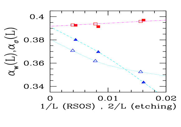
Figure 1: Effective exponents $\alpha_{w}\left(L\right)$ (empty symbols) and $\alpha_{\sigma}\left(L\right)$ (full symbols), for the RSOS model (squares) and the etching model (triangles) in two-dimensional substrates, as a function of $1/L$ or $2/L$. $\alpha_{\sigma}\left(L\right)$ data are slightly shifted to the right to avoid superposition of data points. Error bars are compared to the size of the points, except for the largest lengths, in which the uncertainties are around $0.005$ for both models. The lines connecting the data points (except $\alpha_{\sigma}\left(L\right)$ data for the RSOS model) were drawn to guide the eye.

For the etching model, we were not able to perform reliable extrapolations of $\alpha_{w}\left(L\right)$ or $\alpha_{\sigma}\left(L\right)$ as functions of $1/L^{\Delta}$, with any exponent $\Delta>0$ (the value $\Delta=1$ is used in Fig. 1). This is related to the large deviations from the asymptotic scaling in small lattices, typically $L<50$. It contrasts to Ref. [11], where a extrapolation of $\alpha_{w}\left(L\right)$ up to $L=1024$ was possible with $\Delta\sim 0.5$. However, here we are working with data for $L\leq 256$ because there are very large error bars in the estimates of $\sigma$ for larger lattices. With a small number of data points, even more sophisticated extrapolation methods [16] are not able to provide better estimates than previous work.

An extended version of the conserved RSOS (CRSOS) model is also suitable for this test. In this model, if the aggregation at the column of incidence disobeys the condition ${\Delta H}_{max}=1$, then the incident particle executes a random walk among neighboring columns until finding a column in which it can aggregate [17]. The CRSOS model belongs to the class of the nonlinear molecular-beam epitaxy equation, or Villain-Lai-Das Sarma (VLDS) equation [18, 19]

$${{\partial h}\over{\partial t}}=\nu_{4}{\nabla}^{4}h+\lambda_{4}{\nabla}^{2}{\left(\nabla h\right)}^{2}+\eta(\vec{x},t),$$ (9)

where $\nu_{4}$ and $\lambda_{4}$ are constants. Our extended version of the CRSOS model is different from the original one [20] but has the same symmetries and, consequently, belong to the same universality class.

In Fig. 2 we show the effective exponents of this model obtained from simulations up to $L=256$, with linear fits of both data sets. The evolution of $\alpha_{\sigma}\left(L\right)$ and $\alpha_{w}\left(L\right)$ suggest $\alpha\approx 0.93$ asymptotically, but the difference between $\alpha_{\sigma}\left(L\right)$ and the asymptotic value is clearly much smaller. This is consistent with the different slopes of the linear fits shown in Fig. 2 (smaller slope for fitting $\alpha_{\sigma}\left(L\right)$).

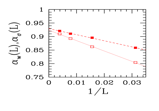
Figure 2: Effective exponents $\alpha_{w}\left(L\right)$ (empty squares) and $\alpha_{\sigma}\left(L\right)$ (full squares), for the CRSOS model in one-dimensional substrates, as a function of $1/L$. Error bars are of the size of the data points. The dotted and dashed lines are linear fits of each data set.

This application provides additional support to the conclusion that $\alpha<1$ in the VLDS class in $d=1$ [21] ($\alpha=1$ is obtained from one-loop renormalization). The estimate $\alpha=0.93\pm 0.01$ follows from the extrapolation of those data. It improves our previous estimate $\alpha=0.94\pm 0.02$, obtained in Ref. [17], where effective exponents were calculated from the second and fourth moments of the height distribution in sizes up to $L=1024$.

The above analysis, performed with models in different universality classes and with noticeable (but not huge) finite-size corrections to Eq. (1), shows that roughness exponents may be estimated from $\sigma$ with comparable or higher accuracy than those obtained from $w_{2}$, suggesting its application to controversial situations.

3 Application to ballistic deposition

In the simplest version of the ballistic deposition model, particles are released from a randomly chosen position above a $d$-dimensional substrate, follow trajectories perpendicular to the surface and stick upon first contact with a nearest neighbor occupied site [8, 9]. The resulting aggregate is porous and has a rough surface. Several applications of the BD model or its extensions to real growth processes were already proposed, which justifies the present analysis (see e. g. recent applications in Refs. [22, 23]).

The mechanism of lateral aggregation suggests that BD is in the KPZ class. However, several numerical works on this model showed discrepancies between the estimated exponents and the KPZ values [8, 24, 25, 26]. In a recent work, we have shown that the KPZ values are obtained with good accuracy in $d=1$ if effective exponents $\alpha_{w}\left(L\right)$ are properly extrapolated [27]. In $d=2$, the effective roughness exponents rapidly vary with $L$, but they are still far from the region $[0.38,0.40]$ up to $L=512$ [27]. An apparent consistency with the KPZ value is obtained in $d=2$ only after assuming of a constant correction term in Eq. (1) (the intrinsic width), but error bars are very large [11]. Consequently, from numerical work, there is no clear evidence that BD is in the KPZ class in $d=2$.

Recently, Katzav and Schwartz derived a continuous equation for another version of BD which differs from the KPZ equation [10]. They analyzed the BD model with next-nearest neighbor aggregation, hereafter called BDNNN, in which the incident particle sticks upon first contact with a nearest neighbor or with a next-nearest neighbor occupied site. In $d=1$, they showed that the squared gradient in Eq. (6) is replaced by the absolute value of the gradient in the continuous equation corresponding to BDNNN. This is suggested as a possible reason for the slow convergence of the scaling exponents to their asymptotic values. In $d\geq 2$ the situation is more complicated: the only contribution to the local growth rate comes from the direction $x_{m}$ along which the height gradient is maximum, and that contribution is ${1\over 2}{{\partial^{2}h}\over{\partial{x_{m}}^{2}}}+\left|{{\partial h}\over{\partial x_{m}}}\right|$. This accounts for the maximal growth ingredient of the model. However, the presence of the lattice axis in that equation contrasts with the rotation symmetry of the KPZ equation. Thus, also from analytical work, there is no a priori reason to expect BD to be in the KPZ class [10].

This scenario motivates the extension of our method to estimate roughness exponents of BD and BDNNN in $d=2$. Simulations of both models were performed in lattices up to $L=512$, where $w_{2}$ and $\sigma$ can be obtained with reasonable accuracy. The number of different realizations used to estimate those quantities were near ${10}^{8}$ for $L\leq 128$, ${10}^{7}$ for $L=256$ and $2\times{10}^{6}$ for $L=512$.

In Fig. 3a we show $\alpha_{w}\left(L\right)$ and $\alpha_{\sigma}\left(L\right)$ for the original BD model. $\alpha_{w}\left(L\right)$ rapidly varies with $L$ in the whole range of our data and attains a value near $0.28$ in the largest lattice, which is much smaller than the estimates for the KPZ class. This complex finite-size behavior was already pointed out in Ref. [27] and, consequently, no reliable extrapolation of $\alpha$ could be extracted from those data. On the other hand, $\alpha_{\sigma}\left(L\right)$ is in the range $[0.36,0.37]$ for the largest $L$. As $1/L\to 0$, Fig. 3a indicates that $\alpha_{\sigma}\left(L\right)$ converges to an asymptotic value between $0.36$ and $0.4$.

In Fig. 3b we show the effective exponents for the BDNNN model. We notice that $\alpha_{w}\left(L\right)$ is even farther from the KPZ estimate in this model. However, the trend of $\alpha_{\sigma}\left(L\right)$ as $1/L\to 0$ suggests an asymptotic value between $0.35$ and $0.4$, although finite-size effects seem to be much stronger than those of the original BD model.

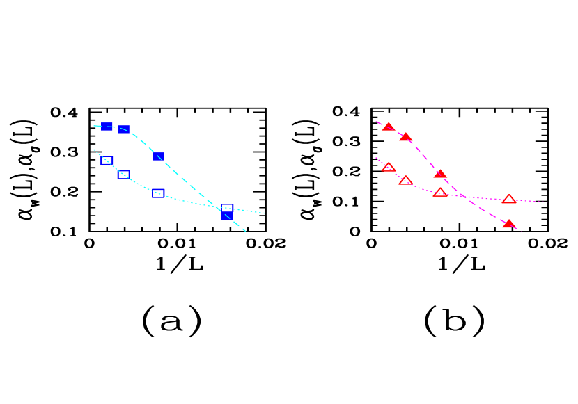
Figure 3: Effective exponents $\alpha_{w}\left(L\right)$ (empty symbols) and $\alpha_{\sigma}\left(L\right)$ (full symbols) for: (a) the original BD model in $d=2$; (b) the BDNNN model in $d=2$. The lines connecting the data points were drawn to guide the eye.

Extrapolations of $\alpha_{w}\left(L\right)$ and $\alpha_{\sigma}\left(L\right)$ for BD and BDNNN as functions of $1/L^{\Delta}$, varying the exponent $\Delta$ along the same lines of Ref. [11], were also tested, but no significant improvement of the above mentioned estimates was obtained. However, those estimates are consistent with the best currently avaiable values for the KPZ class, which lie in the range $\left[0.375,0.396\right]$ [15, 11], which strongly suggests that BD and BDNNN are also in that class in $d=2$.

Another important test is a comparison of the full roughness distributions of these models and that of other KPZ models. The distribution for the RSOS model, which shows negligible finite-size effects, can be used as a representative of the KPZ class [7]. In Fig. 4 we show this distribution, scaled according to Eq. (3), and the scaled distributions for the BD and the BDNNN models in $L=256$ (data for $L=512$ was not used here due to their lower accuracy, mainly in the tails of the distribution). The collapse of all data into a single universal curve reinforces our conclusion that both models are in the KPZ class in $d=2$.

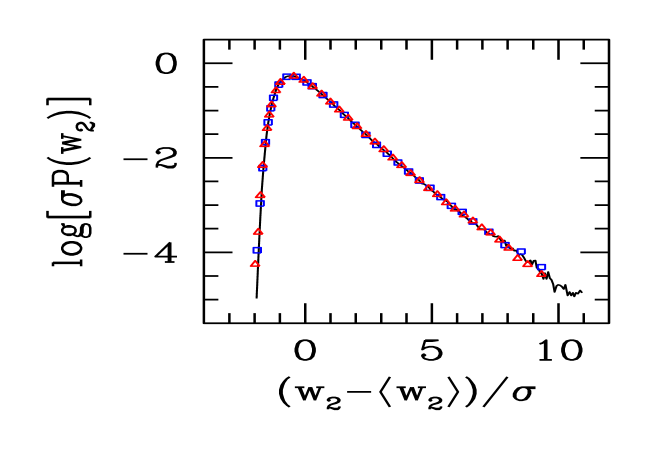
Figure 4: Scaled roughness distribution at the steady states of the RSOS model (solid curve), the BD model (squares) and the BDNNN model (triangles), in $2+1$-dimensional lattices of length $L=256$.

A quantitative support to the universality of the scaled distributions of Fig. 4 is given by the estimates of the skewness and kurtosis of those curves. For the RSOS and the etching models, $S=1.70\pm 0.02$ and $Q=5.4\pm 0.3$ were obtained in Ref. [7]. Here, for BD we obtained $S=1.71\pm 0.02$ and $Q=5.4\pm 0.1$, and for BDNNN we obtained $S=1.67\pm 0.03$ and $Q=5.2\pm 0.3$, both in good agreement with the values of the other KPZ models.

4 Conclusion

We proposed the calculation of roughness exponents from the scaling of roughness fluctuations $\sigma$ in the steady states. Tests for two models in the $2+1$-dimensional KPZ class and for a model in the $1+1$-dimensional VLDS class were performed and showed that effective exponents obtained from that quantity provide comparable or better asymptotic estimates than the average width $\langle w_{2}\rangle$. We also applied this method to two versions of the ballistic deposition model, the original one (BD) and the next-nearest neighbor one (BDNNN), in order to clarify a controversy on its universality class raised by numerical results and an exact derivation of its corresponding continuous equation. Effective exponents calculated from $\sigma$ suggest that the asymptotic class is KPZ, while those calculated from $\langle w_{2}\rangle$ show much more complex finite-size behavior. Additional support to this conclusion is obtained from the collapse of the full roughness distributions of those models into the distribution of the RSOS model.

At this point it is important to recall that higher moments of the height distribution, such as the fourth moment $\left<w_{4}\right>\equiv\left<\overline{{h-\overline{h}}^{4}}\right>$, are also frequently used to estimate the roughness exponent. Their accuracy is usually lower than that of $\left<w_{2}\right>$ and, consequently, do not improve the estimates of $\alpha$ (see e. g. Ref. [11]). This quantity, however, must not be confused with $\sigma^{2}$, which is the fluctuation of the global roughness in the steady state.

The successful application of the above method to estimate the roughness exponent, possibly combined with the analysis of roughness distributions, suggests its extension to other models in which remarkable finite-size corrections in the effective exponents are observed.

References

- [1] Frontiers in surface and interface science, eds. C.B. Duke, E. W. Plummer, Elsevier Science B.V., Holanda (2002) .
- [2] A.L. Barabási and H.E. Stanley, Fractal concepts in surface growth (Cambridge University Press, Cambribge, England, 1995).
- [3] J. Krug, Adv. Phys. 46, 139 (1997).
- [4] G. Foltin, K. Oerding, Z. Rácz, R. L. Workman, and R. K. P. Zia, Phys. Rev. E 50 (1994) R639.
- [5] Z. Rácz and M. Plischke, Phys. Rev. E 50 (1994) 3530.
- [6] T. Antal, M. Droz, G. Györgyi, and Z. Rácz, Phys. Rev. E 65 (2002) 046140.
- [7] F. D. A. Aarão Reis, Phys. Rev. E (2005) accepted for publication.
- [8] F. Family and T. Vicsek, J. Phys. A 18 (1985) L75.
- [9] M. J. Vold, J. Coll. Sci. 14 (1959) 168; J. Phys. Chem. 63 (1959) 1608.
- [10] E. Katzav and M. Schwartz, Phys. Rev. E 70 (2004) 061608.
- [11] F. D. A. Aarão Reis, Phys. Rev. E 69 (2004) 021610.
- [12] M. Kardar, G. Parisi and Y.-C. Zhang, Phys. Rev. Lett. 56 (1986) 889.
- [13] J. M. Kim and J. M. Kosterlitz, Phys. Rev. Lett. 62 (1989) 2289.
- [14] B. A. Mello, A. S. Chaves and F. A. Oliveira, Phys. Rev. E 63 (2001) 41113.
- [15] E. Marinari, A. Pagnani and G. Parisi, J. Phys. A 33 (2000) 8181.
- [16] M. Henkel and G. M. Schutz, J. Phys. A 21 (1988) 2617.
- [17] F. D. A. Aarão Reis and D. F. Franceschini, Phys. Rev. E 61 (2000) 3417; F. D. A. Aarão Reis, Phys. Rev. E 70 (2004) 031607.
- [18] J. Villain, J. Phys. I 1 (1991) 19.
- [19] Z.-W. Lai and S. Das Sarma, Phys. Rev. Lett. 66 (1991) 2348.
- [20] Y. Kim, D. K. Park and J. M. Kim, J. Phys. A 27 (1994) L533.
- [21] H. K. Janssen, Phys. Rev. Lett. 78 (1997) 1082.
- [22] K. Trojan and M. Ausloos, Physica A 326 (2003) 492.
- [23] M. Grzegorczyk, M. Rybaczuk, and K. Maruszewski, Chaos, Solitons and Fractals 19 (2004) 1003.
- [24] P. Meakin, P. Ramanlal, L. M. Sander and R. C. Ball, Phys. Rev. A 34 (1986) 5091.
- [25] R. M. D’Souza, Int. J. Mod. Phys. C 8 (1997) 941.
- [26] R. Miranda, M. Ramos, and A. Cadilhe, Comput. Mater. Sci. 27 (2003) 224.
- [27] F. D. A. Aarão Reis, Phys. Rev. E 63 (2001) 056116.