Unified Multifractal Description of Velocity Increments Statistics in Turbulence: Intermittency and Skewness
Abstract
The phenomenology of velocity statistics in turbulent flows, up to now, relates to different models dealing with either signed or unsigned longitudinal velocity increments, with either inertial or dissipative fluctuations. In this paper, we are concerned with the complete probability density function (PDF) of signed longitudinal increments at all scales. First, we focus on the symmetric part of the PDFs, taking into account the observed departure from scale invariance induced by dissipation effects. The analysis is then extended to the asymmetric part of the PDFs, with the specific goal to predict the skewness of the velocity derivatives. It opens the route to the complete description of all measurable quantities, for any Reynolds number, and various experimental conditions. This description is based on a single universal parameter function and a universal constant .
keywords:
Isotropic turbulence , Intermittency , Skewness , Longitudinal velocity statistics , Multifractal formalismPACS:
02.50.Fz , 47.53.+n , 47.27.Gs,
1 Introduction
In the field of turbulence, a significant effort has been devoted to the analysis of the scaling behavior of structure functions , where is the longitudinal velocity increment between two points separated by a variable distance [1]. However, a better strategy may be to concentrate on the probability density functions (PDFs) of , rather than on a set of moments [2]. Accordingly, this work deals with the description of the PDFs of , where the scale spans the entire range of excited scales of motion (from the integral far down to the dissipative scales). Experimental and numerical observations have provided the evidence that the PDFs of are increasingly stretched as decreases, while they are almost Gaussian at the large scales where the turbulence is stired [1]. This feature is known as intermittency. Moreover, Chevillard et al. [3] have recently argued that this stretching is largely enhanced in the near-dissipation range, leading to extremely high fluctuation level for the velocity gradients. Another essential feature lies in the significant asymmetry, or skewness, of the PDFs. This skewness to be non-zero is heuristically connected to the vortex folding and stretching (irreversible) process, which drains energy from the large to the small scales, and hence, plays a central role in turbulence. From a theoretical viewpoint, a quantitative description of the skewness is still missing. In this context, our motivation is to present a synthetic description of the PDFs of , which encompasses the combined effects of intermittency and skewness. To do so, the PDF of is split into a symmetric and an asymmetric part. First, the focus is on , which also represents the PDF of the magnitude of . We show that is suitably described by a multifractal picture of turbulence dynamics [1], which incorporates finite-Reynolds-number effects. The analysis is then extended to with the specific goal to describe the skewness phenomenon via a quantitative estimate of the skewness factor as a function of .
2 Statistics of longitudinal velocity increment magnitude: Modeling the symmetric part of the Probability Density Function
From a general point of view, the PDF of the longitudinal velocity increments can be split into a symmetric (i.e. even) function and an asymmetric (i.e. odd) function in the following way:
| (1) |
The PDF of the longitudinal velocity increment magnitude shows that the symmetric part of the PDF of describes the magnitude statistics. Notice that neither nor can be interpreted as a PDF of a random variable.
Let us first focus on the symmetric part of the PDFs of the longitudinal velocity increments . In the inertial range, the multifractal formalism [4], which a priori pertains in the limit of infinite Reynolds number, states that velocity is everywhere singular, the longitudinal velocity increments at scale behaving locally as , where the Hlder exponent takes value in a finite interval . When the Reynolds number is finite ( is the correlation length scale, and the kinematic viscosity), Paladin and Vulpiani [5] have argued that the dissipative scale, that is supposed to separate the inertial and the dissipation scaling ranges, is not unique in the presence of intermittency and is likely to depend on . Using these arguments, Nelkin [6] predicted the moments of velocity gradients, i.e. . The phenomenological consequences on the energy power spectrum were studied by Frisch and Vergassola [7] who proved the existence of an intermediate dissipative range. Meneveau [8] further investigated the behavior of the structure functions in that transitory range. Recently, Chevillard et al. [3] revisited the behavior of longitudinal velocity increments in the intermediate dissipative range and showed, among other new predictions, that the width of this range of scales behaves non trivially with the Reynolds number, i.e. .
To provide a complete statistical description of longitudinal velocity increments statistics, one needs to model the probability law of the stochastic variable . As originally proposed by Castaing et al. [9], within the propagator approach, velocity increments magnitude can be considered as the product of two independent random variables, (in law), where is a zero-mean gaussian random variable of variance and a positive random variable (see [3] for details). In the inertial range, i.e. , where is the fluctuating dissipative scale, can be expressed as a function of the singularity strength that fluctuates from point to point according to the probability law . Note that the exponent and the parameter function gain the mathematical status of Hlder exponent and singularity spectrum in the inviscid limit (). The dissipative scale fluctuates according to : , where the constant is necessary to be consistent with experimental and numerical data [10, 11, 12]. More precisely, in a monofractal description of velocity fluctuations (Kolmogorov K41 theory [1]), one can show [3] that the Kolmogorov constant . Actually in this simplified monofractal framework, the average local dissipation can be related to the ratio (where is the Taylor based Reynolds number). We will see in the following that the data are compatible with the universal value (in the presence of intermittency).
For scales , the velocity is smooth and Taylor’s development applies, i.e. . In the multifractal description, using a simple continuity argument with the inertial range behavior [6] yields and . Then, we impose that the function be continuous and differentiable at the transition, following a strategy already used in a slightly different form in Ref. [8], and which is inspired from an elegant interpolation formula originally proposed by Batchelor [13], independently derived in a field theoretic approach [14]. In this framework, a single function covers the entire range of scale:
| (2) |
and
| (3) |
where is a normalization factor such that .
From Eqs. (2) and (3), one can derive analytical predictions for the moments of the longitudinal velocity increment modulus, i.e. , the energy power spectrum (which is linked to the Fourier transform of the second order moment [15, 16]) and the symmetric part of the longitudinal velocity increments PDF. This approach has also been successfully applied in the Lagrangian framework in which the PDFs are symmetric [17, 18].
As advocated in Ref. [19], the magnitude cumulant analysis provides a more reliable alternative to the structure function method. The relationship between the moments of and the cumulants of reads
| (4) |
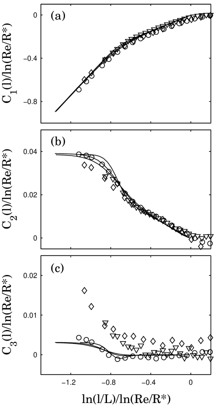
In Fig. 1, we report the results of the computation of the magnitude cumulants of various experimental velocity signals. Actually we have plotted the cumulants of instead of , so that they vanish at the correlation length scale (as the signature of Gaussian statistics). When both the cumulants and are renormalized by , all the curves collapse on a universal linear function in the inertial range (when , see [3]) of slope . Let us notice that in this representation, for any Reynolds number, and , where and are respectively the Kolmogorov and the Taylor scales. For the first order cumulant (Fig. 1(a)), disregarding large scale anisotropy leading to nonuniversal effects, is found very close to , consistently with K41 theory [1]. For the second-order cumulant (Fig. 1(b)), the intermittency coefficient is found universal, i.e. independent of the Reynolds number and of the experimental configuration. For the third one, cannot be claimed to be different from zero (especially at high Reynolds number) confirming that the statistics of longitudinal velocity increments are likely to be log-normal [19, 23]. In the intermediate dissipative range (i.e. ), crosses over towards trivial scaling; the straight line of slope unity observed at smaller scales means that velocity increments become proportional to the scale (Taylor development). The behavior of the second-order cumulant is much more interesting and has been widely studied in Ref. [3] : a non trivial Reynolds dependent rapid increase occurs in the intermediate dissipative range, the larger the Reynolds number, the more “rapid” the increase. Finally, tends toward a universal value in the far-dissipative range. Note that displays similar behavior. In Fig. 1 are also represented our theoretical predictions obtained from the computation of the moments of using Eqs. (2) and (3), i.e. . We have used the following set of parameters: and a universal log-normal parabolic function,
| (5) |
with and to ensure that in the inviscid limit [1]. The integration limits and are respectively the minimal and maximal values such that . Using Eq. (5), we get and . The different curves so-obtained superimpose remarkably well with the corresponding data for the first two cumulants which demonstrates that our multifractal description accounts quantitatively well for the departure from scaling in the intermediate dissipative range. Finite Reynolds number effects [23], statistical convergence and lognormal approximation can explain some discrepancies between our theoretical prediction and the behavior of the third-order cumulant.
3 Multifractal prediction of the skewness of longitudinal velocity increments
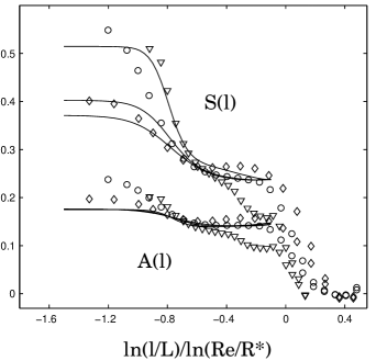
Let us now investigate the statistics of signed longitudinal velocity increments through the two estimators: (i) the skewness and (ii) the asymmetry factor . The experimental estimates of and are shown in Fig. 2 in a semi-logarithmic representation. Interestingly, displays a plateau at about 0.14 in the inertial range, whereas the skewness behaves approximatively as a power law. In the intermediate dissipative range, both estimators undergo a rapid acceleration, very much like what was observed for in Fig. 1(b). From a theoretical point of view, the third-order structure function is solution of the Kármán-Howarth-Kolmogorov equation [24]
| (6) |
This equation allows us to compute the third-order structure function when the second-order one and the average local dissipation are known. A similar approach has been performed by Qian in Ref. [25] without taking into account the intermittency corrections.
We have superimposed in Fig. 2 our theoretical predictions to the experimental data for and . Indeed, from Eqs. (2) and (3), one can compute any moment of the magnitude of velocity increments and velocity gradient . In particular, we get
| (7) |
where is the limit when of the normalization factor appearing in Eq. (3). Then, by inserting our description of the second order structure function (Eq. (4) for ) together with the prediction of the average local dissipation (Eq. (7)) in Eq. (6), we get the third order moment of velocity increments at any scale and Reynolds number. As shown in Fig. 2, the agreement is very good for distances in between the Kolmogorov and Taylor scales (without any arbitrary shifts) when using the same parameter function and as in our former magnitude cumulant analysis.
Furthermore, we can derive that, when neglecting intermittency corrections and setting the viscosity to zero in Eq. (6), we get and , in perfect agreement with experimental findings. Some discrepancies occur for , especially for Modane’s longitudinal velocity profile, because (i) of the lack of statistics and (ii) at these scales, one has to take into account in Eq. (6) fluctuations of the injection rate of energy [26, 27]. In the intermediate and far dissipative range, our formalism predicts a universal plateau and a Reynolds number dependence for respectively the asymmetry factor and the skewness of derivatives, in consistency with Nelkin’s predictions [6] (see Tab. 1 for precise values). We derive in the appendix A the multifractal prediction for the third order moment of the velocity gradient . Experimentally speaking, measuring gradients is still controversial mainly because hot wire probe sizes are in general of the order of the Kolmogorov scale [28, 29, 30, 31]. We hope that further experimental studies will provide definite test of the validity of our predictions. These preliminary tests are nevertheless very satisfactory.
4 Modeling the asymmetric part of the PDFS
Let us finally elaborate a formalism to describe the PDF of the signed longitudinal velocity increments. To do so, we suggest to model the (signed) longitudinal velocity increments in the following way: (in law), where the positive random variable is unchanged but is now an independent zero mean random variable of variance , whose probability a priori depends on the scale . It follows that
| (8) |
According to the Edgeworth’s development [32], any PDF can be decomposed over a “basis” of the successive derivatives of a Gaussian function:
| (9) |
The symmetric part (even terms) of the PDF of , i.e. , is well described by a Gaussian noise (as previously stated), which means that and for and every scale . Furthermore, it can be demonstrated that whatever is, . Hence, is fully determined by the Kármán-Howarth-Kolmogorov equation (Eq. (6)). As Eq. (6) is the only available constraint on , it is quite natural (as a first approximation) to restrict the expansion to : for and every scale . Additional statistical equations involving odd moments of would be needed to give the next . This would require further modeling (primarily to get ride of pressure terms), which is out of the scope of the present work. Unfortunately, the previous crude approximation for the odd terms of (9) leads to severe pathologies, such as negative probability for rare large events and is not consistent with higher-order statistics as Hyperskewness (data not shown). Nevertheless, since the third-order structure function does not depend on the precise variance entering in the third order derivative of the Gaussian PDF, we propose to renormalize the variance of the retained odd term (): . We thus obtain , where the asymmetric part of the PDF of is modeled as
| (10) |
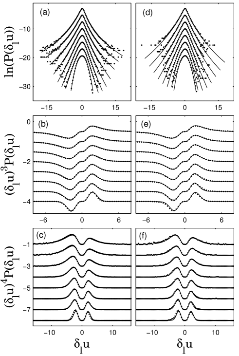
The PDFs of longitudinal velocity increments so-obtained from Eq. (8) are shown in Fig. 3 for several scales spanning the inertial and intermediate dissipative ranges, and compared to the experimental ones for both Air jet Fig. 3(a-c) and Modane 3(d-f). We see a continuous deformation across scales, from Gaussian at the correlation length scale () to exponential-like distributions in the inertial range and ultimately to stretched-exponential when dissipation starts acting. This PDF shape evolution is the signature of intermittency and is remarkably reproduced by our formalism when using the same quadratic parameter function and constant as in Figs. 1 and 2. This agreement is emphasized in Figs. (3)(b,d) and (3)(c,f) where respectively and are represented as a quantitative test of the relevance of our formalism to account for the dissymmetrical PDF tails.
5 Conclusion
To conclude, we have shown that the evolution across scales of the signed longitudinal velocity increments statistics, from the inertial far down the dissipative ranges, depends only on a universal parameter function and a universal constant that must be seen as a multifractal version of the Kolmogorov constant. In particular, neglecting the intermittency corrections, we provide an enhanced phenomenology of turbulence in deriving the value of the Skewness in the inertial range. We have further shown that choosing a quadratic form for (i.e. the hallmark of an underlying lognormal cascading process) provides a very good quantitative description of the longitudinal velocity increments PDFs measured in several flows, in different geometries and for different Reynolds numbers. This study proposes a new formalism, relying on the Edgeworth’s development, which opens the route to the modeling of velocity increment PDF. New experimental investigations of velocity gradients statistics would be welcomed as an additional and complementary test of our theoretical multifractal approach.
We wish to acknowledge P. Flandrin for fruitful discussions.
Appendix A Multifractal prediction of the Skewness of derivatives
In an infinite domain, or in a finite domain with periodic boundary conditions, a Taylor’s development of the second order structure function leads to
| (11) |
Inserting the development pointed by Eq. (11) into the Kármán-Howarth-Kolmogorov equation (Eq. (6)) leads to
| (12) |
This classical result can be found in Ref. [24]. One may wonder whether our description of the second order structure function (Eqs. (2) and (3)) is consistent with this development (Eq. (11)). In particular, the pre-supposed continuous and differentiable transition between the inertial and the dissipative range of scale inspired from the work of Batchelor [13] should give a leading term proportional to once inserted in Eq. (6). This property constrains seriously the possible form of the transition. The transition form used here benefits of such property. We get, with the help of a symbolic calculation software,
| (13) |
where is a negligible additive term, coming from the Taylor’s development of the normalization factor , and given by
| (14) |
| 208 | 0.35 | 0.17 |
| 380 | 0.38 | 0.17 |
| 2500 | 0.50 | 0.17 |
Eq. (13) can be seen as the multifractal prediction of the third order moment of the velocity derivatives, using the same transition interpolation form as in Eqs. (2) and (3). This is also a prediction for the second order moment of the second order derivative of velocity via Eq. (12). We gather in Table 1 the theoretical values for the Skewness and the Asymmetric factor , i.e. the limit when of our theoretical predictions for the Skewness and Asymmetric factor of velocity increments presented in Fig. 2. A specifically designed experiment aimed at measuring the fluctuations of longitudinal velocity increments for scale much smaller than the Kolmogorov length scale will provide a decisive test of the validity of these theoretical predictions.
References
- [1] U. Frisch, Turbulence (Cambridge University Press, Cambridge, 1995).
- [2] P. Kailasnath, K. R. Sreenivasan and G. Stolovitzky, Probability density of velocity increments in turbulent flows, Phys. Rev. Lett. 68, 2766 (1992).
- [3] L. Chevillard, B. Castaing and E. Lévêque, On the rapid increase of intermittency in the near-dissipation range of fully developed turbulence, Eur. Phys. J. B 45, 561 (2005).
- [4] G. Parisi and U. Frisch, in Turbulence and Predictability in Geophysical Fluid Dynamics, edited by M. Ghil, R. Benzi and G. Parisi (North-Holland, Amsterdam, 1985), p. 84.
- [5] G. Paladin and A. Vulpiani, Degrees of freedom of turbulence, Phys. Rev. A 35, 1971 (1987).
- [6] M. Nelkin, Multifractal scaling of velocity derivatives in turbulence, Phys. Rev. A 42, 7226 (1990).
- [7] U. Frisch and M. Vergassola, A prediction of the multifractal model : the intermediate dissipation range, Europhys. Lett. 14, 439 (1991).
- [8] C. Meneveau, On the transition between viscous and inertial-range scaling of turbulence structure functions, Phys. Rev. E 54, 3657 (1996).
- [9] B. Castaing, Y. Gagne and E. Hopfinger, Velocity probability density functions of high Reynolds number turbulence, Physica D 46, 177 (1990).
- [10] B. Castaing, Y. Gagne and M. Marchand, Log-similarity for turbulent flows ?, Physica D 68, 387 (1993).
- [11] D. Lohse, Crossover from high to low Reynolds number turbulence, Phys. Rev. Lett. 73, 3223 (1994).
- [12] Y. Gagne, B. Castaing, C. Baudet and Y. Malécot, Reynolds dependence of third-order velocity structure functions, Phys. Fluids 16, 482 (2004).
- [13] G. K. Batchelor, Pressure fluctuations in isotropic turbulence, Proc. Cambridge Philos. Soc. 47, 359 (1951).
- [14] L. Sirovich, L. Smith and V. Yakhot, Energy spectrum of homogeneous and isotropic turbulence in far dissipation range, Phys. Rev. Lett. 72, 344 (1994).
- [15] D. Lohse and A. Müller-Groeling, Bottleneck effects in turbulence: scaling phenomena in r versus p space, Phys. Rev. Lett. 74 1747 (1995).
-
[16]
L. Chevillard, PhD thesis
(2004). Available online at
http://tel.ccsd.cnrs.fr - [17] L. Chevillard, S. G. Roux, E. Lévêque, N. Mordant, J.-F. Pinton, and A. Arneodo, Lagrangian velocity statistics in turbulent flows: effects of dissipation, Phys. Rev. Lett. 91, 214502 (2003).
- [18] L. Biferale, G. Boffetta, A. Celani, B. J. Devenish, A. Lanotte and F. Toschi, Multifractal statistics of Lagrangian velocity and acceleration in turbulence, Phys. Rev. Lett. 93, 064502 (2004).
- [19] J. Delour, J.-F. Muzy, and A. Arneodo, Intermittency of 1d velocity spatial profiles in turbulence : a magnitude cumulant analysis, Eur. Phys. J. B 23, 243 (2001).
- [20] O. Chanal, B. Chabaud, B. Castaing and B. Hébral, Intermittency in a turbulent low temperature gaseous helium jet, Eur. Phys. J. B 17, 309 (2000).
- [21] G. Ruiz-Chavarria, C. Baudet, and S. Ciliberto, Hierarchy of the energy dissipation moments in fully developed turbulence, Phys. Rev. Lett. 74, 1986 (1995).
- [22] H. Kahalerras, Y. Malécot, Y. Gagne and B. Castaing, Intermittency and Reynolds number, Phys. Fluids 10, 910 (1998).
- [23] A. Arneodo, S. Manneville and J.-F. Muzy, Towards log-normal statistics in high Reynolds number turbulence, Eur. Phys. J. B 1, 129 (1998).
- [24] A. S. Monin and A. M. Yaglom, Statistical Fluid Mechanics (MIT Press, Cambridge, 1971).
- [25] J. Qian, Closure approach to high-order structure functions of turbulence, Phys. Rev. Lett. 84, 646 (2000).
- [26] E. Lindborg, Correction to the four-fifths law due to variations of the dissipation, Phys. Fluids 11, 510 (1999).
- [27] T. Lundgren, Kolmogorov two-thirds law by matched asymptotic expansion, Phys. Fluids 14, 638 (2002).
- [28] C. W. Van Atta and R. Antonia, Reynolds number dependence of skewness and flatness factors of turbulent velocity derivatives, Phys. Fluids 23, 252 (1980).
- [29] P. Tabeling, G. Zocchi, F. Belin, J. Maurer and H. Willaime, Probability density functions, skewness, and flatness in large Reynolds number turbulence, Phys. Rev. E 53, 1613 (1996).
- [30] K. R. Sreenivasan and R. A. Antonia, The phenomenology of small-scale turbulence, Annu. Rev. Fluid Mech. 29, 435 (1997).
- [31] H.S. Kang, S. Chester and C. Meneveau, Decaying turbulence in an active-grid-generated flow and comparisons with large-eddy simulation, J. Fluid Mech. 480, 129 (2003).
- [32] P. McCullagh, Tensor Methods in Statistics, Chapman and Hall, London (1987).