Scaling and Universality in the Counterion-Condensation Transition
at Charged Cylinders

Abstract

Counterions at charged rod-like polymers exhibit a condensation transition at a critical temperature (or equivalently, at a critical linear charge density for polymers), which dramatically influences various static and dynamic properties of charged polymers. We address the critical and universal aspects of this transition for counterions at a single charged cylinder in both two and three spatial dimensions using numerical and analytical methods. By introducing a novel Monte-Carlo sampling method in logarithmic radial scale, we are able to numerically simulate the critical limit of infinite system size (corresponding to infinite-dilution limit) within tractable equilibration times. The critical exponents are determined for the inverse moments of the counterionic density profile (which play the role of the order parameters and represent the inverse localization length of counterions) both within mean-field theory and within Monte-Carlo simulations. In three dimensions, we demonstrate that correlation effects (neglected within mean-field theory) lead to an excessive accumulation of counterions near the charged cylinder below the critical temperature (condensation phase), while surprisingly, the critical region exhibits universal critical exponents in accord with the mean-field theory. Also in contrast with the typical trend in bulk critical phenomena, where fluctuations are strongly enhanced in lower dimensions, we demonstrate, using both numerical and analytical approaches, that the mean-field theory becomes exact for the 2D counterion-cylinder system at all temperatures (Manning parameters), when number of counterions tends to infinity. For finite particle number, however, the 2D problem displays a series of peculiar singular points (with diverging heat capacity), which reflect successive de-localization events of individual counterions from the central cylinder. In both 2D and 3D, the heat capacity shows a universal jump at the critical point, and the energy develops a pronounced peak. The asymptotic behavior of the energy peak location is used to locate the critical point, which is also found to be universal and in accordance with the mean-field prediction.

I Introduction

Electrostatics of charged polymers is often dominated by small oppositely charged ions (counterions), which maintain the global electroneutrality of charged solutions. Many charged polymers, such as tubulin, actin and DNA are stiff and may be represented by straight cylinders (on length scales smaller than the persistence length). Neglecting many-ion effects, a single counterion is attracted by an electrostatic potential that grows logarithmically with the radial distance from the central cylinder axis. But since the counterion confinement entropy also shows a logarithmic size dependence, it was suggested early by Onsager Manning69 that a counterion delocalization transition occurs at a critical cylinder charge or equivalently, at a critical temperature. Onsager’s argument, which is strictly valid for a single particle, was soon corroborated by mean-field studies Manning69 ; Oosawa ; Oosawa_Imai ; Manning77 ; Manning_Dyn ; Manning_rev78 ; Manning_rev96a ; Manning_rev96b ; Macgillivray ; Ramanathan ; Ramanathan_Wood82a ; Ramanathan_Wood82b ; Zimm , which demonstrate that a charged cylinder can indeed bind or condense a finite fraction of counterions below a critical temperature (and even in the limit of infinite system size with no confining boundaries), while above the critical temperature, all counterions de-condense and diffuse to infinity.

This counterion-condensation transition (CCT) dramatically affects a whole number of static and dynamic quantities as observed in recent experiments on charged polymers Oosawa ; Manning_rev78 ; Manning_rev96a ; Ikegami ; Zana ; Zema81 ; Klein84 ; Ander84 ; Penaf92 ; Hoagland03 : upon condensation, the bare polymer charge is screened leading, for instance, to a significant reduction in electrophoretic mobility Klein84 ; Hoagland03 and conductivity of polymers Penaf92 ; it also triggers striking static properties such as counterion-induced attraction between like-charged polymers, which gives rise to compact phases of F-actin Tang and DNA Bloom . Since its discovery, the CCT has been at the focus of numerical Winkler98 ; Deserno00 ; Liu_Muthu02 ; Liao03 and analytical Fixman79 ; Stigter ; de-la-Cruz95 ; Tracy97 ; Levin97 ; Levin98 ; Schiess98 ; Nyquist99 ; Ray_Mann99 ; Qian00 ; Manning01 ; Rubinstein01 ; Rudi01 ; Henle04 ; Muthu04 ; Borukhov04 ; Shaugh ; Naji_CC studies. Under particular dispute has been the connection between CCT and the celebrated Kosterlitz-Thouless transition of logarithmically interacting particles in two dimensions Levin97 ; Kholod95_KT ; Levin98_KT ; Suzuki04 .

The CCT at charged cylinders is regulated by a dimensionless control parameter, $\xi=q\ell_{\mathrm{B}}\tau$, known as the Manning parameter Manning69 , which depends on the linear charge density of the cylinder, $-\tau e$, charge valency of counterions, $+q$, and the Bjerrum length $\ell_{\mathrm{B}}=e^{2}/(4\pi\varepsilon\varepsilon_{0}k_{\mathrm{B}}T)$ accommodating the ambient temperature $T$ and the medium dielectric constant $\varepsilon$. The Manning parameter plays the role of the inverse rescaled temperature and can be varied experimentally by changing the linear charge density (using synthetic chains or various $p$H) Zema81 ; Ander84 ; Penaf92 ; Hoagland03 or by varying the dielectric media (mixing different solvents) Klein84 ; Hoagland03 . According to mean-field theory Manning69 ; Oosawa ; Macgillivray ; Ramanathan ; Ramanathan_Wood82a ; Ramanathan_Wood82b ; Zimm , condensation occurs above the critical value $\xi_{c}=1$. In experiments, the critical Manning parameter appears to be about unity, but large deviations have also been reported Penaf92 ; Hoagland03 ; Cleland91 , and the precise location of the critical point is still debated Hoagland03 .

On the other hand, it is known that the critical temperature may in general be influenced by correlations and fluctuations, which are not captured within the mean-field theory critical . These effects typically cause deviations from mean-field predictions in both non-universal and universal quantities below the upper critical dimension. Surprisingly, the mean-field prediction for the CCT threshold, $\xi_{c}$, has not been questioned in literature and apparently assumed to be exact. Likewise, the existence of universal scaling relations and critical (scaling) exponents associated with the CCT has not been addressed, neither on the mean-field level nor in the presence of correlations.

Our chief goal in this paper is to address the following issues: i) what is the exact threshold of the CCT, $\xi_{c}$, and ii) what are the critical exponents associated with this transition both in three and two spatial dimensions. We shall also address the type of singularities that emerge in thermodynamic quantities as the CCT criticality sets in. To establish a systematic investigation of the correlation effects, we employ Monte-Carlo simulations for counterions at a single charged cylinder using a novel sampling method (centrifugal sampling), which is realized by mapping the radial coordinate to a logarithmic scale. This enables us to investigate the critical limit of infinite system size (that is when the outer boundaries confining counterions tend to infinity) within tractable equilibration times in the simulations. The importance of taking very large system sizes becomes evident by noting that lateral finite-size effects, which mask the critical unbinding behavior of counterions, depend on the logarithm of system size in the cylindrical geometry Manning69 ; Manning77 ; Macgillivray ; Ramanathan ; Ramanathan_Wood82a ; Ramanathan_Wood82b ; Zimm ; Deserno00 ; Levin97 ; Levin98 ; Qian00 ; Rubinstein01 ; Shaugh ; Alfrey51 ; Fuoss51 , causing a quite weak convergence to the critical infinite-size limit.

Our simulations provide the first numerical results for the asymptotic critical behavior of CCT and systematically incorporate correlation effects (a brief report of some of our results has been presented previously Naji_CC ). The relevance of electrostatic correlations is in general identified by a dimensionless coupling parameter, $\Xi=2\pi q^{3}\ell_{\mathrm{B}}^{2}\sigma_{\mathrm{s}}$ with $\sigma_{\mathrm{s}}=\tau/(2\pi R)$ being the surface charge density and $R$ the radius of the cylinder. The mean-field theory represents the limit $\Xi\rightarrow 0$ Netz ; Andre , while in the converse limit of strong coupling, $\Xi\gg 1$, correlations become significant and typically lead to drastic changes Netz ; Andre ; Low_T ; Naji04 . In order to investigate scaling properties of the CCT in various regimes of the coupling parameter, we focus on the inverse moments of the counterionic density profile, which play the role of the “order parameters” for this transition and represent the mean inverse localization length of counterions. Using a combined finite-size-scaling analysis with respect to both lateral size of the system and the number of counterions, we show that the order parameters adopt scale-invariant forms in the vicinity of the critical point. The critical exponents associated with the reduced temperature and the size parameters are determined both within the simulations and also analytically within two limiting theories of mean field and strong coupling. As a main result, we find that the critical exponents of the CCT are universal (that is independent of the coupling parameter varied over several decades $0.1<\Xi<10^{5}$) and appear to be in close agreement with the mean-field prediction. Surprisingly, we find that the critical Manning parameter is also universal and given by the mean-field value $\xi_{c}=1$. The transition threshold, $\xi_{c}$, is determined with high accuracy from the asymptotic behavior of the location of a singular peak that emerges in average internal energy of the system. The excess heat capacity is found to vanish at small Manning parameters (de-condensation phase) and exhibits a universal jump at the transition point indicating that the CCT may be regarded as a second-order phase transition as also suggested in a previous mean-field study Rubinstein01 .

As will be shown, the validity of mean-field predictions in 3D breaks down as the Manning parameter increases beyond the critical value (i.e. in the condensation phase), where inter-particle correlations become significant at large couplings. This leads to an enhanced accumulation of counterions near the cylinder surface and a crossover to the strong-coupling theory predictions Netz ; Andre ; Naji_PhysicaA .

In order to bring out possible role of fluctuations, we also study the CCT in a 2D counterion-cylinder system (equivalent to a 3D system composed of a central charged cylinder and parallel cylindrical “counterions” with logarithmic Coulomb interactions, as may be applicable to an experimental system of oriented cationic and anionic polymers, e.g., DNA with polylysine Jason ). For finite number of counterions, a peculiar series of singular points emerge that reflect delocalization events of individual counterions as the Manning parameter varies. For increasing particle number, the singular points tend to merge and eventually in the thermodynamic limit, the 2D results tend to universal values determined by the mean-field theory. Therefore, in contrast to the typical trend in critical phenomena, the CCT in 2D is found to be in exact agreement with the mean-field theory for the whole range of Manning parameters (or temperatures) when the number of counterions tends to infinity. As will be shown, the simulation results in 2D can be reproduced using an approximate analytical approach. A more systematic method has been developed recently Burak_unpub supporting the present analytical results.

The organization of the paper is as follows: in Sections II-VI, we focus on the counterion-cylinder system in three spatial dimensions. Our model is introduced in Section II, where we shall also outline the general method proposed for the investigation of the CCT. In Section III, we derive the scaling relations for order parameters and determine the asymptotic behavior of thermodynamic quantities within the mean-field theory (which is valid in all dimensions). In Section IV, analytical results are obtained within the strong-coupling theory. The numerical analysis of the CCT for various coupling strength will be presented in Sections VI and VII in three and two dimensions, respectively.

II Counterion-condensation transition (CCT) in three dimensions

II.1 Cell model for charged rod-like polymers

We consider a primitive cell model Alfrey51 ; Fuoss51 ; Lifson54 , which consists of a single charged cylinder of radius $R$ and point-like neutralizing counterions of charge valency $+q$ that are confined laterally in an outer (co-axial) cylindrical box of radius $D$–see Figure 1. The cylinder has infinite length, $L$, and a uniform (surface) charge distribution, $-\sigma({\mathbf{x}})e$, where $\sigma({\mathbf{x}})=\sigma_{\mathrm{s}}\delta(r-R)$. (Note that $q$ and $\sigma_{\mathrm{s}}$ are given in units of the elementary charge, $e$, and are positive by definition.) The cylinder is assumed to be rigid and impenetrable to counterions and the dielectric medium is represented by a uniform dielectric constant, $\varepsilon$. In the three dimensions, electric charges interact via bare Coulombic interaction

$$v_{\mathrm{3D}}({\mathbf{x}})=1/|{\mathbf{x}}|.$$ (1)

The electroneutrality condition holds globally inside the cell and entails the relation

$$qN=\tau L,$$ (2)

where $N$ is the number of counterions per cell and $\tau=2\pi R\sigma_{\mathrm{s}}$ represents the linear charge density of the cylinder. The system is described by the Hamiltonian

$$\frac{{\mathcal{H}}_{N}}{k_{\mathrm{B}}T} = q^{2}\ell_{\mathrm{B}}\sum_{\langle ij\rangle}v_{\mathrm{3D}}({\mathbf{x}}_{i}-{\mathbf{x}}_{j})$$ (3)

$$- q\ell_{\mathrm{B}}\sum_{i=1}^{N}\int\,v_{\mathrm{3D}}({\mathbf{x}}-{\mathbf{x}}_{i})\,\sigma({\mathbf{x}})\,{\mathrm{d}}{\mathbf{x}}$$

$$+ \frac{\ell_{\mathrm{B}}}{2}\int\,\sigma({\mathbf{x}})\,v_{\mathrm{3D}}({\mathbf{x}}-{\mathbf{x}}^{\prime})\,\sigma({\mathbf{x}}^{\prime})\,{\mathrm{d}}{\mathbf{x}}\,{\mathrm{d}}{\mathbf{x}}^{\prime},$$

which comprises mutual repulsions between counterions located at $\{{\mathbf{x}}_{i}\}$ (first term), the counterion-cylinder attraction (second term) and the self-energy of the cylinder (last term). It can be written as

$$\frac{{\mathcal{H}}_{N}}{k_{\mathrm{B}}T}=q^{2}\ell_{\mathrm{B}}\sum_{\langle ij\rangle}v_{\mathrm{3D}}({\mathbf{x}}_{i}-{\mathbf{x}}_{j})+2\xi\sum_{i=1}^{N}\ln\left(\frac{r_{i}}{R}\right)+C_{0},$$ (4)

where $\xi$ is the Manning parameter of the system Manning69 ; Manning77 ,

$$\xi=q\ell_{\mathrm{B}}\tau$$ (5)

with $\ell_{\mathrm{B}}=e^{2}/(4\pi\varepsilon\varepsilon_{0}k_{\mathrm{B}}T)$ being the Bjerrum length (in water and at room temperature $\ell_{\mathrm{B}}\simeq 7$Å), and $r_{i}=(x_{i}^{2}+y_{i}^{2})^{1/2}$ being the radial coordinate of the $i$-th counterion from the cylinder axis, which coincides with $z$-axis. The additive term $C_{0}$ in Eq. (4) is related to the cylinder self-energy, which will be important in obtaining a convergent energy expression for the system in the simulations (Section V.2 and Appendix D).

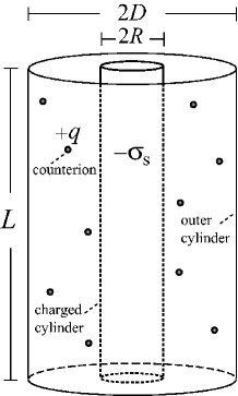
Figure 1: The three-dimensional model consists of a charged cylinder of infinite length, $H$, and its neutralizing counterions confined in an outer cylindrical box (see the text for parameters).

II.2 Dimensionless description

The parameter space of the system may be spanned by a minimal set of independent dimensionless parameters obtained from the ratios between characteristic length scales. These length scales are the rescaled Bjerrum length, $q^{2}\ell_{\mathrm{B}}$, the Gouy-Chapman length

$$\mu=\frac{1}{2\pi q\ell_{\mathrm{B}}\sigma_{\mathrm{s}}},$$ (6)

and the radius of the charged cylinder, $R$, and that of the outer boundary, $D$. The rescaled cylinder radius

$$\tilde{R}=\frac{R}{\mu}=\xi$$ (7)

equals the Manning parameter, $\xi$. The ratio between the rescaled Bjerrum length and the Gouy-Chapman length, $\mu$, gives the so-called electrostatic coupling parameter Netz ,

$$\Xi=\frac{q^{2}\ell_{\mathrm{B}}}{\mu}=2\pi q^{3}\ell_{\mathrm{B}}^{2}\sigma_{\mathrm{s}},$$ (8)

which can identify the importance of electrostatic correlations in a charged system Netz ; Andre ; Naji04 ; Naji_PhysicaA , and the ratio between $D$ and $R$, which enters only through the lateral extension parameter

$$\Delta\equiv\ln\left(\frac{D}{R}\right)$$ (9)

characterizing lateral finite-size effects. The relevant infinite-system-size limit is obtained for $\Delta\rightarrow\infty$ Zimm ; Alfrey51 ; Fuoss51 .

We shall use the dimensionless form of the Hamiltonian obtained by rescaling the spatial coordinates as ${\tilde{\mathbf{x}}}={\mathbf{x}}/\mu$ Netz , that is

$$\frac{{\mathcal{H}}_{N}}{k_{\mathrm{B}}T}=\Xi\sum_{\langle ij\rangle}v_{\mathrm{3D}}({\tilde{\mathbf{x}}}_{i}-{\tilde{\mathbf{x}}}_{j})+2\xi\sum_{i=1}^{N}\ln\left(\frac{{\tilde{r}}_{i}}{\tilde{R}}\right)+C_{0}.$$ (10)

The electroneutrality condition (2) in rescaled units reads

$$2\pi\xi{\tilde{L}}=2\pi\Xi N,$$ (11)

where the left hand side is simply the rescaled area of the cylinder covered by the electric charge. The thermodynamic limit is obtained for $N\rightarrow\infty$ and $L\rightarrow\infty$, but keeping $N/L=\tau/q$ (or equivalently, $N/\tilde{L}=\xi/\Xi$) fixed.

II.3 CCT as a generic binding-unbinding process

The statistical physical properties of the system may be investigated using the canonical partition function,

$${\mathcal{Z}}_{N}=\frac{\mu^{3N}}{N!}\int_{\tilde{V}}\left[\prod_{i=1}^{N}{\mathrm{d}}{\tilde{z}}_{i}\,{\mathrm{d}}\phi_{i}\,{\mathrm{d}}{\tilde{r}}_{i}\,{\tilde{r}}_{i}\right]\exp\bigg{\{}-\frac{{\mathcal{H}}_{N}}{k_{\mathrm{B}}T}\bigg{\}}$$ (12)

represented in cylindrical coordinates ${\tilde{\mathbf{x}}}_{i}=({\tilde{r}}_{i},\phi_{i},{\tilde{z}}_{i})$, with the spatial integral running over the volume, $\tilde{V}$, of the space accessible for counterions, i.e. ${\tilde{R}}\leq{\tilde{r}}\leq{\tilde{D}}$.

Naively, one may conjecture that the partition function (12) diverges in a certain range of Manning parameters, when the upper boundary of the radial integrals, ${\tilde{D}}$, tends to infinity, as may be indicated by the logarithmic form of the counterion-cylinder interaction, which gives rise to algebraic prefactors of the form ${\tilde{r}}_{i}^{1-2\xi}$ in the integrand. The possible emergence of a divergency in a charged cylindrical system was first pointed out by Onsager and the connection with the counterion-condensation transition was discussed by Manning Manning69 .

Here we demonstrate this peculiar point using a transformation of coordinates, which provides the basis for our numerical simulations considered later in Sections V and VI. The radial coordinate is transformed as

$$y=\ln\left(\frac{\tilde{r}}{\tilde{R}}\right),$$ (13)

upon which the partition function in (12) transforms as

$${\mathcal{Z}}_{N}=\frac{\mu^{3N}{\tilde{R}}^{2N}}{N!}\int_{\tilde{V}}\left[\prod_{i=1}^{N}{\mathrm{d}}{\tilde{z}}_{i}\,{\mathrm{d}}\phi_{i}\,{\mathrm{d}}y_{i}\right]\exp\bigg{\{}-\frac{{\mathcal{H}}_{N}^{\ast}}{k_{\mathrm{B}}T}\bigg{\}},$$ (14)

where the volume integral runs over the region $0<y<\Delta=\ln(D/R)$, and

$$\frac{{\mathcal{H}}_{N}^{\ast}}{k_{\mathrm{B}}T}=\sum_{i=1}^{N}W(y_{i})+\Xi\sum_{\langle ij\rangle}v_{\mathrm{3D}}({\tilde{\mathbf{x}}}_{i}-{\tilde{\mathbf{x}}}_{j})+C_{0}$$ (15)

is the transformed Hamiltonian of the system with

$$W(y)=2(\xi-1)y.$$ (16)

As seen, the original partition function is now mapped to the partition function of a system of interacting (repelling) particles in a linear potential well, $W(y)$. This virtual potential includes the contributions associated with the cylindrical boundary, namely, the bare counterion-cylinder attraction (i.e. $2\xi y$) and an entropic (repulsive) term from the measure of the radial integral (i.e. $2y$), which may be regarded as an induced centrifugal component.

For small Manning parameter, $\xi<1$, the potential well, $W(y)$, becomes purely repulsive suggesting that counterions unbind (or “de-condense”) from the central cylinder departing to infinitely large distances as the outer confining boundary tends to infinity, $\Delta=\ln(D/R)\rightarrow\infty$. In contrast for $\xi>1$, the potential well exerts an attractive force upon counterions, which might lead to partial binding (or “condensation”) of counterions even in the absence of confining walls. The new representation of ${\mathcal{Z}}_{N}$ in Eq. (14), therefore, reflects the interplay between energetic and entropic factors on a microscopic level.

Note that the rigorous analytical derivation of the aforementioned properties for counterions based on the full partition function is still an open problem, and only approximate limiting cases have been examined analytically (Section II.5).

II.4 Onsager instability

As a simple illustrative case, let us consider a “hypothetical” system, in which mutual counterionic repulsions are switched off. The partition function (12) thus factorizes as ${\mathcal{Z}}_{N}\sim{\mathcal{Z}}_{1}^{N}$, where

$${\mathcal{Z}}_{1}=\int_{0}^{\Delta}{\mathrm{d}}y\,e^{(2-2\xi)y}=\frac{e^{(2-2\xi)\Delta}-1}{2-2\xi}$$ (17)

is the single-particle partition function. It diverges for $\xi<1$, when the lateral extension parameter, $\Delta$, tends to infinity, which implies complete de-condensation of counterions, i.e. the probability, $P(r)\sim\exp(-2\xi\ln r)/{\mathcal{Z}}_{1}$, of finding counterions at any finite distance, $r$, from the cylinder tends to zero (equivalent to a vanishing density profile, $\rho(r)=NP(r)$). But ${\mathcal{Z}}_{1}$ and the counterionic density profile remain finite for $\xi>1$, indicating that the Manning parameter $\xi_{c}=1$ is the onset of the CCT on the one-particle level, which we term here as the Onsager instability (in the spirit of Onsager’s original argument Manning69 ). Onsager instability captures the basic features of the CCT. It exhibits the weak logarithmic convergence (via $\Delta=\ln D/R$) to the critical limit as the volume per polymer ($\sim D^{2}$) goes to infinity Note_Ons , and as shown in Appendix A, displays algebraic singularities in energy and heat capacity (at $\xi_{c}=1$) that may be identified by a set of scaling exponents. Such scaling relations are crucial in our analysis of the CCT in the following sections.

We emphasize here that the results obtained within Onsager instability are by no means conclusive as soon as inter-counterionic interactions are switched on, which, as will be shown, lead to qualitative differences. In particular, it turns out that a diverging partition function is not necessarily an indication of the onset of the CCT as asserted by the single-particle argument Manning69 .

II.5 Beyond the Onsager instability: many-body effects and electrostatic correlations

Many-body terms involved in the full partition function (12) render the systematic analysis of the CCT quite difficult. The analytical results are available in the asymptotic limits of i) vanishingly small coupling parameter $\Xi\rightarrow 0$, which leads to the mean-field or Poisson-Boltzmann (PB) theory, and ii) for infinitely large coupling parameter $\Xi\rightarrow\infty$, which leads to the strong-coupling (SC) theory Netz . In the mean-field approximation (case i), statistical correlations among counterions are systematically neglected. In the opposite limit of strong coupling (case ii), the leading contribution to the partition function takes a very simple form comprising only the one-particle (counterion-cylinder) contributions, which is associated with strong electrostatic correlations (pronounced correlation hole) between counterions at the surface Netz ; Andre ; Naji04 ; Naji_PhysicaA ; Burak04 . We study the mean-field predictions for the CCT in Section III. The SC description ($\Xi\rightarrow\infty$) resembles the Onsager instability and will be discussed in Section IV and Appendix A. The perturbative improvement of these two limiting theories in a system of finite coupling parameter, $\Xi$, is formally possible by computing higher-order correction terms as previously performed for planar charged walls Netz ; Andre , but will not be considered here.

Interestingly, in both limits, the onset of the CCT is obtained as $\xi_{c}=1$, which is due to the simplified form of the counterionic correlations. An important question is whether the critical value, $\xi_{c}$, varies with the coupling parameter. Such a behavior may be expected since the Manning parameter represents the rescaled inverse temperature of the system (i.e. $\xi=T_{\ast}/T$ with $T_{\ast}\equiv q\tau e^{2}/(4\pi\varepsilon\varepsilon_{0}k_{\mathrm{B}})$), which, as known from bulk critical phenomena critical , can be shifted from its mean-field value due to inter-particle correlations for large couplings. Also it is interesting to examine whether the CCT exhibits scale-invariant properties near $\xi_{c}$ and if it can be classified in terms of a universal class of critical exponents. Such scaling relations are known to represent relevant statistical characteristics of systems close to continuous phase transitions critical .

To address these issues, one has to define quantities which can serve as order parameters of the CCT. In the following section, we shall introduce such quantities and, by considering the mean-field theory, show that the order parameters indeed exhibit scaling behavior near the CCT critical point. We return to the influence of electrostatic correlations on the critical Manning parameter and scaling exponents of the CCT in the subsequent sections.

III Mean-field theory for the counterion-condensation transition

III.1 Non-linear Poisson-Boltzmann (PB) equation

The mean-field theory can be derived systematically using a saddle-point analysis in the limit $\Xi\rightarrow 0$ Netz . It is governed by the well-known Poisson-Boltzmann (PB) equation Alfrey51 ; Fuoss51 , which, in rescaled units, reads (Appendix B)

$$\nabla^{2}_{{\tilde{\mathbf{x}}}}\psi=2{\tilde{\sigma}}({\tilde{\mathbf{x}}})-{\tilde{\kappa}}^{2}\,{\tilde{\Omega}}({\tilde{\mathbf{x}}})\,e^{-\psi({\tilde{\mathbf{x}}})}$$ (18)

for the dimensionless potential field $\psi({\tilde{\mathbf{x}}})$. Here

$${\tilde{\sigma}}({\tilde{\mathbf{x}}})=\delta({\tilde{r}}-{\tilde{R}})$$ (19)

is the rescaled charge distribution of the cylinder and

$${\tilde{\Omega}}({\tilde{\mathbf{x}}})={\tilde{\Omega}}({\tilde{r}})=\left\{\begin{array}[]{ll}1&{\,\,\,\,\,\,\,\,{\tilde{R}}\leq{\tilde{r}}\leq{\tilde{D}},}\\ \\ 0&{\,\,\,\,\,\,\,\,{\mathrm{otherwise}}}\end{array}\right.$$ (20)

specifies the volume accessible to counterions. In the canonical ensemble, one has

$$\frac{{\tilde{\kappa}}^{2}}{2}=\frac{2\pi\xi{\tilde{L}}}{\int{\mathrm{d}}{\tilde{\mathbf{x}}}\,{\tilde{\Omega}}({\tilde{\mathbf{x}}})\,\exp(-\psi)}.$$ (21)

Assuming the cylindrical symmetry (for an infinitely long cylinder) and using Eq. (18) and the global electroneutrality condition (11), one obtains

$$\left({\tilde{r}}\frac{{\mathrm{d}}\psi}{{\mathrm{d}}{\tilde{r}}}\right)_{{\tilde{r}}={\tilde{R}}}=2\xi\,\,\,\,\,{\mathrm{and}}\,\,\,\,\,\left({\tilde{r}}\frac{{\mathrm{d}}\psi}{{\mathrm{d}}{\tilde{r}}}\right)_{{\tilde{r}}={\tilde{D}}}=0,$$ (22)

which are used to solve the PB equation (18) in the non-trivial region ${\tilde{R}}\leq{\tilde{r}}\leq{\tilde{D}}$ Alfrey51 ; Fuoss51 . Thereby, one obtains both the free energy (Section III.3.2) and the rescaled radial density profile of counterions around the charged cylinder

$${\tilde{\rho}}({\tilde{r}})=\frac{{\tilde{\kappa}}^{2}}{2}{\tilde{\Omega}}({\tilde{r}})\,e^{-\psi({\tilde{r}})}.$$ (23)

The rescaled density profile, ${\tilde{\rho}}({\tilde{r}})$, is related to the actual number density of counterions, $\rho(r)$, through ${\tilde{\rho}}({\tilde{r}})=\rho(r)/(2\pi\ell_{\mathrm{B}}\sigma_{\mathrm{s}}^{2})$ Netz (Appendix B).

As shown by Alfrey et al. Alfrey51 and Fuoss et al. Fuoss51 , the PB solution takes different functional forms depending on whether $\xi$ lies below or above the Alfrey-Fuoss threshold

$$\Lambda_{\mathrm{AF}}=\frac{\Delta}{1+\Delta},$$ (24)

that is

$$\psi_{\mathrm{PB}}({\tilde{r}})=\left\{\begin{array}[]{ll}\ln[\frac{{\tilde{\kappa}}^{2}{\tilde{r}}^{2}}{2\beta^{2}}\sinh^{2}(\beta\ln\frac{{\tilde{r}}}{{\tilde{R}}}+\coth^{-1}\frac{\xi-1}{\beta})]&{\xi\leq\Lambda_{\mathrm{AF}},}\\ \\ \ln[\frac{{\tilde{\kappa}}^{2}{\tilde{r}}^{2}}{2\beta^{2}}\sin^{2}(\beta\ln\frac{{\tilde{r}}}{{\tilde{R}}}+\cot^{-1}\frac{\xi-1}{\beta})]&{\xi\geq\Lambda_{\mathrm{AF}},}\end{array}\right.$$ (28)

where $\beta$ is given by the transcendental equations

$$\xi=\left\{\begin{array}[]{ll}\frac{1-\beta^{2}}{1-\beta\coth(-\beta\Delta)}&{\,\,\,\,\,\xi\leq\Lambda_{\mathrm{AF}},}\\ \\ \frac{1+\beta^{2}}{1-\beta\cot(-\beta\Delta)}&{\,\,\,\,\,\xi\geq\Lambda_{\mathrm{AF}}.}\end{array}\right.$$ (32)

The PB density profile of counterions, Eq. (23), is then obtained for ${\tilde{R}}\leq{\tilde{r}}\leq{\tilde{D}}$ as

$${\tilde{\rho}}_{\mathrm{PB}}({\tilde{r}})=\frac{\beta^{2}}{{\tilde{r}}^{2}}\times\left\{\begin{array}[]{ll}\sinh^{-2}(\beta\ln\frac{{\tilde{r}}}{{\tilde{R}}}+\coth^{-1}\frac{\xi-1}{\beta})&{\xi\leq\Lambda_{\mathrm{AF}},}\\ \\ \sin^{-2}(\beta\ln\frac{{\tilde{r}}}{{\tilde{R}}}+\cot^{-1}\frac{\xi-1}{\beta})&{\xi\geq\Lambda_{\mathrm{AF}},}\end{array}\right.$$ (36)

where we have arbitrarily chosen $\psi_{\mathrm{PB}}({\tilde{r}}={\tilde{R}})=0$ to fix the reference of the potential. This condition also fixes ${\tilde{\kappa}}$ in Eq. (28) as well as the radial density of counterions at contact with the cylinder using Eq. (23), i.e.

$$\frac{{\tilde{\kappa}}^{2}}{2}={\tilde{\rho}}_{\mathrm{PB}}({\tilde{R}})=\frac{1}{\xi^{2}}\times\left\{\begin{array}[]{ll}(\xi-1)^{2}-\beta^{2}&{\,\,\,\,\xi\leq\Lambda_{\mathrm{AF}},}\\ \\ (\xi-1)^{2}+\beta^{2}&{\,\,\,\,\xi\geq\Lambda_{\mathrm{AF}}.}\end{array}\right.$$ (40)

The density profiles given in Eq. (36) are in fact normalized to the total number of counterions, $N$, a condition imposed via Eq. (21). Using Eq. (23), the normalization condition in rescaled units reads (Appendix B)

$$\int_{\tilde{R}}^{\tilde{D}}{\mathrm{d}}{\tilde{r}}\,{\tilde{r}}\,{\tilde{\rho}}_{\mathrm{PB}}({\tilde{r}})=\xi.$$ (41)

III.2 Onset of the CCT within mean-field theory

The threshold of CCT within the mean-field PB theory was considered by several workers Macgillivray ; Ramanathan ; Ramanathan_Wood82a ; Ramanathan_Wood82b ; Zimm ; Alfrey51 ; Fuoss51 . It may be obtained from the asymptotic behavior of the density profile ($\Delta\rightarrow\infty$) as reviewed below.

First note that for $\Delta\gg 1$, the Alfrey-Fuoss threshold $\Lambda_{\mathrm{AF}}$, Eq. (24), tends to unity from below, i.e.

$$\Lambda_{\mathrm{AF}}=1-\frac{1}{\Delta}+{\mathcal{O}}(\Delta^{-2}).$$ (42)

Therefore, for Manning parameter $\xi<1$, one may use the first relation in Eq. (32) to obtain the limiting behavior of the integration constant $\beta$ as (Appendix C.1)

$$\beta=(1-\xi)+{\mathcal{O}}\bigg{(}e^{-2\Delta(1-\xi)}\bigg{)},$$ (43)

when $\Delta\rightarrow\infty$. Using this into Eq. (40), one finds that the density of counterions at contact, ${\tilde{\rho}}_{\mathrm{PB}}({\tilde{R}})$, asymptotically vanishes. Hence, the density profile (23) at any finite distance from the cylinder tends to zero for $\xi\leq 1$, i.e.

$${\tilde{\rho}}_{\mathrm{PB}}({\tilde{r}})\rightarrow 0,$$ (44)

representing the de-condensation regime in the limit $\Delta\rightarrow\infty$. For $\xi\geq 1$, on the other hand, one has $\beta\rightarrow 0$ for increasing $\Delta$ (Appendix C.1), and thus using Eq. (40),

$${\tilde{\rho}}_{\mathrm{PB}}({\tilde{R}})\rightarrow\frac{(\xi-1)^{2}}{\xi^{2}}.$$ (45)

Using the second relation in Eq. (36) and expanding for small $\beta$, the radial density profile follows as Ramanathan ; Netz_Joanny

$${\tilde{\rho}}_{\mathrm{PB}}({\tilde{r}})\rightarrow\frac{(\xi-1)^{2}}{\xi^{2}}\left[\frac{\tilde{r}}{\tilde{R}}\right]^{-2}\left[1+(\xi-1)\ln\frac{\tilde{r}}{\tilde{R}}\right]^{-2}$$ (46)

in the limit $\Delta\rightarrow\infty$ (see also Appendix C.4), which is finite and indicates condensation of counterions. This proves that the mean-field critical point is given by

$$\xi_{c}^{\mathrm{PB}}=1,$$ (47)

corresponding to the mean-field critical temperature

$$T_{c}^{\mathrm{PB}}=\frac{q\tau e^{2}}{4\pi\varepsilon\varepsilon_{0}k_{\mathrm{B}}}.$$ (48)

III.3 Critical scaling-invariance: Mean-field exponents

It is readily seen from Eqs. (45) and (46) that the asymptotic density of counterions admits a scale-invariant or homogeneous form with respect to the reduced Manning parameter,

$$\zeta=1-\frac{\xi_{c}^{\mathrm{PB}}}{\xi},$$ (49)

close to the critical value $\xi_{c}^{\mathrm{PB}}=1$. Note that the reduced Manning parameter equals the reduced temperature of the system, $t=1-(T/T^{\mathrm{PB}}_{c})$, when other quantities such as the dielectric constant, $\varepsilon$, and the linear charge density of the cylinder, $\tau$, are kept fixed. (Experimentally, however, the Manning parameter may be varied by changing $\varepsilon$ Klein84 ; Hoagland03 or $\tau$ Zema81 ; Ander84 ; Penaf92 ; Hoagland03 at constant temperature, in which case, $\zeta$ can be related to the reduced dielectric constant or the reduced linear charge density.)

In a finite confining volume (finite $\Delta$), such scaling forms with respect to $\zeta$ do not hold since the true CCT is suppressed. Yet as a general trend critical , we expect that for sufficiently large $\Delta$, the reminiscence of such scaling relations appears in the form of finite-size-scaling relations near the transition point. These relations would involve both $\zeta$ and the lateral extension parameter, $\Delta$, (as the only relevant parameters in the mean-field limit) in a scale-invariant fashion as will be shown below.

III.3.1 The CCT order parameters

As possible candidates for the CCT “order parameter”, we use the inverse moments of the counterionic density profile

$$S_{n}(\xi,{\tilde{D}})\equiv\bigg{\langle}\frac{1}{{\tilde{r}}^{n}}\bigg{\rangle}=\frac{\int_{\tilde{R}}^{\tilde{D}}\,{\tilde{r}}\,{\mathrm{d}}{\tilde{r}}\,\,{\tilde{r}}^{-n}\,{\tilde{\rho}}({\tilde{r}})}{\int_{\tilde{R}}^{\tilde{D}}\,{\tilde{r}}\,{\mathrm{d}}{\tilde{r}}\,{\tilde{\rho}}({\tilde{r}})}$$ (50)

where $n>0$ Note_Sn . Note that these quantities reflect mean inverse localization length of counterions. In the condensation phase (where counterions adopt a finite density profile), one has $S_{n}>0$, reflecting a finite localization length. But at the critical point and in the de-condensation phase (with vanishing counterionic density profile), one has $S_{n}=0$ in the limit of infinite system size $\Delta\rightarrow\infty$, which indicates a diverging counterion localization length.

In order to derive the mean-field finite-size-scaling relations for $S_{n}$ near $\xi_{c}^{\mathrm{PB}}=1$, we focus on the PB solution in the regime of Manning parameters $\xi\geq\Lambda_{\mathrm{AF}}$, since for any finite $\Delta$, we have $\Lambda_{\mathrm{AF}}\leq\xi_{c}^{\mathrm{PB}}=1$ from Eq. (42). Inserting the first relation in Eq. (36) into Eq. (50), we obtain

$$S_{n}^{\mathrm{PB}}=\frac{\beta^{2}}{\xi}\int_{\tilde{R}}^{\tilde{D}}{\mathrm{d}}{\tilde{r}}\,\,{\tilde{r}}^{-n-1}\sin^{-2}(\beta\ln\frac{{\tilde{r}}}{{\tilde{R}}}+\cot^{-1}\frac{\xi-1}{\beta}).$$ (51)

Changing the integration variable as $y=\ln({\tilde{r}}/{\tilde{R}})$, we get

$$S_{n}^{\mathrm{PB}}=\frac{\beta^{2}}{\xi^{n+1}}\int_{0}^{\Delta}{\mathrm{d}}y\,e^{-ny}\sin^{-2}(\beta y+\cot^{-1}\frac{\xi-1}{\beta}).$$ (52)

For $\Delta\gg 1$, the above relation may be approximated by a simple analytic expression as (Appendix C.3)

$$S_{n}^{\mathrm{PB}}(\zeta,\Delta)\simeq\frac{1}{n}\bigg{[}\zeta^{2}+\beta^{2}(\zeta,\Delta)\bigg{]}$$ (53)

for $\xi$ being sufficiently close to the critical value $\xi_{c}^{\mathrm{PB}}=1$.

Using the above result, we may distinguish two limiting cases, where different scaling relations are obtained, namely, i) when $\Delta\rightarrow\infty$ but $\zeta=1-\xi_{c}^{\mathrm{PB}}/\xi$ is finite and close to the critical value $\zeta^{\mathrm{PB}}=0$, and ii) when $\Delta$ is finite and large, but the system tends towards the critical point, $\zeta\rightarrow\zeta_{c}^{\mathrm{PB}}=0$.

In the first case, as stated before, we have $\beta\rightarrow 0$ for the above-threshold regime, $\zeta\geq 0$; thus using Eq. (53), we obtain

$$S_{n}^{\mathrm{PB}}(\zeta,\Delta\rightarrow\infty)\simeq\frac{\zeta^{2}}{n}.$$ (54)

On the other hand, $S_{n}^{\mathrm{PB}}$ vanishes for $\zeta\leq 0$ (Appendix C.3). Hence, the following scaling relation is obtained in the infinite-system-size limit $\Delta\rightarrow\infty$,

$$S_{n}^{\mathrm{PB}}(\zeta,\infty)\simeq\left\{\begin{array}[]{ll}\zeta^{\chi_{\mathrm{PB}}}/n&{\,\,\,\,0\leq\zeta\ll 1,}\\ \\ 0&{\,\,\,\,\zeta\leq 0,}\end{array}\right.$$ (55)

which introduces the mean-field critical exponent associated with the reduced Manning parameter, $\zeta$ (or the reduced temperature, $t$) as

$$\chi_{\mathrm{PB}}=2.$$ (56)

The mean-field counterion-condensation transition is therefore characterized by a diverging (localization) length scale $1/S_{1}^{\mathrm{PB}}\sim\zeta^{-2}$, as the critical point is approached from above. The scaling relation (55) may also be derived in a direct way by considering a strictly infinite system ($\Delta=\infty$) as shown in Appendix C.4.

In the limiting case (ii) with $\zeta\rightarrow\zeta_{c}^{\mathrm{PB}}=0$, we have from Eq. (32) that $\beta\simeq\pi/(2\Delta)$ when $\Delta$ is finite but large, $\Delta\gg 1$ (Appendix C.1). Therefore, using Eq. (53) we obtain

$$S_{n}^{\mathrm{PB}}(0,\Delta)\simeq\frac{\pi^{2}}{4n\Delta^{2}},$$ (57)

which introduces a new scaling relation

$$S_{n}^{\mathrm{PB}}(0,\Delta)\sim\Delta^{-\gamma_{\mathrm{PB}}}$$ (58)

with the mean-field critical exponent

$$\gamma_{\mathrm{PB}}=2$$ (59)

associated with the lateral extension parameter, $\Delta$. This relation shows that the approach to the true CCT limit (when $S_{n}^{\mathrm{PB}}$ vanishes at the critical point) is logarithmically weak as the box size, $D$, increases to infinity, i.e. $S_{n}^{\mathrm{PB}}(\zeta=0)\sim 1/(\ln D/R)^{2}$.

The scaling relations (54) and (57) indicate that $S_{n}^{\mathrm{PB}}$ takes a general scale-invariant form with respect to $\zeta$ and $\Delta$ as

$$S_{n}^{\mathrm{PB}}\simeq\Delta^{-\gamma_{\mathrm{PB}}}{\mathcal{D}}_{n}(\zeta\Delta^{\gamma_{\mathrm{PB}}/\chi_{\mathrm{PB}}})$$ (60)

for sufficiently large $\Delta$ and in the vicinity of the mean-field critical point. The scaling function, ${\mathcal{D}}_{n}(u)$, has the following asymptotic behavior

$${\mathcal{D}}_{n}(u)\sim\left\{\begin{array}[]{ll}{\mathrm{const.}}&{\,\,\,\,u\rightarrow 0,}\\ \\ u^{\chi_{\mathrm{PB}}}/n&{\,\,\,\,u\rightarrow+\infty.}\end{array}\right.$$ (61)

In general, the scale-invariant relations such as Eq. (60) may be obtained within the PB frame-work using the fact that the integration constant $\beta(\zeta,\Delta)$ takes a scale-invariant form as

$$\beta\simeq\Delta^{-1}{\mathcal{B}}(\zeta\Delta).$$ (62)

Here ${\mathcal{B}}(u)$ is a scaling function which behaves asymptotically as (Appendix C)

$${\mathcal{B}}(u)\sim\left\{\begin{array}[]{ll}{\mathrm{const.}}&{\,\,\,\,u\rightarrow 0,}\\ \\ \sqrt{u}&{\,\,\,\,u\rightarrow+\infty.}\end{array}\right.$$ (63)

Combining Eqs. (53) and (62), the scaling function ${\mathcal{D}}_{n}(u)$ is obtained in terms of ${\mathcal{B}}(u)$ as

$${\mathcal{D}}_{n}(u)\simeq\frac{1}{n}\left[u^{2}+{\mathcal{B}}^{2}(u)\right],$$ (64)

which reproduces Eq. (61) when combined with Eq. (63).

The mean-field critical exponents $\chi_{\mathrm{PB}}$ and $\gamma_{\mathrm{PB}}$ appear to be independent of the order of the density moments, $n$. They may be used to characterize the mean-field universality class of the CCT in all dimensions, since the PB results are independent of the space dimensionality.

III.3.2 Mean-field energy and heat capacity

As shown in a previous work Naji03 , the mean-field canonical free energy of the counterion-cylinder system may be obtained using a saddle-point analysis from the field-theoretic representation of the partition function when $\Xi\rightarrow 0$ Netz . The rescaled PB free energy defined as ${\tilde{\mathcal{F}}}^{\mathrm{PB}}\equiv{\mathcal{F}}^{\mathrm{PB}}_{N}/(Nk_{\mathrm{B}}T)$, is given by (up to the trivial kinetic energy part)

$${\tilde{\mathcal{F}}}^{\mathrm{PB}}= - \frac{1}{\xi}\int{\tilde{r}}\,{\mathrm{d}}{\tilde{r}}\,\bigg{[}\frac{1}{4}\bigg{(}\frac{{\mathrm{d}}\psi_{\mathrm{PB}}}{{\mathrm{d}}\tilde{r}}\bigg{)}^{2}+\delta({\tilde{r}}-{\tilde{R}})\psi_{\mathrm{PB}}({\tilde{r}})\bigg{]}$$ (65)

$$- \ln\bigg{[}\frac{1}{\xi}\int_{\tilde{R}}^{\tilde{D}}\,{\tilde{r}}\,{\mathrm{d}}{\tilde{r}}\,e^{-\psi_{\mathrm{PB}}({\tilde{r}})}\bigg{]}-\ln\bigg{(}\frac{2V_{\mathrm{cyl}}}{N\xi}\bigg{)},\,\,\,$$

where $V_{\mathrm{cyl}}=\pi R^{2}L$ is the actual volume of the cylinder. In the thermodynamic limit $N\rightarrow\infty$, the ratio $V_{\mathrm{cyl}}/N$ is a constant and will be dropped in what follows.

Inserting the PB potential field, Eq. (28), into the free energy expression (65), we find that for $\xi>\Lambda_{\mathrm{AF}}$

$${\tilde{\mathcal{F}}}^{\mathrm{PB}}= - \frac{1}{\xi}\bigg{[}(1-\beta^{2})\Delta+\ln\left(\frac{(\xi-1)^{2}+\beta^{2}}{1+\beta^{2}}\right)+\xi\bigg{]}$$ (66)

$$+ \ln[(\xi-1)^{2}+\beta^{2}]-\ln(2\xi).$$

While for $\xi<\Lambda_{\mathrm{AF}}$, we have

$${\tilde{\mathcal{F}}}^{\mathrm{PB}}= - \frac{1}{\xi}\bigg{[}(1+\beta^{2})\Delta+\ln\left(\frac{(\xi-1)^{2}-\beta^{2}}{1-\beta^{2}}\right)+\xi\bigg{]}$$ (67)

$$+ \ln[(\xi-1)^{2}-\beta^{2}]-\ln(2\xi).$$

These expressions (up to some additive constants) have also been obtained by Lifson et al. Lifson54 using a charging process method.

The rescaled (internal) energy, ${\tilde{E}}^{\mathrm{PB}}\equiv E_{N}^{\mathrm{PB}}/(Nk_{\mathrm{B}}T)$, and the rescaled excess heat capacity, ${\tilde{C}}^{\mathrm{PB}}\equiv C_{N}^{\mathrm{PB}}/(Nk_{\mathrm{B}})$, can be calculated using the thermodynamic relations

$${\tilde{E}}^{\mathrm{PB}} = \xi\frac{\partial{\tilde{\mathcal{F}}}^{\mathrm{PB}}}{\partial\xi},$$ (68)

$${\tilde{C}}^{\mathrm{PB}} = -\xi^{2}\frac{\partial^{2}{\tilde{\mathcal{F}}}^{\mathrm{PB}}}{\partial\xi^{2}},$$ (69)

where the derivatives are taken at fixed volume, number of particles, and also for fixed charges and dielectric constant. A closed-form expression may be obtained for energy using the relation $E=(\varepsilon\varepsilon_{0}/2)\int{\mathrm{d}}{\mathbf{x}}\,(\nabla\psi_{\mathrm{elec}})^{2}$, where $\psi_{\mathrm{elec}}=k_{\mathrm{B}}T\psi_{\mathrm{PB}}/qe$ is the potential field in actual units. In rescaled units, the result is

$$\tilde{E} = \frac{1}{4\xi}\int_{\tilde{R}}^{\tilde{D}}\,\tilde{r}\,{\mathrm{d}}\tilde{r}\,\bigg{(}\frac{{\mathrm{d}}\psi}{{\mathrm{d}}\tilde{r}}\bigg{)}^{2}=$$ (70)

$$= \frac{1}{\xi}\times\left\{\begin{array}[]{ll}(1+\beta^{2})\Delta+\ln\bigg{[}\frac{(\xi-1)^{2}-\beta^{2}}{1-\beta^{2}}\bigg{]}+\xi&{\,\,\,\,\xi\leq\Lambda_{\mathrm{AF}},}\\ \\ (1-\beta^{2})\Delta+\ln\bigg{[}\frac{(\xi-1)^{2}+\beta^{2}}{1+\beta^{2}}\bigg{]}+\xi&{\,\,\,\,\xi\geq\Lambda_{\mathrm{AF}}.}\end{array}\right.$$ (74)

In general, the above quantities can be calculated numerically using the transcendental equation (32). But in the limit of $\Delta\rightarrow\infty$, one may use the asymptotic results for $\beta$ (Appendix C) to derive the asymptotic form of the rescaled PB free energy as Naji03

$${\tilde{\mathcal{F}}}^{\mathrm{PB}}=\left\{\begin{array}[]{ll}(\xi-2)\Delta&{\,\,\,\,\,\,\xi\leq\xi_{c}^{\mathrm{PB}}=1,}\\ \\ -\Delta/\xi&{\,\,\,\,\,\,\xi\geq\xi_{c}^{\mathrm{PB}}=1.}\end{array}\right.$$ (78)

The rescaled PB energy asymptotically behaves as

$${\tilde{E}}^{\mathrm{PB}}=\left\{\begin{array}[]{ll}\xi\Delta&{\,\,\,\,\,\,\xi\leq\xi_{c}^{\mathrm{PB}},}\\ \\ \Delta/\xi&{\,\,\,\,\,\,\xi\geq\xi_{c}^{\mathrm{PB}},}\end{array}\right.$$ (82)

and the rescaled PB excess heat capacity as

$${\tilde{C}}^{\mathrm{PB}}=\left\{\begin{array}[]{ll}0&{\,\,\,\,\,\,\xi<\xi_{c}^{\mathrm{PB}},}\\ \\ 2\Delta/\xi&{\,\,\,\,\,\,\xi>\xi_{c}^{\mathrm{PB}}.}\end{array}\right.$$ (86)

The above results show that both energy and excess heat capacity develop a singular peak at the Manning parameter $\xi_{c}^{\mathrm{PB}}=1$ when the critical limit $\Delta\rightarrow\infty$ is approached. The PB results also show that the free energy diverges with $\Delta$ both above and below the mean-field critical point, in contrast with the behavior obtained within the (one-particle) Onsager instability Manning69 , which suggests a connection between the onset of the counterion condensation and the divergence of the partition function (Section II and Appendix A).

Another important point is that the PB heat capacity exhibits a discontinuity at $\xi_{c}^{\mathrm{PB}}=1$. Therefore, the CCT may be considered as a second-order transition as also pointed out in a previous mean-field study Rubinstein01 . We shall return to the singular behavior of energy and heat capacity later in our numerical studies.

IV Strong-coupling theory for the CCT

In the limit of large coupling parameter, $\Xi\rightarrow\infty$, the partition function of a charged system adopts an expansion in powers of $1/\Xi$, the leading term of which comprises only single-particle contributions, i.e. a single counterion interacting with fixed charged objects Netz ; Andre . This leading-order theory, referred to as the asymptotic strong-coupling (SC) theory, describes the complementary limit to the mean-field regime, $\Xi\gg 1$, where inter-particle correlations are expected to become important Low_T ; Naji_PhysicaA .

The rescaled SC density profile for counterions is obtained as Netz

$${\tilde{\rho}}_{\mathrm{SC}}({\tilde{r}})=\lambda_{0}\,{\tilde{\Omega}}({\tilde{r}})\,e^{-{\tilde{u}}({\tilde{r}})}$$ (87)

where ${\tilde{u}}({\tilde{r}})=2\xi\ln({\tilde{r}}/{\tilde{R}})$ is the single-particle interaction energy and $\lambda_{0}$ is a normalization factor, which is fixed with the total number of counterions. Thus we have

$$\lambda_{0}=\frac{2(\xi-1)}{\xi}\bigg{[}1-e^{-2(\xi-1)\Delta}\bigg{]}^{-1},$$ (88)

in the cell model considered here. Note that for $\Delta\rightarrow\infty$, $\lambda_{0}$, and therefore the whole density profile, vanishes for $\xi\leq 1$. But for $\xi\geq 1$, we get $\lambda_{0}\rightarrow 2(\xi-1)/\xi$ and hence a finite limiting density profile as

$${\tilde{\rho}}_{\mathrm{SC}}({\tilde{r}})\rightarrow\frac{2(\xi-1)}{\xi}\left(\frac{\tilde{r}}{\tilde{R}}\right)^{-2\xi}.$$ (89)

This shows that the CCT is reproduced within the SC theory as well, and surprisingly, the critical value is found to be $\xi_{c}^{\mathrm{SC}}=1$ in coincidence with the mean-field prediction. Note however that the SC profile for $\xi>1$ indicates a larger contact density for counterions as compared with the mean-field theory, e.g., for $\Delta\rightarrow\infty$, one has

$${\tilde{\rho}}_{\mathrm{SC}}(\tilde{R})=\frac{2(\xi-1)}{\xi},$$ (90)

which is larger than the PB value (45) by a factor of ${\tilde{\rho}}_{\mathrm{SC}}(\tilde{R})/{\tilde{\rho}}_{\mathrm{PB}}(\tilde{R})=2(1-1/\xi)^{-1}$. The SC density profile also decays faster than the PB profile indicating a more compact counterionic layer at the cylinder. This reflects strong ionic correlations in the condensation phase ($\xi>1$) for $\Xi\gg 1$ as will be discussed further in the numerical studies below.

Using Eq. (87), the SC order parameters can be calculated as

$$S_{n}^{\mathrm{SC}}(\xi,\Delta)=\frac{2(\xi-1)}{\xi^{n}(2\xi-2+n)}\frac{1-e^{-(2\xi-2+n)\Delta}}{1-e^{-2(\xi-1)\Delta}}$$ (91)

for arbitrary $\xi$ and $\Delta$. For $\Delta\rightarrow\infty$, $S_{n}^{\mathrm{SC}}$ vanishes for $\xi\leq\xi_{c}^{\mathrm{SC}}=1$, but tends to

$$S_{n}^{\mathrm{SC}}(\zeta,\infty)=\frac{2(\xi-1)}{\xi^{n}(2\xi-2+n)}$$ (92)

for $\xi\geq\xi_{c}^{\mathrm{SC}}=1$. In the vicinity of the critical point, $S_{n}^{\mathrm{SC}}$ exhibits the scaling relation

$$S_{n}^{\mathrm{SC}}(\zeta,\infty)\simeq\frac{2\zeta}{n},$$ (93)

which gives the SC critical exponent associated with the reduced Manning parameter, $\zeta=1-\xi_{c}/\xi$, as $\chi_{\mathrm{SC}}=1$. In a finite system and right at the critical point $\xi=\xi_{c}^{\mathrm{SC}}$, $S_{n}^{\mathrm{SC}}$ exhibits the finite-size-scaling relation

$$S_{n}^{\mathrm{SC}}(0,\Delta)\simeq\frac{1}{n\Delta},$$ (94)

which gives the SC critical exponent associated with the lateral extension parameter, $\Delta$, as $\gamma_{\mathrm{SC}}=1$.

These exponents are different from the corresponding mean-field values, Eqs. (56) and (59), and in fact coincide with the Onsager instability results. As will be shown later, the SC predictions in fact break down near the CCT critical point.

V Monte-Carlo study of the CCT in 3D

The preceding analysis within the mean-field and the strong-coupling theory reveals a set of new scaling relations associated with the counterion-condensation transition (CCT) in the limit of infinitely large (lateral) system size. In the following sections, we shall use numerical methods to examine the critical behavior in various regimes of the coupling parameter, and thereby, to examine the validity of the aforementioned analytical results.

V.1 The centrifugal sampling method

The major difficulty in studying the CCT numerically goes back to the lack of an efficient sampling technique. Poor sampling problem arises for counterions at charged curved surfaces in the infinite-confinement-volume limit because, contrary to charged plates, a finite fraction of counterions always tends to unbind from curved boundaries and diffuse to infinity as the system relaxes toward its equilibrium state. This situation is, of course, not tractable in numerical simulations; hence to achieve proper equilibration within a reasonable time, charged cylinders are customarily considered in a confining box (in lateral directions) of practically large size. As well known Manning77 ; Ramanathan ; Ramanathan_Wood82a ; Ramanathan_Wood82b ; Deserno00 ; Liao03 , lateral finite-size effects are quite small for sufficiently large Manning parameter ($\xi>\xi_{c}$). But at small Manning parameters ($\xi\sim\xi_{c}$), these effects become significant and suppress the de-condensation of counterions.

The mean-field results already reveal a very weak asymptotic convergence to the critical transition controlled by the logarithmic size of the confining box $\Delta=\ln(D/R)$. Hence one needs to consider a confinement volume of extremely large radius, $D$, to establish the large-$\Delta$ regime, where the scaling (and possibly universal) properties of the CCT emerge. For this purpose, clearly, the simple-sampling methods within Monte-Carlo or Molecular Dynamics schemes Winkler98 ; Deserno00 ; Liu_Muthu02 ; Liao03 ; Bratko82 ; Zimm84 ; Rossky85 are not useful at low Manning parameter as they render an infinitely long relaxation time.

We shall therefore introduce a novel sampling method within the Monte-Carlo scheme, which enables one to properly span the relevant parts of the phase space for large confining volumes. In three dimensions, we use the configurational Hamiltonian (10) in rescaled coordinates. The sampling method, which we refer to as the centrifugal sampling, is obtained by mapping the radial coordinate to a logarithmic scale according to Eq. (13), i.e. $y=\ln({\tilde{r}}/{\tilde{R}})$, which leads to the transformed partition function (14). As explained before (Section II.3), the entropic (centrifugal) factor, $\exp(2y)$, is absorbed from the measure of the radial integrals into the Hamiltonian, yielding the transformed Hamiltonian ${\mathcal{H}}_{N}^{\ast}$ in Eq. (15).

We thus simulate the system using Metropolis algorithm Metropolis , but making use of the transformed Hamiltonian (15). The entropic factors, which cause unbinding of counterions, are hence incorporated into the transition probabilities of the associated Markov chain of states, that generates equilibrium states with the distribution function $\sim\exp(-\beta{\mathcal{H}}_{N}^{\ast})$. The averaged quantities, say ${\bar{Q}}$, follow by extracting a set of $T$ values $\{Q_{1},\ldots,Q_{T}\}$ in the course of the simulations as ${\bar{Q}}=\sum_{t=1}^{T}Q_{t}/T$, which, for sufficiently large $T$, produces the desired ensemble average $\langle Q\rangle$, i.e.

$${\bar{Q}} = \frac{1}{T}\sum_{t=1}^{T}Q_{t}\simeq\frac{\mu^{3N}{\tilde{R}}^{2N}}{N!{\mathcal{Z}}_{N}}\int_{\tilde{V}}\left[\prod_{i=1}^{N}{\mathrm{d}}{\tilde{z}}_{i}\,{\mathrm{d}}\phi_{i}\,{\mathrm{d}}y_{i}\right]$$ (95)

$$\times Q({y_{i},\phi_{i},{\tilde{z}}_{i}})\,e^{-\beta{\mathcal{H}}_{N}^{\ast}}=\langle Q\rangle,$$

up to relative corrections of the order $1/\sqrt{T}$.

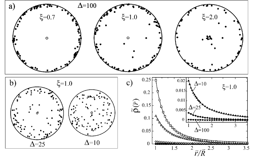
Figure 2: Typical snapshots from the simulations on the counterion-cylinder system in 3D for a) lateral extension parameter $\Delta=\ln(D/R)=100$ and three different Manning parameters $\xi=0.7,1.0$ and 2.0 as indicated on the graph, and b) for Manning parameter $\xi=1.0$ and smaller lateral extension parameters $\Delta=10$ and 25. The snapshots show top-views of the simulation box (see Section V.2 and Figure 1) with radial distances shown in logarithmic scale $y=\ln({\tilde{r}}/{\tilde{R}})$. Point-like counterions are shown by black spheres and the charged cylinder by a circle in the middle. Figure c) gives the simulated radial density of counterions in rescaled units, $\tilde{\rho}(\tilde{r})=\rho(r)/(2\pi\ell_{\mathrm{B}}\sigma_{\mathrm{s}}^{2})$, as a function of the (linear) distance from the cylinder axis. Main set shows the data for $\Delta=100$ and Manning parameters $\xi=2.0$ (open square), 1.5 (open triangle-ups), 1.1 (open diamonds), 1.0 (filled squares) and 0.7 (filled circles) from top to bottom. Inset shows the same for $\xi=1.0$, but for various lateral extension parameters $\Delta=$10, 25 and 100 (top to bottom). Solid curves represent the mean-field PB prediction Eq. (36). Number of counterions here is $N=100$ and the coupling parameter $\Xi=0.1$. Error-bars are smaller than the size of symbols.

V.2 Simulation model and parameters

The geometry of the counterion-cylinder system in our simulations is similar to what we have sketched in Figure 1. We use typically between $N=25$ to 300 counterions (most of the results are obtained with $N$=100 and 200 particles) and increase the lateral extension parameter, $\Delta=\ln(D/R)$, up to $\Delta=300$. We also vary the Manning parameter, $\xi$, and consider a wide range of values for the electrostatic coupling parameter, $\Xi$, from $\Xi=0.1$ (close to the mean-field regime) up to $\Xi=10^{5}$ (close to the strong-coupling regime).

The cylindrical simulation box has a finite height, ${\tilde{L}}$, which is set by the electroneutrality condition (11), i.e. ${\tilde{L}}=N\Xi/\xi$. In order to mimic the thermodynamic limit and reduce the finite-size effects due to the finiteness of the cylinder height, we apply periodic boundary conditions in $z$ direction (parallel to the cylinder axis) by replicating the main simulation box infinitely many times in that direction. The long-range character of the Coulomb interaction in such a periodic system leads to summation of infinite series over all periodic images. These series are not generally convergent, but in an electroneutral system, the divergencies cancel and the series can be converted to fast-converging series. We use the summation techniques due to Lekner Lekner and Sperb Sperb , which are utilized to the one-dimensionally periodic system considered here–see Appendix D (similar methods are developed in Ref. Arnold ). Finally in order to obtain reliable values for the error-bars, the standard block-averaging scheme is used Block_Average . The simulations typically run for $\sim 1.1\times 10^{6}$ Monte-Carlo steps per particle with $\sim 10^{5}$ steps used for the equilibration purpose.

VI Simulation results in 3D

VI.1 Overall behavior in the infinite-system-size limit

VI.1.1 Distribution of counterions

Let us start with the distribution of counterions as generated by the centrifugal sampling method. In Figure 2 typical simulation snapshots are shown together with the counterionic density profile for small coupling parameter $\Xi=0.1$. Counterion distribution is shown for large ($\Delta=100$), intermediate ($\Delta=25$) and small ($\Delta=10$) lateral extension parameter. The counterion-condensation transition is clearly reproduced for large $\Delta$ (Figure 2a): counterions are “de-condensed” and gather at the outer boundary at small Manning parameter (shown for $\xi=0.7$), while they partially “condense” and accumulate near the cylinder surface for large Manning parameter (shown for $\xi=2$). The Manning parameter $\xi=1$, as seen, represents an intermediate situation. This trend is demonstrated on a quantitative level by the radial density profile of counterions $\tilde{\rho}(\tilde{r})$ (Figure 2c, main set), which tends to zero by decreasing $\xi$ down to about unity. Note that relatively large fluctuations occur at low $\xi$ making $\tilde{\rho}(\tilde{r})$ an inconvenient quantity to precisely locate the critical value $\xi_{c}$, which will be considered later. The data moreover follow the mean-field PB density prediction, Eq. (36), shown by solid curves, as expected since the chosen coupling parameter is small.

The transition regime at intermediate $\xi$ exhibits strong finite-size effects. As may be seen from the snapshots in Figure 2b, the de-condensation process at $\xi=1$ is strongly suppressed for small logarithmic sizes $\Delta=\ln(D/R)=10$ and 25. The corresponding density profiles (inset of Figure 2c) indicate a sizable accumulation of counterions near the cylinder surface, which is washed away only by taking a sufficiently large $\Delta$. Such finite-size effects at low $\xi$ are also observed in previous numerical studies, which have devised simulations in linear scale and thus considered only small confinement volumes per polymer (typically $\Delta<10$) Deserno00 ; Liao03 ; Bratko82 ; Zimm84 ; Rossky85 . In some studies Rossky84 , these effects have been interpreted as an evidence for counterion condensation at small $\xi$, leading to the incorrect conclusion that no condensation transition exists.

VI.1.2 Condensed fraction of counterions

Our results for large $\xi$ exhibit a counterionic density profile that extends continuously from the cylinder surface to larger distances. This indicates that making a distinction between two layers of condensed and de-condensed counterions, in the sense of two-fluid models frequently used in literature Manning69 ; Oosawa ; Oosawa_Imai ; Manning77 ; Manning_Dyn ; Manning_rev78 ; Manning_rev96a ; Manning_rev96b ; de-la-Cruz95 ; Levin97 ; Levin98 ; Schiess98 ; Nyquist99 ; Ray_Mann99 ; Henle04 ; Muthu04 , requires a criterion.

The two-fluid description predicts a fraction of

$$\alpha_{\mathrm{M}}=\left\{\begin{array}[]{ll}0&{\,\,\,\,\xi\leq 1}\\ \\ 1-1/\xi&{\,\,\,\,\xi\geq 1}\end{array}\right.$$ (99)

of counterions to reside in the condensed layer (which is considered as a layer with small thickness at the polymer surface), when the infinite-dilution limit is reached. Previous studies Macgillivray ; Ramanathan ; Ramanathan_Wood82a ; Zimm ; Deserno00 ; Shaugh show that the Manning condensed fraction, $\alpha_{\mathrm{M}}$, may also be identified systematically within the Poisson-Boltzmann theory by employing an inflection-point criterion Deserno00 ; Shaugh . This can be demonstrated using the PB cumulative density (the number of counterions inside a cylindrical region of radius $r$), $n_{\mathrm{PB}}(r)$, obtained as

$$\frac{n_{\mathrm{PB}}(r)}{N}=\frac{2\pi L}{N}\int_{R}^{r}r^{\prime}\,{\mathrm{d}}r^{\prime}\,\rho_{\mathrm{PB}}(r^{\prime})=$$

$$=\frac{1}{\xi}\times\left\{\begin{array}[]{ll}(\xi-1)-\beta\coth\bigg{[}\beta y+\coth^{-1}\frac{\xi-1}{\beta}\bigg{]}&{\xi\leq\Lambda_{\mathrm{AF}},}\\ (\xi-1)-\beta\cot\bigg{[}\beta y+\cot^{-1}\frac{\xi-1}{\beta}\bigg{]}&{\xi\geq\Lambda_{\mathrm{AF}},}\end{array}\right.$$ (102)

using Eq. (36). For $\xi\geq\Lambda_{\mathrm{AF}}$, $n_{\mathrm{PB}}(r)$ exhibits an inflection point at a radial distance $r_{\ast}$ when plotted as a function of $y=\ln(r/R)$ Deserno00 . One can show that for $\Delta\rightarrow\infty$, only the fraction of counterions, that lie within the cylindrical region $r\leq r_{\ast}$, remains associated with the cylinder and tends to the Manning condensed fraction, i.e.

$$\frac{n_{\mathrm{PB}}(r_{\ast})}{N}\rightarrow\alpha_{\mathrm{M}}.$$ (103)

In other words, only this fraction of counterions contribute to the asymptotic density profile and the rest ($1/\xi$ of all) is pushed to infinity (Appendix C.4).

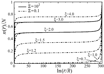
Figure 3: Cumulative density, $n({\tilde{r}})$, per total number $N$, of counterions as a function of the logarithmic distance from the charged cylinder, $\ln({\tilde{r}}/{\tilde{R}})$. Dot-dashed curves are simulation results for $\Xi=0.1$, $N=70$, and $\Delta=300$ and for various Manning parameters as shown on the graph. These curves also closely represent the PB prediction (102), which are not explicitly shown. Solid curves show the simulation data for large coupling parameter $\Xi=10^{2}$ and for $\xi=3.0$ and $\xi=2.0$.

The simulations results for the cumulative density as a function of the logarithmic radial distance $y=\ln(\tilde{r}/\tilde{R})$ are shown in Figure 3 for various Manning parameters (solid and dot-dashed curves). Here we have chosen a very large lateral extension parameter $\Delta=\ln(D/R)=300$, which exhibits the concept of condensed fraction more clearly. The data show an inflection point, which is located approximately at $y_{\ast}=\ln(r_{\ast}/R)\simeq\Delta/2$ for large $\xi$ (for small $\xi\rightarrow 1$, the location of the inflection point, $r_{\ast}$, tends to $R$–see Appendix C.2). The rapid increase of $n(\tilde{r})$ at small ($r\sim R$) and at large distances ($r\sim D$) reflects the two counterion-populated regions at the inner and outer boundaries, which are separated by an extended plateau (compare with Figure 2). For small $\Delta$, the inflection point has a non-vanishing slope and the two regions are not quite separated (data not shown) Deserno00 ; Henle04 (see Ref. Ray_Mann99 for a similar trend in an extended two-fluid model).

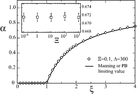
Figure 4: Main set: Simulated condensed fraction of counterions, $\alpha$, as defined via the inflection-point criterion, as a function of Manning parameter, $\xi$, for $\Xi=0.1$ (diamonds). Solid curve displays Manning (or the PB) limiting value, $\alpha_{\mathrm{M}}$, for $\Delta=\ln(D/R)\rightarrow\infty$ (Eq. (99)). Inset: Condensed fraction as a function of the coupling parameter, $\Xi$, for $\xi=3.0$. These data are obtained for $\Delta=300$ and $N=70$.

Using the inflection-point criterion, the condensed fraction, $\alpha$, may be estimated as $\alpha=n(r_{\ast})/N$ Deserno00 , which roughly corresponds to the plateau level in Figure 3. Simulation results are shown in Figure 4 for large $\Delta=300$. Let us first consider the case of a small coupling parameter $\Xi=0.1$, where the simulated cumulative density, $n(\tilde{r})$ (dot-dashed curves in Figure 3), closely follows the PB prediction (102) (PB curves are not explicitly shown). The calculated condensed fraction (diamonds in Figure 4) agrees already quite well (within $<1$%) with the Manning or PB limiting value $\alpha_{\mathrm{M}}$ (solid curve in Figure 4).

An important question is whether the form of the cumulative density profile, $n(\tilde{r})$, and the condensed fraction are influenced by electrostatic correlations for increasing coupling parameter $\Xi$. In Figure 3, we show $n(\tilde{r})$ from the simulations for $\Xi=10^{2}$ and for two values of Manning parameter $\xi=2.0$ and 3.0 (solid curves). This coupling strength generally falls into the strong-coupling regime for charged systems, where electrostatic correlations are expected to matter Naji_PhysicaA (note that DNA with trivalent counterions represents $\Xi\sim 10^{2}$, but with a larger $\xi\sim 12$). As seen, $n(\tilde{r})$ shows a more rapid increase at small distances from the cylinder (condensed region) indicating a stronger accumulation of counterions near the surface. This trend is also observed in previous simulations Deserno00 ; Zimm84 ; Bratko82 ; Rossky85 and in experiments with multivalent counterions Zakha99 , and will be analyzed in more detail in the following sections.

However, in contrast to previous conclusions (obtained based on small values of $\Delta$) Deserno00 ; Henle04 , the aforementioned behavior for large $\Xi$ does not imply a larger condensed fraction as defined within the inflection-point criterion. Since as seen in Figure 3, the large-distance behavior of the density profile is not influenced by electrostatic correlations, and so remains the condensed fraction (plateau level) unaffected for increasing coupling strength (inset of Figure 4). This result can be appreciated only when the asymptotic behavior for $\Delta\gg 1$ is considered.

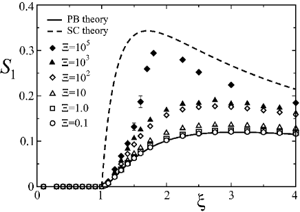
Figure 5: Simulation data for the order parameter $S_{1}=\langle 1/{\tilde{r}}\rangle$ as a function of Manning parameter, $\xi$, for various coupling parameters $\Xi=0.1$ up to $10^{5}$ as indicated on the graph. The mean-field PB and the strong-coupling predictions are calculated from Eqs. (52) and (91) (solid and dashed curves respectively). The lateral extension parameter is $\Delta=300$ and the number of counterions is $N=200$ for $\Xi=0.1$, $N=50$ for $\Xi=10^{5}$, and $N=70$ for other coupling parameters.

VI.1.3 The order parameters $S_{n}$

The $n$-th-order inverse moment of the counterionic density profile may be calculated numerically using

$$S_{n}=\frac{1}{N}\sum_{i=1}^{N}{\overline{{\tilde{r}}_{i}^{-n}}}$$ (104)

for $n>0$, where ${\tilde{r}}_{i}$ is the radial distance of the $i$-th counterion from the cylinder axis and the bar sign denotes the Monte-Carlo time average after proper equilibration of the system. The overall behavior is shown in Figure 5 for $S_{1}$ as a function of Manning parameter, $\xi$. Recall that a vanishing order parameter, $S_{1}$, indicates the complete de-condensation of counterions, while a finite $S_{1}$ reflects a finite degree of counterion binding to the charged cylinder (corresponding to a finite localization length $\sim 1/S_{1}$).

As seen from the figure, de-condensation can occur in all relevant regimes of the coupling parameter $\Xi$. For large Manning parameter, electrostatic coupling effects become important and shift the order parameter to larger values exhibiting a crossover from the mean-field prediction (solid curve), which is verified for small $\Xi<1$, to the strong-coupling prediction (dashed curve) at very large values of $\Xi$ Netz ; Andre ; Naji04 . The mean-field result follows from Eq. (52) and the strong-coupling prediction is obtained using Eq. (91). As seen, in the transition regime $\xi\sim 1$, the order parameter data remain close to the mean-field curve and deviate from the SC prediction. A close examination of correlation effects as well as finite-size effects in this region is quite important in determining the scaling behavior and will be considered later. Here we concentrate on the correlation-induced crossover behavior in the condensation phase.

VI.1.4 Electrostatic correlations at surface and for large $\xi$

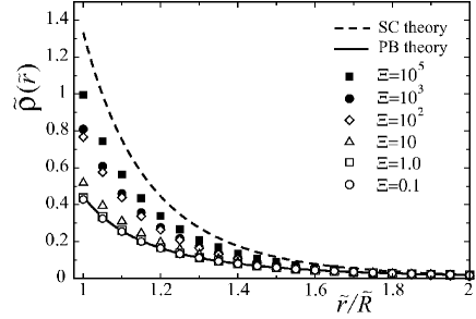
Figure 6: Radial density of counterions in rescaled units, $\tilde{\rho}(\tilde{r})=\rho(r)/(2\pi\ell_{\mathrm{B}}\sigma_{\mathrm{s}}^{2})$, as a function of the (linear) distance from the cylinder axis for Manning parameter $\xi=3.0$ and various coupling parameters ($\Xi=0.1$ up to $10^{5}$) as shown on the graph. Here $\Delta=300$ and the number of counterions is $N=50$ for $\Xi=10^{5}$, and $N=70$ for other values of $\Xi$. The mean-field (solid curve) and the strong-coupling (dashed curve) predictions are obtained from Eqs. (36) and (87), which, for $\Delta=300$, roughly coincide with the asymptotic expressions (46) and (89).

In Figure 6, we plot the simulated radial density profile of counterions, $\tilde{\rho}({\tilde{r}})$, for $\xi=3.0$ and consider several different coupling parameters. In agreement with the preceding results, the counterionic density in the immediate vicinity of the charged cylinder increases for increasing $\Xi$ exhibiting large deviations from the mean-field prediction (see Ref. Lau_Safran for a similar trend at charged plates). For a given surface charge density $\sigma_{\mathrm{s}}$, the observed trend is predicted, e.g., for increasing counterion valency, $q$, since the coupling parameter scales as $\Xi\sim q^{3}$ (Eq. (8)). The crossover from the mean-field PB prediction (solid curve) to the strong-coupling prediction (dashed curve) appears to be quite weak, in agreement with the situation observed for counterions at planar charged walls Andre . These limiting profiles are calculated from Eqs. (36) and (87) respectively, and both exhibit an algebraic decay with the radial distance, $\tilde{r}$. But the SC profile shows a faster decay and thus a more compact counterion layer near the surface at large coupling strength (compare Eqs. (46) and (89)).

An interesting point is that the simulated density at contact with the cylinder shows a more rapid increase when the coupling parameter increases from $\Xi=10$ to $\Xi=100$ as compared with other ranges of $\Xi$ (Figure 6). This is in fact accompanied by the formation of correlation holes around counterions near the surface as we show now.

In order to examine counterion-counterion correlations at the surface, we consider the one-dimensional pair distribution of counterions, $g_{\mathrm{1D}}({\tilde{z}})$, which measures the probability of finding two counterions lined-up along $z$-axis (i.e. along the cylinder axis with equal azimuthal angles $\phi$) at a distance ${\tilde{z}}$ from each other. In Figure 7, we plot the unnormalized pair distribution function defined via

$$g_{\mathrm{1D}}({\tilde{z}})\equiv\frac{1}{N}\sum_{i\neq j}^{\prime}\bigg{\langle}\delta({\tilde{z}}_{i}-{\tilde{z}}_{j}-{\tilde{z}})\,\delta(\phi_{i}-\phi_{j})\bigg{\rangle},$$ (105)

where the prime mark indicates that the sum runs only over counterions at the surface (defined in the simulations as counterions residing in a shell of thickness about the Gouy-Chapman length, $\mu$, around the cylinder). At small coupling parameter ($\Xi=10$, cross symbols), the pair distribution function only shows a very weak depletion zone at small distances along the cylinder axis. For larger values of $\Xi$, one observes a pronounced correlation hole at small distances around counterions, where the distribution function vanishes over a finite range. This correlation hole develops in the range of coupling parameters $10<\Xi<100$, which marks the crossover regime between the mean-field and the strong-coupling regime (compare cross symbols and filled triangle-ups) Andre . The correlation hole appears only for sufficiently large Manning parameter $\xi$ (large enough number of condensed counterions) and is distinguishable in our simulations for $\xi>1.2$.

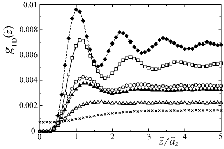
Figure 7: The one-dimensional pair distribution function of counterions at contact with cylinder as defined in Eq. (105). Symbols show simulation data for $\Xi=10^{5}$ and $\xi=4.0$ (filled diamonds), $\Xi=10^{3}$ and $\xi=2.0,3.0$ and 4.0 (open symbols from bottom to top), and for coupling parameters $\Xi=10$ and $\Xi=100$ with Manning parameter $\xi=3.0$ (cross symbols and filled triangle-ups respectively).

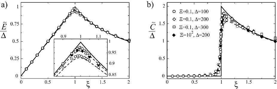
Figure 8: a) The rescaled internal energy, ${\tilde{E}}=E_{N}/(Nk_{\mathrm{B}}T)$ and b) the rescaled excess heat capacity, ${\tilde{C}}=C_{N}/(Nk_{\mathrm{B}})$, of the counterion-cylinder system as a function of Manning parameter, $\xi$. Open symbols show the data for small coupling parameter $\Xi=0.1$ and for increasing lateral extension parameters $\Delta=100,200$ and 300 as indicated on the graph. Filled symbols are the data for large coupling $\Xi=10^{2}$ and $\Delta=200$. Here number of counterions is $N=100$. Solid curves show the asymptotic PB prediction for $\Delta\rightarrow\infty$, Eqs. (82) and (86). Dashed curves are the full PB result for $\Delta=100$ and 300 (from bottom to top), which are calculated numerically using Eqs. (74) and (110). The inset shows a closer view of the energy peak.

The small-separation correlation hole is followed by an oscillatory behavior for elevated $\xi$ indicative of a short-ranged liquid-like order among counterions line-up along the cylinder axis (distinguishable from the data for $\xi>2.0$ in the large-coupling regime $\Xi>100$). The location of the first peak of $g_{\mathrm{1D}}$ gives a rough measure of the typical distance between lined-up counterions, $a_{z}$, at the cylinder surface. This distance is set by the local electroneutrality condition $a_{z}\tau=q$. In rescaled units, we obtain

$${\tilde{a}_{z}}\equiv\frac{a_{z}}{\mu}=\frac{\Xi}{\xi},$$ (106)

from Eqs. (5), (6) and (8), which is used to rescale the horizontal axis of the graph in Figure 7.

Note that the correlation hole size increases with the coupling parameter and thus counterions at the surface become highly isolated, reflecting dominate single-particle contributions for $\Xi\gg 1$ Netz ; Andre . In fact, as discussed elsewhere Netz ; Andre ; Naji04 ; Naji_PhysicaA ; Burak04 , the single-particle form of the SC theory (obtained formally for $\Xi\rightarrow\infty$) is a direct consequence of large correlation hole size around counterions at the surface. Clearly, for the counterion-cylinder system, this can be the case only for sufficiently large Manning parameter, where a sizable fraction of counterions can gather near the surface. Consequently in this regime, the data tend to the strong-coupling predictions for elevated $\Xi$ (Figures 5 and 6) as also verified in the simulations of charged plates, where all counterions are bound to the surface Andre , and two charged cylinders with large $\xi$ Naji04 . This also explains why the SC theory, though being able to reproduce the CCT on a qualitative level, fails to capture the quantitative features near the critical point (except for the value of the critical Manning parameter), where counterion are mostly de-condensed.

VI.2 Critical Manning parameter $\xi_{c}$

We now turn our attention to the behavior of counterions near the critical point and begin with determining the precise location of the critical Manning parameter, $\xi_{c}$.

To this end, we shall employ a procedure similar to the method of locating the transition temperature in bulk critical phenomena critical ; Landau91 . Namely, one expects that the transition point is reflected by a singular behavior in thermodynamic quantities such as energy or heat capacity as already indicated by the mean-field results obtained in Section III.3.2. The mean (internal) energy, $E$, and the excess heat capacity, $C$, may be obtained directly from the simulations and in rescaled units as

$${\tilde{E}}=\frac{E_{N}}{Nk_{\mathrm{B}}T}=\bigg{\langle}\frac{{\mathcal{H}}_{N}}{Nk_{\mathrm{B}}T}\bigg{\rangle},$$ (107)

$${\tilde{C}}=\frac{C_{N}}{Nk_{\mathrm{B}}}=N\bigg{\langle}\left(\frac{{\delta\mathcal{H}}_{N}}{Nk_{\mathrm{B}}T}\right)^{2}\bigg{\rangle},$$ (108)

where the configurational Hamiltonian ${\mathcal{H}}_{N}$ is defined through Eq. (10) and $\delta{\mathcal{H}}_{N}={\mathcal{H}}_{N}-\langle{\mathcal{H}}_{N}\rangle$.

Simulation results for the rescaled energy, $\tilde{E}$, and the rescaled excess heat capacity, $\tilde{C}$, in Figure 8 (symbols) show a non-monotonic behavior as a function of $\xi$. The energy develops a pronounced peak and the heat capacity exhibits a jump at intermediate Manning parameters, which become singular for $\Delta$ increasing to infinity. The general behavior of energy and heat capacity can be understood using simple arguments as follows.

For sufficiently small $\xi$, counterions are all unbound and the electrostatic potential in space is roughly given by the bare potential of the charged cylinder, i.e. $\psi({\tilde{r}})\simeq 2\xi\ln({\tilde{r}}/\tilde{R})$. This yields the rescaled internal energy, $\tilde{E}$, (via integrating over the square electric field, Eq. (70)) as

$$\tilde{E}=\frac{1}{4\xi}\int_{\tilde{R}}^{\tilde{D}}\,\tilde{r}\,{\mathrm{d}}\tilde{r}\,\bigg{(}\frac{{\mathrm{d}}\psi}{{\mathrm{d}}\tilde{r}}\bigg{)}^{2}\simeq\xi\Delta$$ (109)

for $\Delta=\ln(D/R)\gg 1$. Intuitively, this result may be obtained also by assuming that counterions experience the potential of the cylinder at the outer boundary; thus one simply has $\tilde{E}\simeq\psi(\tilde{D})/2\simeq\xi\Delta$, which explains the linear increase of the left tail of the energy curve with both $\xi$ and $\Delta$ (Figure 8a). Now using the following thermodynamic relation

$$\xi\frac{\partial\tilde{E}}{\partial\xi}={\tilde{E}}-{\tilde{C}},$$ (110)

the excess heat capacity is obtained to vanish in the de-condensation regime, i.e. $\tilde{C}\simeq 0$ (Figure 8b). Hence, the heat capacity reduces to that of an ideal gas of particles.

For large $\xi$, the electrostatic potential of the cylinder is screened due to counterionic binding. If we estimate the screened electrostatic potential of the cylinder as $\psi({\tilde{r}})\simeq 2\ln({\tilde{r}}/{\tilde{R}})$, which can be verified systematically within the PB theory Fuoss51 ; Netz_Joanny , we obtain the energy and the heat capacity as

$$\tilde{E}\simeq\Delta/\xi\,\,\,\,{\mathrm{and}}\,\,\,\,\tilde{C}\simeq 2\Delta/\xi.$$ (111)

These results may also be obtained by noting that only the fraction $1/\xi$ of de-condensed counterions (Section VI.1.2) contributes to the energy on the leading order; thus $\tilde{E}\simeq\psi(\tilde{D})/(2\xi)\simeq\Delta/\xi$. The above asymptotic estimates in fact coincide with the asymptotic ($\Delta\rightarrow\infty$) PB results (82) and (86), which are shown by solid curves in Figure 8.

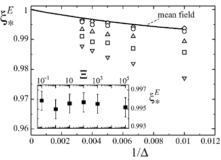
Figure 9: Main set: Location of the peak of energy, $\xi_{\ast}^{E}$, as a function of the inverse lateral extension parameter, $1/\Delta=1/\ln(D/R)$. Open symbols are simulation results for small coupling parameter $\Xi=0.1$ and for various number of counterions (from bottom): $N=25$ (triangle-downs), 50 (squares), 100 (triangle-ups), 200 (circles) and 300 (diamonds). Solid curve shows the mean-field PB prediction for the peak location as obtained by numerical evaluation of the full PB energy, Eq. (74). Inset: Location of the energy peak as a function of the coupling parameter, $\Xi$, for $N=200$ and $\Delta=300$.

The preceding considerations demonstrate that the non-monotonic behavior of the energy and excess heat capacity results directly from the screening effect due to the condensation of counterions for increasing $\xi$. Hence, the singular peaks emerging in both quantities reflect the onset of the counterion-condensation transition, $\xi_{c}$, which occurs in the thermodynamic infinite-system-size limit $N\rightarrow\infty$ and $\Delta\rightarrow\infty$. Within the PB theory (solid and dashed curves in Figure 8), the location of the peak of energy, $\xi_{\ast}^{E,{\mathrm{PB}}}(N,\Delta)$, tend to the mean-field critical value $\xi_{c}^{\mathrm{PB}}=1$ from below as $\Delta$ increases obeying the finite-size-scaling relation

$$\xi_{c}^{\mathrm{PB}}-\xi_{\ast}^{E,{\mathrm{PB}}}(\Delta)\simeq\frac{1}{\Delta},$$ (112)

which is obtained using the full PB energy (74). On the other hand, the location of the peak of the PB heat capacity approaches $\xi_{c}^{\mathrm{PB}}$ from above.

We locate the critical point from the asymptotic behavior of the energy peak, $\xi_{\ast}^{E}$, for increasing $N$ and $\Delta$. (The heat capacity peak is found to be located further away from the critical point than the energy peak, resembling the well-known behavior of the heat capacity peak in finite Magnetic systems Landau91 , which makes it inconvenient for our purpose). In Figure 9, we show the simulation results for $\xi_{\ast}^{E}$ (symbols) as a function of $\Delta^{-1}$ for $\Xi=0.1$ and for various number of particles (main set). These data are obtained using the thermodynamic relation (110), which allows us to calculate the first derivative of energy, $\partial\tilde{E}/\partial\xi$, directly from the energy and the heat capacity data without referring to numerical differentiation methods which typically generate large errors near the peak. As seen, for increasing $N$, the data converge to and closely follow the mean-field prediction (solid curve) within the estimated error-bars; for $N>100$, $\xi_{\ast}^{E}$ lies within about 1% of the PB critical Manning parameter $\xi_{c}^{\mathrm{\mathrm{PB}}}=1$. Since in the simulations we have used $\Delta\leq 300$, the behavior of $\xi_{\ast}^{E}$ for very small $\Delta^{-1}\rightarrow 0$ is not obtained, nevertheless, the excellent convergence of the data for $\Xi=0.1$ to the PB prediction gives an accurate estimate for the critical Manning parameter as

$$\xi_{c}=1.00\pm 0.002.$$ (113)

Our results for larger values of the coupling parameter, $\Xi$, in the inset of Figure 9 show that the location of the energy peak does not vary with the coupling parameter. Therefore, we find that the critical Manning parameter is universal and given by the mean-field value $\xi_{c}=1.0$. Recall that the same threshold is obtained within the Onsager instability and the strong-coupling analysis (Sections II.5 and IV).

Another important result is that the CCT is not associated with a diverging singularity, in contrast to the Onsager instability prediction Manning69 . But, the energy at any finite value of $\xi$, and also the heat capacity for $\xi>1$, tend to infinity (as $\sim\Delta$) when the lateral extension parameter, $\Delta$, increases to infinity, which, as illustrated before, reflects the logarithmic divergency of the effective electrostatic potential in a charged cylindrical system. The CCT, however, exhibits a universal discontinuous jump for the excess heat capacity at $\xi_{c}$, and thus indicates a second-order phase transition (Figure 8).

VI.3 Scale-invariance near the critical point

Now that the precise location of the critical Manning parameter is determined, a finite-size analysis, similar to what we presented within the mean-field theory, may be used to determine the near-threshold properties of the CCT order parameters from the simulation data.

Note that in the simulations, finite size effects arise both from the finiteness of the system size (via the lateral extension parameter, $\Delta$), and also from the finiteness of the number of counterions, $N$; the latter being related to the finiteness of the height of the main simulation box $L=Nq/\tau$ (Section V), which has a sizable influence on the transition, although the implemented periodic boundary condition already reduces its effects. In what follows, we present the numerical evidence for scaling relations with respect to both $N$ and $\Delta$. The asymptotic behavior for increasing $N$ and $\Delta$ to infinity provides us with the scaling behavior with respect to the reduced Manning parameter, $\zeta$ (or the reduced temperature, $t$), which characterizes the CCT universality class in 3D.

VI.3.1 Finite-size effects near $\xi_{c}$

In Figure 10 (main set), we show the order parameter $S_{1}$ as a function of $1/\Delta$ and in the vicinity of the critical point $\xi_{c}=1$ (number of counterions $N=100$ is fixed). $S_{1}$, which represents the mean inverse localization length of counterions, gradually decreases with decreasing $1/\Delta$ as de-condensation of counterions becomes gradually more pronounced, but for Manning parameters as large as $\xi=1.05$ (open circles), the data quickly saturate to a finite value as $\Delta\rightarrow\infty$. For sufficiently small Manning parameter (e.g., $\xi<0.97$), on the other hand, $S_{1}$ converges to zero. In the vicinity of the critical point ($\xi=1$, diamonds), a non-saturating behavior is found suggesting a power-law decay as $S_{1}\sim\Delta^{-\gamma}$, where $\gamma>0$. As seen, the data at $\xi=1$ roughly coincide for both small coupling ($\Xi=0.1$, open diamonds) and large coupling ($\Xi=10^{2}$, filled diamonds) indicating that electrostatic correlations do not influence the scaling behavior (see below). There still remain non-negligible deviations between the simulation data at the critical point (diamonds) and the PB power-law prediction (57) with $\gamma_{\mathrm{PB}}=2$, which is shown in the figure by a straight dot-dashed line. These deviations arise from the finiteness of the number of particles.

Interestingly, the data obtained for increasing number of counterions, $N$ (at fixed lateral extension parameter, $\Delta$), also indicate a power-law decay near the critical point, i.e. as $S_{1}\sim N^{-\nu}$, where $\nu>0$. This is shown in the inset of Figure 10, where the scaling exponent $\nu$ appears to be about $2/3$ (represented by a dashed line). In fact, for sufficiently large $N$, the data deviate from this power-law behavior since finite-size effects due to lateral extension of the system, $\Delta$, are simultaneously present. Thus in order to determine the exponents $\gamma$ and $\nu$, a more systematic approach is required, which should incorporate both lateral-size and ion-number effects.

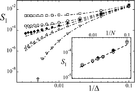
Figure 10: Main set: Order parameter $S_{1}=\langle 1/\tilde{r}\rangle$ as a function of the inverse lateral extension parameter $1/\Delta$. Open symbols are data for $\Xi=0.1$ and Manning parameters (from top): $\xi=1.05$ (squares), 1.01 (circles), 1.0 (open diamonds), 0.99 (triangle-ups) and 0.97 (triangle-downs). Filled diamonds are the data for large coupling parameter $\Xi=10^{2}$ and $\xi=1.0$. Number of counterions $N=100$ is fixed. Dot-dashed curves are the PB result, Eq. (52), for the corresponding $\xi$. Inset: $S_{1}$ as a function of the inverse number of counterions $1/N$ for $\xi=1.0$ and for the coupling parameters $\Xi=0.1$ (open diamonds), $10^{2}$ (filled diamonds) and $10^{3}$ (open circles). Dashed line shows the power-law exponent 2/3. Here $\Delta=300$.

VI.3.2 Generalized finite-size scaling relations

In brief, our data suggest that at the critical point ($\zeta=1-\xi_{c}/\xi=0$) and for a bounded system (finite $\Delta$) in the thermodynamic limit $N\rightarrow\infty$, the order parameter $S_{n}(\zeta,\Delta,N)=\langle 1/\tilde{r}^{n}\rangle$ decays as

$$S_{n}(0,\Delta,\infty)\sim\Delta^{-\gamma},$$ (114)

while in an unbounded system ($\Delta\rightarrow\infty$) and for finite $N$, we expect a power-law decay as

$$S_{n}(0,\infty,N)\sim N^{-\nu}.$$ (115)

In thermodynamic infinite-system-size limit ($\Delta\rightarrow\infty$ and $N\rightarrow\infty$), the true critical transition sets in with $S_{n}(\zeta<0,\infty,\infty)=0$, and we anticipate the scaling behavior with the reduced Manning $\zeta$ as

$$S_{n}(\zeta,\infty,\infty)\sim\zeta^{\chi}$$ (116)

in a sufficiently small neighborhood above $\xi_{c}=1$.

These scaling relations may all be deduced from a general finite-size scaling hypothesis for $S_{n}$, i.e. assuming that $S_{n}(\zeta,\Delta,N)$ takes a homogeneous scale-invariant form with respect to its arguments in the vicinity of the transition point, $\xi_{c}$, when both $N$ and $\Delta$ are sufficiently large. In other words, for any positive number $\lambda>0$,

$$S_{n}(\lambda\zeta,\lambda^{-b}\Delta,\lambda^{-c}N)=\lambda^{a}S_{n}(\zeta,\Delta,N),$$ (117)

where $a,b$ and $c$ are a new set of exponents associated with $\zeta,\Delta$ and $N$ respectively. The above relation implies that when the reduced Manning parameter, $\zeta$, is rescaled with a factor $\lambda$, the size parameters, $N$ and $\Delta$, can be rescaled such that the order parameter remains invariant up to a scaling prefactor. Finite-size scale-invariance is a common feature in critical phase transitions critical ; Fisher72 and provides an accurate tool to estimate critical exponents in numerical simulations Landau91 ; Binder88 . The exponents in Eq. (117) can be calculated directly from MC simulations. These exponents are in fact related to and give the values of the desired critical exponents $\gamma$, $\nu$ and $\chi$, as will be shown below. Note that the exponents may in general depend on $n$ (the index of $S_{n}$), the coupling parameter, $\Xi$, or the space dimensionality, which are not explicitly incorporated in the proposed scaling hypothesis, but their influence will be examined later.

Given Eq. (117), the following relations are obtained by suitably choosing $\lambda$. For $\lambda=N^{1/c}$, one finds

$$S_{n}(\zeta,\Delta,N)=N^{-a/c}{\mathcal{C}}_{n}(\zeta N^{1/c},\Delta N^{-b/c}),$$ (118)

where ${\mathcal{C}}_{n}(u,v)$ is the scaling function corresponding to a system with both finite $N$ and $\Delta$. The above expression is useful for a system with finite $N$ in the limit $\Delta\rightarrow\infty$. Thus assuming that ${\mathcal{C}}_{n}(u,v)$ exists for $v=\Delta N^{-b/c}\rightarrow\infty$, the relation (118) reduces to

$$S_{n}(\zeta,\infty,N)=N^{-a/c}{\mathcal{N}}_{n}(\zeta N^{1/c}),$$ (119)

where the scaling function ${\mathcal{N}}_{n}(u)={\mathcal{C}}_{n}(u,\infty)$. The critical exponent $\nu$ follows by considering this relation right at the critical point, $\zeta=0$, i.e.

$$S_{n}(0,\infty,N)={\mathcal{N}}_{n}(0)\,N^{-\nu},$$ (120)

where $\nu$ is obtained as

$$\nu=\frac{a}{c}.$$ (121)

On the other hand, we assume that in the vicinity of (and above) the critical point (i.e. for small but finite $\zeta$), $S_{n}(\zeta,\infty,N)$ is only a finite function of the reduced Manning parameter $\zeta$ when the limit $N\rightarrow\infty$ is taken. Hence the scaling function ${\mathcal{N}}_{n}(u)$ is required to behave as ${\mathcal{N}}_{n}(u)\sim u^{a}$ for $u\rightarrow\infty$, which yields

$$S_{n}(\zeta,\infty,\infty)\sim\zeta^{\chi},$$ (122)

where the critical exponent associated with $\zeta$ reads

$$\chi=a.$$ (123)

To determine the critical exponent associated with $\Delta$ in terms of the exponents $\{a,b,c\}$, we need to consider Eq. (117) for $\lambda=\Delta^{1/b}$. We thus have

$$S_{n}(\zeta,\Delta,N)=\Delta^{-a/b}{\mathcal{C}^{\prime}}_{n}(\zeta\Delta^{1/b},N\Delta^{-c/b}),$$ (124)

where ${\mathcal{C}^{\prime}}_{n}(u,v)$ is a new scaling function. This relation is useful for a system with finite $\Delta$ in the limit $N\rightarrow\infty$, where assuming that ${\mathcal{C}^{\prime}}_{n}(u,v)$ exists, we obtain

$$S_{n}(\zeta,\Delta,\infty)=\Delta^{-a/b}{\mathcal{D}}_{n}(\zeta\Delta^{1/b})$$ (125)

with a new scaling function ${\mathcal{D}}_{n}(u)={\mathcal{C}^{\prime}}_{n}(u,\infty)$. The critical exponent $\gamma$ follows by considering this relation right at the critical point, $\zeta=0$, that yields

$$S_{n}(0,\Delta,\infty)={\mathcal{D}}_{n}(0)\,\Delta^{-\gamma},$$ (126)

where $\gamma$ reads

$$\gamma=\frac{a}{b}.$$ (127)

Therefore, we have a complete set of relations (121), (123) and (127) from which the critical exponents $\gamma$, $\nu$ and $\chi$ may be obtained using the exponents $a,b$ and $c$.

Equation (125) compares directly with the mean-field result, Eq. (57), where we showed that $\gamma_{\mathrm{PB}}=2$ and $\chi_{\mathrm{PB}}=2$. Note also that the exponent $\nu$ is not defined within the mean-field theory.

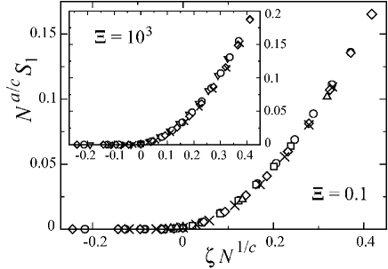
Figure 11: Rescaled order parameter, $N^{a/c}S_{1}$, as a function of the rescaled reduced Manning parameter, $\zeta N^{1/c}$, in the vicinity of the critical point, $\xi_{c}=1.0$, and for small and large coupling parameters $\Xi=0.1$ (main set) and $\Xi=10^{3}$ (inset). Symbols show data for various number of particles $N=50$ (triangle-downs), 70 (circles), 75 (squares), 100 (diamonds), 200 (cross symbols), 300 (triangle-ups), and fixed $\Delta=300$. In these plots, the exponents are chosen here as $a/c=2/3$ and $1/c=1/3$. Error-bars are smaller than the symbol size.

VI.4 Critical exponents: the CCT universality class

VI.4.1 The exponents $\chi$ and $\nu$

In order to verify the generalized finite-size scaling hypothesis (117) and estimate the critical exponents numerically, we shall adopt the standard data-collapse scheme used widely in literature Binder88 .

We begin with the exponents $\chi$ and $\nu$ that can be calculated using Eq. (118), which involves a scaling function, ${\mathcal{C}}_{n}(u,v)$, of two arguments $u=\zeta N^{1/c}$ and $v=\Delta N^{-b/c}$. In our simulations, $N$ ranges from 25 up to 300 and $\Delta$ ranges from 50 up to 300; thus assuming that the exponent $b/c$ is small, which will be verified later on, we deal with a typically large value for $v\sim 10-10^{2}$. Therefore the limiting relation (119) is approximately valid and yields

$$N^{a/c}S_{n}\simeq{\mathcal{N}}_{n}(\zeta N^{1/c}).$$ (128)

Now if the data for $S_{n}$ are plotted as function of $\zeta=1-\xi_{c}/\xi$ for various $N$ (but at fixed sufficiently large $\Delta$), equation (128) predicts that by rescaling the reduced Manning parameter $\zeta$ by the factor of $N^{1/c}$ and the order parameter by the factor $N^{a/c}$, all data should collapse onto a single curve. Numerically, this procedure allows to determine the exponents $a/c$ and $1/c$ in such a way that the best data collapse is achieved. We show the results in Figure 11 for various $N$ (symbols) and for the coupling parameter $\Xi=0.1$ (main set). The collapse of the data onto each other is indeed achieved within the numerical error-bars for the exponents in the range $1/c\simeq 1/3\pm 0.05$ and $a/c\simeq 2/3\pm 0.1$. This yields the critical exponents $\nu$ and $\chi$ from Eqs. (121) and (123) as

$$\nu\simeq 2/3\pm 0.1,$$ (129)

$$\chi\simeq 2.0\pm 0.4,$$ (130)

where the errors are estimated using the standard error propagation methods. The value obtained for $\chi$ agrees with the mean-field result, Eq. (56).

In order to check whether the exponents vary with the electrostatic coupling parameter, $\Xi$, we repeat this procedure for a wide of range of values for $\Xi$. We find the same values for the exponents for coupling parameters up to $\Xi=10^{5}$. For comparison, the results for $\Xi=10^{3}$ are shown in the inset of Figure 11, where the data collapse is demonstrated for $1/c=1/3$ and $a/c=2/3$.

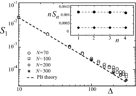
Figure 12: Main set: Order parameter $S_{1}$ as a function of the lateral extension parameter, $\Delta$, for increasing number of counterions from $N=70$ up to 300 as indicated on the graph (Manning parameter here is $\xi=1.0$ and the coupling parameter $\Xi=0.1$). Dashed line shows the PB power-law, Eq. (57). Inset: Rescaled order parameters $S_{n}=\langle\tilde{r}^{-n}\rangle$ as a function of $n$ for Manning parameters close to the critical point (from top): $\xi=1.03$ (filled circles) and $\xi=1.01$ (filled diamond). Here the coupling parameter is $\Xi=0.1$, the number of counterions $N=100$, and $\Delta=300$.

VI.4.2 The exponent $\gamma$

Given the exponents $a$ and $c$ calculated above and making use of the finite-size scaling relation (124), we can estimate the exponent $b$, and thereby the scaling exponent $\gamma$, associated with the lateral extension parameter. In this case, however, the second argument $v=N\Delta^{-c/b}$ in the scaling function ${\mathcal{C}^{\prime}}_{n}(u,v)$ defined in Eq. (124) may not be considered as large within our simulations (since as shown below the ratio $c/b$ is large). But it turns out that the dependence of ${\mathcal{C}^{\prime}}_{n}(u,v)$ on $v$ is quite weak such that the finite-size scaling relation (125) is approximately valid and can thus give the desired exponent. To examine this latter property of ${\mathcal{C}^{\prime}}_{n}(u,v)$, we consider the relation (124) right at the critical Manning parameter ($\zeta=0$), i.e.

$$S_{n}(0,\Delta,N)=\Delta^{-a/b}{\mathcal{C}}_{n}(0,N\Delta^{-c/b}).$$ (131)

In Figure 12, $S_{n}(0,\Delta,N)$ is plotted as a function of $\Delta$ in a log-log plot for increasing $N$ from 70 up to 300 and for $\Xi=0.1$. As clearly seen, the order parameter varies quite weakly with the number of particles, and the variations are already within the error-bars (equal to symbol size) for $N>100$.

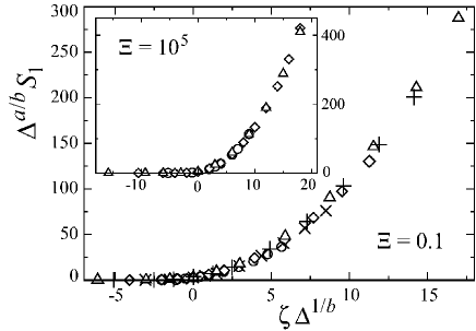
Figure 13: Rescaled order parameter, $\Delta^{a/b}S_{1}$, as a function of the rescaled reduced Manning parameter, $\zeta\Delta^{1/b}$, in the vicinity of the critical point, $\xi_{c}=1.0$, and for small and large coupling parameters $\Xi=0.1$ (main set) and $\Xi=10^{5}$ (inset). Symbols show data for various lateral extension parameters $\Delta=100$ (circles), 150 (cross symbols), 200 (diamonds), 250 (plus symbols) and 300 (triangle-ups). Number of counterions is fixed ($N=200$ for the coupling parameter $\Xi=0.1$ and $N=100$ for $\Xi=10^{5}$), and the exponents are here chosen as $a/b=2.0$ and $1/b=1.0$.

Thus multiplying both sides of Eq. (125) with $\Delta^{a/b}$, we have

$$\Delta^{a/b}S_{n}\simeq{\mathcal{D}}_{n}(\zeta\Delta^{1/b}),$$ (132)

in which the exponent $a$ previously determined as $a=\chi=2.0\pm 0.4$. We thus plot the order parameter $S_{n}$ as a function of $\zeta$ for various $\Delta$ (but at fixed sufficiently large $N$), and rescale both $S_{n}$ and $\zeta$ values with the scaling factors $\Delta^{a/b}$ and $\Delta^{1/b}$ respectively; the exponent $b$ is chosen in such a way that the best data collapse is obtained within the error-bars. The result is shown in Figure 13 for $\Delta^{a/b}S_{1}$ as a function of $\zeta\Delta^{1/b}$, where the coupling parameter is chosen as $\Xi=0.1$. The collapse of the data onto each other is obtained only for the exponent $1/b$ in the range $1/b\simeq 1.0\pm 0.2$, yielding the critical exponent $\gamma$ from Eq. (127) as

$$\gamma\simeq 2.0\pm 0.6,$$ (133)

which agrees with the mean-field exponent, Eq. (59). We find the same value for $\gamma$ by repeating the above procedure for larger coupling parameters. For instance, the results for $\Xi=10^{5}$ are shown in the inset of Figure 13, where we have chosen $1/b=1.0$.

Note that the estimated values of $b$ and $c$ show that the ratio $b/c$ is as small as 0.3, which is consistent with the assumption made in using the asymptotic forms (119) and (125) in the foregoing data-collapse procedure.

As a main result, our numerical data confirm the existence of characteristic scaling relations associated with the counterion-condensation transition in 3D and show that the values of the critical exponents are universal, i.e. independent of the coupling parameter, $\Xi$, and agree with the mean-field universality class.

Also, in agreement with mean-field results, the exponents are found to be independent of $n$, the index of the order parameters $S_{n}=\langle 1/\tilde{r}^{n}\rangle$. In fact, we find that the higher-order moments are related to the first-order moment, $S_{1}$, via

$$S_{n}\simeq\frac{S_{1}}{n}$$ (134)

in the vicinity of the critical point, which indicates that $nS_{n}$ is independent of $n$, as demonstrated in the inset of Figure 12 (compare with the mean-field relation (53)).

VII Counterion-condensation transition (CCT) in two dimensions

In this section, we shall investigate the role of space dimensionality in the asymptotic behavior of counterions at a charged cylindrical boundary, by considering a 2D counterion-cylinder model. As a typical trend in bulk critical phenomena, the effects of fluctuations near the critical point are known to grow with diminishing dimension critical , and cause large deviations from mean-field theory. It is therefore interesting to study the CCT in a lower spatial dimension.

VII.1 The two-dimensional model

In 2D, we use a primitive cell model similar to the 3D model described in Section II.1. It consists of a 2D central charged cylinder (central “disk”) of radius $R$ confined co-axially and together with its neutralizing point-like counterions in an outer cylinder (outer “ring”) of radius $D$. In order to construct the two-dimensional interaction Hamiltonian, we use the fact that the Coulomb interaction between two elementary charges in 2D (the 2D Green’s function) is of the form

$$v_{\mathrm{2D}}({\mathbf{x}})=-\ln|{\mathbf{x}}|.$$ (135)

This follows directly from the solution of the 2D Poisson equation for a point charge, that is

$$\nabla^{2}v_{\mathrm{2D}}({\mathbf{x}})=-2\pi\delta^{2}({\mathbf{x}}).$$ (136)

The configurational Hamiltonian of the 2D system may thus be written as

$$\frac{{\mathcal{H}}_{N}}{k_{\mathrm{B}}T}=\lambda_{c}\lambda_{r}\sum_{i=1}^{N}\ln\bigg{(}\frac{r_{i}}{R}\bigg{)}-\lambda_{c}^{2}\sum_{\langle ij\rangle}\ln\bigg{|}\frac{{\mathbf{x}}_{i}-{\mathbf{x}}_{j}}{R}\bigg{|}$$ (137)

with ${\mathbf{x}}_{i}=(r_{i},\phi_{i})$ being the position vector of the $i$-th counterion (in polar coordinates), and $\lambda_{c}$ and $\lambda_{r}$ being dimensionless charges of the counterions and the cylinder respectively. The first term gives the counterion-cylinder attraction and the second term gives mutual repulsions between counterions. Clearly, the present 2D model is equivalent to a 3D system comprising an infinitely-long central cylinder (of radius $R$) in the presence of mobile parallel lines of opposite charge as “counterions”, which may be applicable to a system of oriented cationic and anionic polymers Jason . Using this 3D analogy, the prefactors $\lambda_{r}$ and $\lambda_{c}$ may be related to the linear charge density of the cylinder and counterion lines respectively.

Taking the logarithmic interaction (135) will also ensure that the general form of the field-theoretic representation for the system remains the same as in the 3D case Kardar_rev , and in particular, the mean-field Poisson-Boltzmann theory, which follows from a saddle-point analysis, is represented exactly by the same equations and results as discussed in Section III.

VII.2 Rescaled representation

In analogy with the 3D system, we shall refer to the dimensionless prefactor of the counterion-cylinder interaction in Eq. (137) as the Manning parameter, that is

$$\xi=\lambda_{c}\lambda_{r}/2.$$ (138)

Also the prefactor of the counterion-counterion interaction is defined as the coupling parameter

$$\Xi=\lambda_{c}^{2}/2.$$ (139)

These definitions can be justified systematically when the Hamiltonian of the system is mapped to an effective field theory, where $\Xi$ and $\xi$ formally appear in the same role as in 3D Burak_unpub . We shall conventionally rescale the spatial coordinates as ${\tilde{\mathbf{x}}}={\mathbf{x}}/\mu_{\mathrm{2D}}$ using the length scale $\mu_{\mathrm{2D}}\equiv R/\xi$, which is the 2D analogue of Eq. (7).

The Hamiltonian in rescaled units reads

$$\frac{{\mathcal{H}}_{N}}{k_{\mathrm{B}}T}=2\xi\sum_{i=1}^{N}\ln\bigg{(}\frac{{\tilde{r}}_{i}}{\tilde{R}}\bigg{)}-2\Xi\sum_{\langle ij\rangle}\ln\bigg{|}\frac{{\tilde{\mathbf{x}}}_{i}-{\tilde{\mathbf{x}}}_{j}}{\tilde{R}}\bigg{|}.$$ (140)

The electroneutrality condition implies $\lambda_{r}=N\lambda_{c}$, where $N$ is the number of counterions in the system. This relation may also be written as

$$\xi=N\Xi.$$ (141)

Thus an important consequence of electroneutrality in 2D is that the coupling parameter and the Manning parameter are related only via the number of counterions. In particular, in the thermodynamic limit $N\rightarrow\infty$, the coupling parameter tends to zero, $\Xi\rightarrow 0$, suggesting that the mean-field prediction should become exact!

We use a similar simulation method as devised for the 3D system using the transformed coordinates $(y,\phi)$ with $y=\ln({\tilde{r}}/{\tilde{R}})$ being the logarithmic radial distance of particles from the central cylinder. As explained in Section V, this transformation leads to the centrifugal sampling method appropriate for equilibration of systems with large lateral extension parameter $\Delta=\ln(D/R)\gg 1$, where the critical behavior associated with the CCT emerges. The 2D partition function thus reads

$${\mathcal{Z}}_{N}=\frac{R^{2N}}{N!}\int_{\tilde{V}}\left[\prod_{i=1}^{N}{\mathrm{d}}\phi_{i}\,{\mathrm{d}}y_{i}\right]\exp\bigg{\{}-\frac{{\mathcal{H}}_{N}^{\ast}}{k_{\mathrm{B}}T}\bigg{\}},$$ (142)

where $0\leq y\leq\Delta$ and the transformed Hamiltonian,

$$\frac{{\mathcal{H}}_{N}^{\ast}}{k_{\mathrm{B}}T}=(2\xi-2)\sum_{i=1}^{N}y_{i}-2\Xi\sum_{\langle ij\rangle}\ln\bigg{|}\frac{{\tilde{\mathbf{x}}}_{i}-{\tilde{\mathbf{x}}}_{j}}{\tilde{R}}\bigg{|}.$$ (143)

The minimal set of dimensionless parameters in 2D is given by the Manning parameter, $\xi$, total number of counterions, $N$, and the lateral extension parameter $\Delta$. The range of simulation parameters and other details are consistent with those given in Section V.2.

VIII Simulation results in 2D

VIII.1 The order parameters

We consider the same set of order parameters $S_{n}=\langle 1/\tilde{r}^{n}\rangle$ as defined in Eq. (50) to characterize the CCT in 2D. They can be measured in the simulations as

$$S_{n}=\frac{1}{N}\sum_{i=1}^{N}{\overline{{\tilde{r}}_{i}^{-n}}}$$ (144)

for $n>0$, where the bar sign denotes the MC time average after proper equilibration of the system. Of particular interest is the behavior of $S_{n}$ as a function of Manning parameter, $\xi$, which identifies the two regimes of complete de-condensation (with vanishing $S_{n}$) and partial condensation (with $S_{n}>0$) as $\Delta\rightarrow\infty$. Unlike in 3D, where $\Xi$ can be varied as an independent parameter, various coupling regimes in the 2D system are spanned by changing the number of particles, $N$, for a given $\xi$ (see Eq. (141)).

The 2D simulation results for the order parameter $S_{1}$ are shown in Figure 14 for increasing number of particles $N=1,2,3,5,10$ and 100 (symbols) and for a large lateral extension parameter $\Delta=300$. As seen for the smallest number of counterions, $N=1$, the data trivially follow the strong-coupling prediction, Eq. (91), shown by the dashed curve (Section IV). For increasing $N$, $S_{1}$ decreases and for sufficiently large values, the data converge to the mean-field PB prediction, Eq. (52), shown by the solid curve. This in fact occurs for the whole range of Manning parameters and thus confirms the trend predicted from the 2D electroneutrality condition (141). Accordingly, scaling analysis of the order parameters for large $N$ gives identical results for the critical exponents as in 3D (Sections VI.3 and VI.4) and thus in agreement with the mean-field theory, which we shall not discuss here any further. The result that the mean-field theory for the counterion-cylinder system is exact in 2D for $N\rightarrow\infty$ is in striking contrast with the typical trend in bulk phase transitions critical , and also with the situation in 3D, where the strong-coupling effects become important in the condensation phase ($\xi>1$) for growing $\Xi$ (Section VI.1.4).

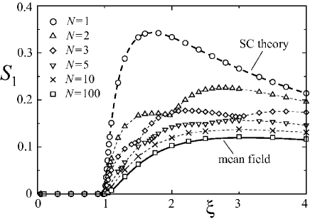
Figure 14: Order parameter $S_{1}=\langle 1/{\tilde{r}}\rangle$ as a function of Manning parameter, $\xi$, for the 2D counterion-cylinder system. Symbols show simulation data for different number of particles as indicated on the graph. The mean-field PB (solid curve) and the strong-coupling (dashed curve) predictions are obtained from Eqs. (52) and (91) respectively, which are valid in 2D as well. The lateral extension parameter here is $\Delta=300$. Thin dashed curves are guides to the eyes.

The order-parameter data in Figure 14, on the other hand, reveal a peculiar set of cusp-like singularities, that are quite pronounced for small number of particles. These points become strictly singular in the limit $\Delta\rightarrow\infty$ and represent the Manning parameters at which individual counterions successively condense (or de-condense). We will demonstrate this point using an analytical approach in Section VIII.3. (A similar singular behavior is also found in 3D for small $N$, but the behavior in 3D appears to be more complex and will not be considered in this paper).

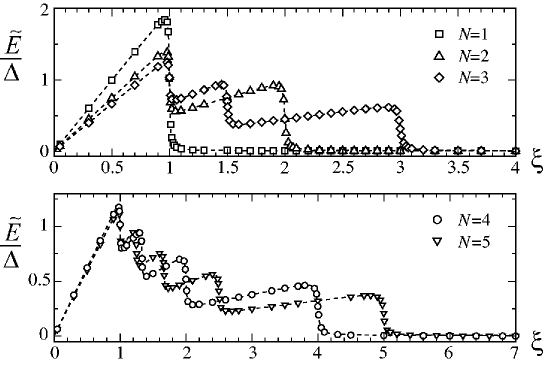
Figure 15: The rescaled (internal) energy of the 2D counterion-cylinder system, $\tilde{E}=E_{N}/(Nk_{\mathrm{B}}T)$, as a function of Manning parameter, $\xi$, for different number of particles as indicated on the graph. Singular regions represent successive condensation (de-condensation) of counterions–see Section VIII.3.1. The lateral extension parameter for these data is $\Delta=300$. The dashed curves are the analytical results given by Eq. (153).

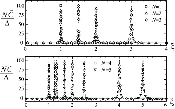
Figure 16: The rescaled excess heat capacity of the 2D system, $\tilde{C}=C_{N}/(Nk_{\mathrm{B}})$, as a function of Manning parameter, $\xi$, for different number of particles, $N$, as indicated on the graph (for clarity, the data are here multiplied by $N$). The peaks represent successive condensation (de-condensation) of counterions–see Section VIII.3.1. For these data $\Delta=300$. The dashed curves are the analytical results given by Eq. (154).

VIII.2 Energy and heat capacity

The singularities at small particle number, $N$, appear also in the internal energy and the heat capacity. In Figures 15 and 16, we plot the rescaled energy, $\tilde{E}=E_{N}/(Nk_{\mathrm{B}}T)$, and excess heat capacity, $\tilde{C}=C_{N}/(Nk_{\mathrm{B}})$, obtained from the simulations using Eqs. (107) and (108) and the 2D Hamiltonian (140), as a function of $\xi$ and for $N=1,2,3,4$ and 5. As seen, the energy shows a sawtooth-like structure for increasing $\xi$ consisting of wide regular regions, in which the energy almost linearly increases, and narrow singular regions, where the energy rapidly drops. Recalling the thermodynamic relation,

$$\xi\frac{\partial\tilde{E}}{\partial\xi}={\tilde{E}}-{\tilde{C}},$$ (145)

it follows that the excess heat capacity vanishes in the regular regions, but develops highly localized peaks in the singular regions, as also seen from the simulation data in Figure 16.

VIII.3 Condensation singularities in 2D: an analytical approach

In what follows, we present an approximate (asymptotic) analysis of the 2D partition, which elucidates the physical mechanism behind the singular behavior in 2D. The rigorous analysis of the 2D problem is still missing and more systematic approximations have been developed recently Burak_unpub .

VIII.3.1 The partition function

Suppose that the Manning parameter is such that $N-m$ counterions are firmly bound to the central cylinder (disk), while $m$ counterions have de-condensed to infinity, where $m=1,\ldots,N$. Using the 2D Hamiltonian (140), the partition function can exactly be written as

$${\mathcal{Z}}_{N}=\int\left[\prod_{i=m+1}^{N}{\mathrm{d}}{{\mathbf{x}}}_{i}\right]\exp\bigg{\{}-\frac{{\mathcal{H}}_{N-m}}{k_{\mathrm{B}}T}\bigg{\}}\times\prod_{l=1}^{m}{\mathcal{Z}}_{N}^{(l)}$$ (146)

in actual units, where ${\mathcal{H}}_{N-m}$ represents interactions among condensed counterions (labeled by $i=m+1,\ldots,N$), and

$${\mathcal{Z}}_{N}^{(l)}=\int{\mathrm{d}}{{\mathbf{x}}}_{l}\,\exp\bigg{\{}-2\xi\ln\bigg{(}\frac{r_{l}}{R}\bigg{)}+\frac{2\xi}{N}\sum_{i=l+1}^{N}\ln\bigg{|}\frac{{{\mathbf{x}}}_{i}-{{\mathbf{x}}}_{l}}{R}\bigg{|}\bigg{\}}$$ (147)

is the contribution from individual de-condensed counterions (labeled by $l=1,\ldots,m$). Assuming that the de-condensed counterions are de-correlated form each other and also from the condensed counterions as they diffuse to infinity for $\Delta\rightarrow\infty$ (i.e. using $|{{\mathbf{x}}}_{i}-{{\mathbf{x}}}_{l}|\simeq r_{l}$), ${\mathcal{Z}}_{N}^{(l)}$ approximately factorizes as

$${\mathcal{Z}}_{N}^{(l)} \simeq 2\pi\!\int\!r_{l}\,{\mathrm{d}}r_{l}\exp\bigg{\{}\!-2\xi\ln\bigg{(}\frac{r_{l}}{R}\bigg{)}+\frac{2\xi}{N}\sum_{i=l+1}^{N}\ln\bigg{(}\frac{r_{l}}{R}\bigg{)}\bigg{\}}$$ (148)

$$= 2\pi R^{2}\,\frac{\exp\big{[}2\big{(}1-\xi l/N\big{)}\Delta\big{]}-1}{2\big{(}1-\xi l/N\big{)}}.$$

In the limit $\Delta\rightarrow\infty$, ${\mathcal{Z}}_{N}^{(l)}$ diverges for Manning parameters

$$\xi\leq\xi_{l}^{s}\equiv\frac{N}{l},$$ (149)

which indicates de-condensation of the $l$-th counterion from the charged cylinder (see Section II.4). Repeating the above argument for various number of de-condensed counterions, one finds a set of singular Manning parameters,

$$\xi_{l}^{s}=\frac{N}{l}\,\,\,\,\,\,\,\,\,\,\,\,\,\,\,\,\,\,\,\,\,{\mathrm{for}}\,\,\,l=1,\ldots,N,$$ (150)

at which individual counterions de-condense from the charged cylinder. These singular points coincide with the values obtained from our simulations based on the full partition function (142) for very large $\Delta$ (see Figures 14-16 and Table 1 for the numerical values).

VIII.3.2 Energy and heat capacity

In general the partition function (146) can exactly be written as

$${\mathcal{Z}}_{N}=\prod_{l=1}^{N}{\mathcal{Z}}_{N}^{(l)},$$ (151)

where ${\mathcal{Z}}_{N}^{(l)}$ is defined in Eq. (147). For $\Delta\gg 1$, the dominant contribution to the internal energy and the heat capacity comes from de-condensed counterions. Thus, in order to derive analytical expressions for energy and heat capacity on the leading-order for large $\Delta$, we shall use Eq. (151) together with the approximate expression (148) for ${\mathcal{Z}}_{N}^{(l)}$. Hence, we obtain the leading-order contribution to the free energy ${\mathcal{F}}_{N}/(k_{\mathrm{B}}T)=-\ln{\mathcal{Z}}_{N}$ as

$${\tilde{\mathcal{F}}}\equiv\frac{{\mathcal{F}}_{N}}{Nk_{\mathrm{B}}T}\simeq-\frac{1}{N}\sum_{l=1}^{N}\ln\frac{e^{2(1-\xi/\xi_{l}^{s})\Delta}-1}{2(1-\xi/\xi_{l}^{s})}$$ (152)

for $\Delta\gg 1$, and thereby the (rescaled) internal energy $\tilde{E}=\xi\partial\tilde{\mathcal{F}}/\partial\xi$ and the rescaled heat capacity $\tilde{C}=-\xi^{2}\partial^{2}\tilde{\mathcal{F}}/\partial\xi^{2}$ are obtained as

$${\tilde{E}}\simeq\sum_{l=1}^{N}\frac{\xi}{N\xi_{l}^{s}}\bigg{(}\frac{2\Delta\,\exp[2(1-\xi/\xi_{l}^{s})\Delta]}{\exp[2(1-\xi/\xi_{l}^{s})\Delta]-1}-\frac{1}{1-\xi/\xi_{l}^{s}}\bigg{)},$$ (153)

$${\tilde{C}}\simeq\sum_{l=1}^{N}\bigg{(}\frac{\xi}{\xi_{l}^{s}}\bigg{)}^{2}\bigg{(}\frac{1}{(1-\xi/\xi_{l}^{s})^{2}}-\frac{\Delta^{2}}{\sinh^{2}[2(1-\xi/\xi_{l}^{s})\Delta]}\bigg{)}.$$ (154)

The above expressions are shown in Figures 15 and 16 for $\Delta=300$ and for various number of particles (dashed curves), which as seen closely reproduce the behavior obtained in the simulations (symbols).

Note that as an individual counterion de-condenses at $\xi_{l}^{s}$, the internal energy suddenly jumps, since the de-condensing counterion gains a large amount of energy due to its logarithmic interaction with the central cylinder. The regular regions (between two successive jumps) in the energy curve are dominated by de-condensed counterions and thus exhibit linear scaling with $\Delta=\ln(D/R)$. The asymptotic form of the energy in these regions for $\Delta\rightarrow\infty$ is obtained from Eq. (153) as

$$\lim_{\Delta\rightarrow\infty}\frac{\tilde{E}}{\Delta}=\frac{l(l+1)}{N^{2}}\xi\,\,\,\,\,\,\,\,\,\,\,\,\,\,{\mathrm{for}}\,\,\,\xi_{l+1}^{s}<\xi<\xi_{l}^{s}.$$ (155)

The singular part of the energy corresponds to a narrow region around each $\xi_{l}^{s}$, which (except for the uppermost singularity) is bounded between a local minimum (slightly above $\xi_{l}^{s}$) and a local maximum (slightly below $\xi_{l}^{s}$). The approximate locations of these extrema are obtained as

$$\frac{\xi_{l}^{\mathrm{min}}}{\xi_{l}^{s}}\simeq 1+\frac{1}{\sqrt{\Delta(l-1)}}\,\,\,\,{\mathrm{and}}\,\,\,\,\frac{\xi_{l}^{\mathrm{max}}}{\xi_{l}^{s}}\simeq 1-\frac{1}{\sqrt{\Delta(l+1)}}$$ (156)

using Eq. (153), and for large $\Delta$. The energy jump, $\delta\tilde{E}_{l}$, upon de-condensation of a counterions at $\xi=\xi_{l}^{s}$ is then given by

$$\delta\tilde{E}_{l}\equiv\tilde{E}(\xi_{l}^{\mathrm{max}})-\tilde{E}(\xi_{l}^{\mathrm{min}})\simeq\frac{2\Delta}{N}.$$ (157)

Note that this value can also be obtained directly from Eq. (155). For $\Delta\rightarrow\infty$ but at fixed and finite $N$, the energy curve tends to a sharp sawtooth-like form as both $\xi_{l}^{\mathrm{min}}$ and $\xi_{l}^{\mathrm{max}}$ tend to $\xi_{l}^{s}$ producing $N$ strictly step-like singular points, at which the limiting energy jump is

$$\lim_{\Delta\rightarrow\infty}\frac{\delta\tilde{E}_{l}}{\Delta}=\frac{2}{N}.$$ (158)

The heat capacity expression (154), on the other hand, exhibits $N$ isolated peaks for $\Delta\gg 1$. The heat capacity at $\xi_{l}$ diverges as $\tilde{C}(\xi=\xi_{l}^{s})\simeq\Delta^{2}/3$ with increasing $\Delta$, giving rise to $N$ limiting algebraic divergencies as

$$\lim_{\Delta\rightarrow\infty}\tilde{C}=\sum_{l=1}^{N}\left(1-\frac{\xi_{l}}{\xi}\right)^{-2}.$$ (159)

VIII.4 Critical point and the continuum limit

The lower-most singularity located at $\xi=\xi^{s}_{N}$ is associated with the de-condensation of the “last” counterion from the charged cylinder. As shown above, this singularity occurs at unity ($\xi^{s}_{N}=1$) when $\Delta\rightarrow\infty$ and is thus independent of the number of counterions. It therefore gives the exact location of the 2D critical point as $\xi_{c}=1$ when the continuum (thermodynamic) limit $N\rightarrow\infty$ is approached, which coincides with the mean-field prediction. Note that in analogy with the method used in Section VI.2, $\xi_{c}$ can also be derived from the asymptotic value of the energy maximum location, Eq. (156), for $l=N$, when $\Delta$ and $N$ both tend to infinity.

Equations (157)-(159) represent the asymptotic results when the system size increases to infinity but the number of particles, $N$, is finite. In the converse limiting case, i.e. when $\Delta$ is large and fixed but $N$ increases to infinity (continuum limit), all singularities smoothen except for the one, which represents the critical point. The limiting energy curve for $N\rightarrow\infty$ may be obtained as follows. First note that the width of the energy jump around each singularity tends to zero as indicated by Eq. (157). Secondly, the spacing between singular points $\xi_{l}^{s}$ (and thus the width of regular regions for $\xi>1$) tends to zero (as $\sim 1/N$) with increasing $N$. Therefore, the energy at a given Manning parameter $\xi$ between two successive singularities, $\xi_{l+1}^{s}<\xi<\xi_{l}^{s}$, is approximately given by $\tilde{E}\simeq\tilde{E}(\xi=\xi_{l}^{s})$, where the right hand side is obtained from Eq. (153) as $\tilde{E}(\xi=\xi_{l}^{s})=\Delta/\xi_{l}^{s}$. This implies that

$$\lim_{N\rightarrow\infty}{\tilde{E}}=\frac{\Delta}{\xi}$$ (160)

for $\xi\geq 1$ and sufficiently large $\Delta$. For small Manning parameter $\xi<1$, there are no singularities and from Eq. (153), we obtain

$$\lim_{N\rightarrow\infty}{\tilde{E}}=2\xi\Delta\times\lim_{N\rightarrow\infty}\sum_{l=1}^{N}\frac{1}{N\xi_{l}^{s}}=\xi\Delta$$ (161)

for large $\Delta$. These limiting results can also be obtained using Eq. (155).

The energy curve in the continuum limit therefore coincides with the universal form obtained within the mean-field theory in Section III.3.2 (see Eq. (82)). The heat capacity in this limit follows from Eq. (110), and exhibits a universal jump at $\xi_{c}=1$ in agreement with Eq. (86).

$N$		$\{\xi^{s}_{N},\ldots,\xi^{s}_{1}\}$
1	1
2	1	2
3	1	3/2	2
4	1	$4/3\simeq 1.33$	2	4
5	1	$5/4=1.25$	$5/3\simeq 1.67$	5/2	5

Table 1: Numerical values of the location of the singularities, Eq. (150), for the 2D counterion-cylinder system for several number of particles (compare Figures 14-16).

VIII.5 The condensed fraction

The preceding results enable us to calculate the limiting condensed fraction of counterions, $\alpha(\xi)$, as well when $\Delta\rightarrow\infty$ and $N\rightarrow\infty$. For a given Manning parameter, $\xi$, and number of particles, $N$, the condensed fraction $\alpha_{N}(\xi)$ is given by the number of singularities located below $\xi$, i.e.

$$\alpha_{N}(\xi)\equiv 1-\frac{l}{N}\,\,\,\,\,\,\,\,\,\,\,\,\,\,\,\,\,{\mathrm{for}}\,\,\,\xi_{l+1}^{s}<\xi<\xi_{l}^{s}.$$ (162)

This fraction is trivially zero for $\xi<\xi_{c}=1$ as $\Delta\rightarrow\infty$. Using Eqs. (150) and (162), we obtain the condition

$$\alpha_{N}(\xi)-\frac{1}{N}<1-\frac{1}{\xi}<\alpha_{N}(\xi),$$ (163)

which in the limit of infinite number of counterions yields

$$\alpha(\xi)\equiv\lim_{N\rightarrow\infty}\alpha_{N}(\xi)=1-\frac{1}{\xi}.$$ (164)

This is nothing but the mean-field or Manning condensed fraction, $\alpha_{\mathrm{M}}=1-1/\xi$ (Section VI.1.2). The finite-ion-number correction to this limiting value follows from Eq. (163) as

$$\alpha_{N}(\xi)-\alpha(\xi)\sim N^{-1}.$$ (165)

IX Conclusion and Discussion

In this paper, we present an extensive numerical analysis of the critical behavior of counterions at a charged cylinder (counterion-condensation transition) in both two and three spatial dimensions. Analytical results for the critical behavior are also derived using the asymptotic theories of mean field (Poisson-Boltzmann) and strong coupling. The counterion-condensation transition (CCT) is regulated by the dimensionless Manning parameter (rescaled inverse temperature), $\xi=q\ell_{\mathrm{B}}\tau$, and occurs at a critical threshold $\xi_{c}$, below which counterions completely unbind (de-condense) to infinity, but above $\xi_{c}$, a finite fraction of counterions binds (or condenses) in the vicinity of the charged cylinder. Since the CCT criticality emerges asymptotically in the limit of infinite system size and infinitely many particles, we have employed Monte-Carlo (MC) simulation of a periodic cylindrical cell model in logarithmic radial coordinates, which gives rise to a powerful (centrifugal) sampling method for extremely large lateral system sizes within reasonable equilibration times. This constitutes the key part of the present numerical investigation, since the critical and universal aspects of the CCT within the cell model can only be captured for large logarithmic system size $\Delta=\ln(D/R)\gg 1$ (with $D$ and $R$ being the outer boundary and the charged cylinder radii respectively).

As main results, we have determined the precise location of the critical Manning parameter, $\xi_{c}$, the scaling universality class of the CCT and the singular behavior of energy and heat capacity on a systematic level and without suppressing inter-particle correlations. As shown both the mean internal energy and the excess heat capacity become singular at the critical point. The excess heat capacity, which vanishes in the de-condensation phase, shows a universal discontinuity (jump) at the critical point indicating that the CCT is a second-order transition, as also suggested in a recent mean-field study Rubinstein01 . In a finite system, these singularities appear in the form of a pronounced peak, the asymptotic behavior of which is used to determine the critical Manning parameter, $\xi_{c}$, in the simulations. On the other hand, the critical exponents associated with the CCT are obtained using a combined finite-ion-number, $N$, and finite-size, $\Delta$, analysis of the order parameters $S_{n}=\langle{\tilde{r}}^{-n}\rangle$ (with $\tilde{r}=r/\mu$ being the radial distance from the cylinder axis in units of the Gouy-Chapman length, $\mu$). These order parameters represent the mean inverse localization length of counterions. For $\xi<\xi_{c}$ and in an infinitely large system, $S_{n}$ vanishes, but takes a finite value above $\xi_{c}$, which exhibits the scaling relation $S_{n}\sim\zeta^{\chi}$, where $\zeta=1-\xi_{c}/\xi$ is the reduced Manning parameter (the reduced temperature) and the exponent $\chi$ is determined as $\chi=2.0\pm 0.4$ within our MC simulations. In finite systems, $S_{n}$ does not vanish at $\xi_{c}$ and displays a power-law decay with increasing size parameters, $\Delta$ and $N$, as $S_{n}(\xi=\xi_{c})=\Delta^{-\gamma}$ (when number of particles, $N$, is fixed) and $S_{n}(\xi=\xi_{c})=N^{-\nu}$ (when lateral extension parameter, $\Delta$, is fixed), where the critical exponents are determined as $\gamma=2.0\pm 0.6$ and $\nu=2/3\pm 0.1$.

The critical exponents are demonstrated to be universal, i.e. independent of the coupling strength, $\Xi$ (varied over several decades $0.1<\Xi<10^{5}$), and agree with the values we obtained from the mean-field PB theory as $\chi_{\mathrm{PB}}=2.0$ and $\gamma_{\mathrm{PB}}=2.0$ (note that the exponent $\nu$ is not defined within mean-field theory). Interestingly, the critical Manning parameter both in 3D and 2D is also found to be universal and given by the mean-field value $\xi_{c}=1$. Therefore, in striking contrast with the typical situation in bulk critical phenomena, where deviations from mean-field theory due to fluctuations grow with decreasing space dimensionality, the CCT criticality is found to be described by the mean-field universality class both in 3D and 2D. Surprisingly, the mean-field theory is found to be exact in 2D in the whole range of Manning parameters (or temperatures) when $N\rightarrow\infty$. In 3D, however, correlation effects in the condensation phase ($\xi>\xi_{c}$) lead to strong deviations from mean-field theory and support the strong-coupling predictions characterized by an excessive accumulation of counterions near the cylinder surface in agreement with previous numerical studies Deserno00 ; Henle04 ; Bratko82 ; Zimm84 ; Rossky85 and experiments Zakha99 . An important result is that the large-distance form of the density profile remains unaffected by these correlations and thereby a universal condensed fraction is obtained when the inflection-point criterion is applied.

To our knowledge, rigorous analytical derivation of the critical Manning parameter or the scaling exponents of the CCT in 3D is not yet available and our simulations provide the first numerical results for the universal and critical features of this transition in the large-system-size limit Naji_CC . In 2D, we have shown that the simulation results can be understood using an approximate analytical theory. The present predictions for order parameters and thermodynamic quantities can be examined in experiments. In particular, the order parameters may be obtained from the distribution of counterions around charged polymers, which has been directly measured using anomalous scattering techniques Das .

In this study, we have made use of an idealized (primitive) cell model Alfrey51 ; Fuoss51 ; Lifson54 in order to bring out the main universal aspects of the CCT. It is interesting to examine possible effects due to more specific factors that exist in realistic situations, namely, the discrete charge pattern of polymers Liu_Muthu02 ; Liao03 ; de-la-Cruz95 ; Manning01 ; Henle04 ; Zimm84 ; Jayaram90 , chain flexibility and finite contour length Ramanathan_Wood82a ; Ramanathan_Wood82b ; Winkler98 ; Liu_Muthu02 ; Liao03 ; de-la-Cruz95 ; Schiess98 ; Nyquist99 ; Muthu04 ; Jayaram90 ; Stevens95 as well as the influence of non-uniform dielectric boundaries Muthu04 on the critical behavior. However, the present results already indicate that short-range effects such as electrostatic correlations do not affect the properties of the system near the critical region ($\xi\sim\xi_{c}$), since most of counterions are de-condensed and the critical behavior is predominately determined by long-range features. Future studies will be useful to address the possible influence of short-range specific effects on the critical behavior Naji_unpub .

In this work, we have not investigated the role of additional salt and co-ions, which lead to screening of electrostatic interactions (see, e.g., Refs. Deserno00 ; Liu_Muthu02 ; Zimm84 ; Rossky85 ). It is known that the Debye screening length, $r_{s}$, plays the role of an upper bound cut-off (similar to the outer boundary $D$ in the cell model): the CCT occurs for vanishing salt concentration, i.e. when $\ln(r_{s}/R)\rightarrow\infty$ Manning69 ; Macgillivray ; Ramanathan ; Shaugh . Thus we can expect similar asymptotic behaviors arise near $\xi_{c}=1$ and within a similar model as used here when the vanishing-salt limit is approached Naji_unpub .

Appendix A Singularities associated with the Onsager instability

The rescaled energy, $\tilde{E}=E_{N}/(Nk_{\mathrm{B}}T)$, and excess heat capacity, $\tilde{C}=C_{N}/(Nk_{\mathrm{B}})$, associated with the Onsager instability can be calculated from Eq. (17). The results coincide with those obtained in Section VIII.3 by choosing $N=1$ (see also Figures 16 and 15). In brief, the approximate location of the energy peak $\xi_{\ast}^{E}$ is obtained as

$$\xi_{\ast}^{E}\simeq 1-\frac{1}{\sqrt{2\Delta}},$$ (166)

for finite large $\Delta$, which shows a different asymptotic convergency (from below) to the critical value $\xi=1$ as compared with the mean-field result, Eq. (112). The heat capacity peak is located above the critical point at

$$\xi_{\ast}^{C}\simeq 1+\frac{5}{\Delta^{2}}.$$ (167)

In the limit $\Delta\rightarrow\infty$, the heat capacity diverges at the critical point from above and below as

$${\tilde{C}}\sim\zeta^{-2}$$ (168)

where $\zeta=1-1/\xi$. The left tail of energy (for $\xi<\xi_{\ast}^{E}$) goes to infinity linearly with $\Delta$ as $\tilde{E}\simeq 2\xi\Delta+\xi/(\xi-1)$, but its right tail shows a power-law divergency as

$${\tilde{E}}\sim\zeta^{-1}.$$ (169)

Note that these behavior are distinctly different from those obtained in the simulations with many particles (Section VI.2) and within the mean-field theory (Section III.3.2).

Appendix B Rescaled PB equation

The Poisson-Boltzmann equation for mean electrostatic potential $\psi_{\mathrm{elec}}$ in actual units reads

$$\nabla^{2}_{\mathbf{x}}\psi_{\mathrm{elec}}=\frac{\sigma({\mathbf{x}})e}{\varepsilon\varepsilon_{0}}-\frac{qe\rho({\mathbf{x}})}{\varepsilon\varepsilon_{0}},$$ (170)

where the density profile of counterions is given by

$$\rho({\mathbf{x}})=\rho_{0}\,\Omega({\mathbf{x}})\,e^{-qe\beta\psi_{\mathrm{elec}}},$$ (171)

with $\rho_{0}$ being a normalization prefactor and $\Omega({\mathbf{x}})$ specifying the volume accessible to counterions (Eq. (20)). The rescaled PB equation (18) is recovered using above equations and the dimensionless parameters as ${\tilde{\mathbf{x}}}={\mathbf{x}}/\mu$, ${\tilde{\sigma}}({\tilde{\mathbf{x}}})=\mu\sigma({\mathbf{x}})/\sigma_{\mathrm{s}}$, ${\tilde{\rho}}({\tilde{\mathbf{x}}})=\rho({\mathbf{x}})/(2\pi\ell_{\mathrm{B}}\sigma_{\mathrm{s}}^{2})$, and also $\psi=qe\psi_{\mathrm{elec}}/(k_{\mathrm{B}}T)$, where $\mu=R/\xi=1/(2\pi q\ell_{\mathrm{B}}\sigma_{\mathrm{s}})$ is the Gouy-Chapman length (Eq. (6)). The prefactor ${\rho_{0}}$ is related to ${\tilde{\kappa}}$ in Eq. (18) through ${\tilde{\kappa}}=\kappa\mu$ where $\kappa^{2}=4\pi q^{2}\ell_{\mathrm{B}}\rho_{0}$. One can show that the density profile in Eq. (171) is also mapped to the rescaled density (23) in the text.

Normalization of the density (to the total number of counterions) in actual units reads $\int{\mathrm{d}}{\mathbf{x}}\,\rho({\mathbf{x}})=N$, and in rescaled units, we have $\int{\mathrm{d}}{\tilde{\mathbf{x}}}\,{\tilde{\rho}}({\tilde{\mathbf{x}}})=2\pi\Xi N$, which is equivalent to Eq. (21) in the text, when Eqs. (11) and (23) are used.

Appendix C Asymptotic results within the PB theory

C.1 Limiting behavior of $\beta$ for large $\Delta$

A general discussion has been given by Fuoss et al. Fuoss51 for the overall behavior of $\beta$ using Eq. (32). Here, we first review some of their results as quoted in the text, and then derive the finite-size scaling relations for $\beta$ near the PB critical point ($\xi_{c}^{\mathrm{PB}}=1$) as used in Section III.3.

C.1.1 Small Manning parameter $\xi<\Lambda_{\mathrm{AF}}$:

The integration constant $\beta$ vanishes at $\xi=\Lambda_{\mathrm{AF}}$ and tends to unity, $\beta\rightarrow 1^{-}$, for small $\xi\rightarrow 0^{+}$, as it can be checked easily from Eq. (32) (we arbitrarily choose $\beta\geq 0$) Fuoss51 . Further inspection shows that in this regime, $\beta\rightarrow(\xi-1)^{-}$ when $\Delta\rightarrow\infty$ Fuoss51 . Hence for $\Delta\gg 1$, one can propose the following form

$$\beta^{2}\simeq(\xi-1)^{2}(1-x),$$ (172)

where $x$ is a small function of $\xi$ and $\Delta$. To determine $x$, we may rearrange the first equation in (32) as

$$\beta\Delta=\frac{1}{2}\ln\frac{1-\beta}{1+\beta}-\frac{1}{2}\ln\frac{(\xi-1)+\beta}{(\xi-1)-\beta}.$$ (173)

and use this together with Eq. (172) to obtain

$$x\simeq\frac{4\xi}{2-\xi}e^{2(\xi-1)\Delta},$$ (174)

which reproduces Eq. (43) in the text.

C.1.2 Large Manning parameter $\xi>\Lambda_{\mathrm{AF}}$:

For large Manning parameter $\xi>\Lambda_{\mathrm{AF}}$, $\beta$, Eq. (32), tends to a finite upper bound $\beta_{\infty}=\pi/\Delta$, when $\xi\rightarrow\infty$ Fuoss51 . Thus for $\Delta\rightarrow\infty$, $\beta$ vanishes for the whole range of Manning parameters $\xi>\Lambda_{\mathrm{AF}}\simeq 1$ as used frequently in the text (see e.g. in Eq. (54)).

C.1.3 Finite-size scaling for $\beta$ close to $\xi_{c}^{\mathrm{PB}}$:

Of particular importance in our analysis is the behavior of $\beta$ close to $\xi_{c}^{\mathrm{PB}}=1$. (Since always $\Lambda_{\mathrm{AF}}\leq 1$, we restrict the discussion only to the regime $\xi\geq\Lambda_{\mathrm{AF}}$). Analysis of Eq. (32) shows that for sufficiently large $\Delta$, we have $\beta\simeq\pi/(2\Delta)$ right at the critical point $\xi_{c}^{\mathrm{PB}}=1$. We may then perform a Taylor expansion around $\xi_{c}^{\mathrm{PB}}$ to obtain the approximate form of $\beta$ for small $\zeta=1-\xi_{c}^{\mathrm{PB}}/\xi$. We find

$$\beta(\zeta,\Delta)=\frac{\pi}{2\Delta}+\frac{2}{\pi}\zeta-\frac{8\Delta}{\pi^{3}}\zeta^{2}+{\mathcal{O}}(\zeta^{3}),$$ (175)

which remains valid for $\zeta\Delta<\pi^{2}/4$. This relation clearly indicates a scale-invariant form for $\beta$ when $\Delta\gg 1$. Comparing this with Eq. (62), we find the approximate form of the scaling function ${\mathcal{B}}(u)$ as

$${\mathcal{B}}(u)\simeq\frac{\pi}{2}+\frac{2}{\pi}u-\frac{8}{\pi^{3}}u^{2},$$ (176)

where $u=\zeta\Delta<\pi^{2}/4$. In particular, we have ${\mathcal{B}}(u)\rightarrow\pi/2$ as $u\rightarrow 0$.

The asymptotic behavior of ${\mathcal{B}}(u)$ for $u\rightarrow\infty$ (or equivalently $\Delta\rightarrow\infty$ for finite $\zeta$) can be obtained using a different series expansion, since in this limit $\beta$ becomes singular at $\xi_{c}^{\mathrm{PB}}=1$ and the above expansion breaks down. This is because $\beta$ is always singular (with an infinite first derivative) at $\Lambda_{\mathrm{AF}}$ which tends to the critical Manning parameter Fuoss51 . We thus perform an expansion around $\xi=\Lambda_{\mathrm{AF}}$, which yields $\beta\simeq\sqrt{3\zeta/\Delta}$. This gives the asymptotic form of the scaling function as

$${\mathcal{B}}(u)\simeq\sqrt{3u}\,\,\,\,\,\,\,\,\,\,\,\,\,u\rightarrow\infty.$$ (177)

C.2 The PB cumulative density profile

The PB cumulative density of counterions, $n_{\mathrm{PB}}(y)$, is defined through Eq. (102). It can be easily shown that $n_{\mathrm{PB}}(y)$ is a monotonically increasing function of $y=\ln(r/R)$, i.e. ${\mathrm{d}}n_{\mathrm{PB}}/{\mathrm{d}}y\geq 0$ Deserno00 . It is therefore bounded by its boundary values $n_{\mathrm{PB}}(0)=0$ and $n_{\mathrm{PB}}(\Delta)=N$ (see Figure 3).

For $\xi>\Lambda_{\mathrm{AF}}$, $n_{\mathrm{PB}}(y)$ has an inflection point the location of which, $y_{\ast}=\ln(r_{\ast}/R)$, follows from equation ${\mathrm{d}}^{2}n_{\mathrm{PB}}/{\mathrm{d}}y^{2}=0$ as $y_{\ast}=\tan^{-1}[(\xi-1)/\beta]/\beta$. It is easy to check (using the results in Appendix C.1) that $y_{\ast}\simeq\Delta/2$ for large $\xi$ and that $y_{\ast}\rightarrow 0$ for $\xi\rightarrow 1$ ($y_{\ast}$ becomes negative for smaller values). For $\xi<\Lambda_{\mathrm{AF}}$, on the other hand, the cumulative density, $n_{\mathrm{PB}}(y)$, vanishes for $y<\Delta$ as $\Delta\rightarrow\infty$, as can be checked by inserting the approximate expression (172) for $\beta$ into Eq. (102).

We note that the main quantities of interest within the PB theory can be expressed solely in terms of the cumulative density profile. This includes the PB potential field $\psi_{\mathrm{PB}}$ and the order parameters $S_{n}^{\mathrm{PB}}$. Using the definitions of these quantities (Section III), we obtain the following relations (which are valid for all $\xi$)

$$\psi_{\mathrm{PB}}(y)=2\xi\bigg{(}y-\frac{1}{N}\int_{0}^{y}\,n_{\mathrm{PB}}(y^{\prime})\,{\mathrm{d}}y^{\prime}\bigg{)}$$ (178)

$$S_{n}^{\mathrm{PB}}=\frac{1}{\xi^{n}}\int_{0}^{\Delta}\,{\mathrm{d}}y\,e^{-ny}\bigg{(}\frac{1}{N}\frac{{\mathrm{d}}n_{\mathrm{PB}}}{{\mathrm{d}}y}\bigg{)}.$$ (179)

C.3 Asymptotic behavior of $S_{n}$ within PB theory

C.3.1 Large Manning parameter $\xi>\Lambda_{\mathrm{AF}}$:

Consider the exact mean-field expression for $S_{n}^{\mathrm{PB}}$, Eq. (52). The integrand in Eq. (52) is the product of an exponentially decaying factor with an inverse-squared sine-function, which has a series of divergencies at $y_{m}=(m\pi-\epsilon)/\beta$ for integer $m$ and $\epsilon\equiv\cot^{-1}[(\xi-1)/\beta]$. For $\Delta\rightarrow\infty$, we know from Appendix C.1 that $\beta\rightarrow 0$ when $\xi>\Lambda_{\mathrm{AF}}\simeq 1$ implying $\epsilon\rightarrow 0$. In this limit, $\epsilon$ may be expanded as

$$\epsilon\simeq\frac{\beta}{\xi-1}-\frac{\beta^{3}}{3(\xi-1)^{3}}+{\mathcal{O}}(\beta^{5}).$$ (180)

The location of singularities, $y_{m}$, tend to infinity with increasing $\Delta$ except for $m=0$ for which we have $y_{0}=-\epsilon/\beta\rightarrow-1/(\xi-1)$ using Eq. (180). The quantity $S_{n}^{\mathrm{PB}}$ in Eq. (52) is therefore dominated by the lower bound of the integral (around $y=0$) due to the exponentially-decaying integrand. To derive the asymptotic form of $S_{n}^{\mathrm{PB}}$ for large $\Delta$, one can expand the integrand either around the lower limit of the integral $y=0$ or around the singular point $y_{0}$. Both procedures lead to the same scaling relation (54) for $S_{n}$ in the strict limit of $\Delta\rightarrow\infty$ when $\xi$ is close to the critical value $\xi_{c}^{\mathrm{PB}}=1$. But only the second procedure leads to a correct result when $\xi$ increases beyond the critical value. This is because for large $\xi$, the singularity at $y_{0}\sim-1/(\xi-1)$ approaches zero rendering the expansion around $y=0$ a poor approximation.

By expanding the integrand around $y=0$ (up to the first order in $y$), we obtain from Eq. (52) that

$$S_{n}^{\mathrm{PB}} \simeq \frac{\beta^{2}}{\xi^{n+1}\sin^{2}\epsilon}\int_{0}^{\Delta}{\mathrm{d}}y\,e^{-(n+2\xi-2)y}$$ (181)

$$\simeq \frac{\beta^{2}+(\xi-1)^{2}}{\xi^{n+1}(n+2\xi-2)}.$$

This relation reproduces Eq. (53) in the text, which, as explained above, is valid for $\xi$ close to $\xi_{c}^{\mathrm{PB}}=1$.

For larger values of $\xi$, we expand the integrand in (52) around $y_{0}=-\epsilon/\beta$, which yields

$$S_{n}^{\mathrm{PB}}\simeq\frac{\beta/\epsilon}{\xi^{n+1}}\left[1-\frac{n\epsilon}{\beta}e^{n\epsilon/\beta}\Gamma(0,\frac{n\epsilon}{\beta})\right],$$ (182)

where $\Gamma(a,b)$ is the incomplete Gamma function. This relation provides a quite good approximation for $S_{n}$ for large $\Delta$ and in the whole range of $\xi>\xi_{c}^{\mathrm{PB}}=1$. In particular, when the limit $\Delta\rightarrow\infty$ is taken, it yields the correct result for $S_{n}(\xi,\Delta\rightarrow\infty)$ (see Eq. (198) below).

C.3.2 Small Manning parameter $\xi<\Lambda_{\mathrm{AF}}$:

For $\xi<\Lambda_{\mathrm{AF}}\simeq 1$, the order parameters, $S_{n}$, vanish as $\Delta\rightarrow\infty$ indicating complete de-condensation of counterions. To demonstrate this, we use Eq. (179), which, for $\Delta\gg 1$, can be written as

$$\xi^{n}S_{n}^{\mathrm{PB}}=\frac{n}{N}\int_{0}^{\Delta}\,{\mathrm{d}}y\,e^{-ny}n_{\mathrm{PB}}(y)+{\mathcal{O}}(e^{-n\Delta}).$$ (183)

Since the cumulative density is bounded by the number of counterions, $N$, and tends to zero at any finite $y$ for $\xi<\Lambda_{\mathrm{AF}}\simeq 1$ (Appendix C.2), we get $S_{n}^{\mathrm{PB}}\rightarrow 0$ in this regime as $\Delta\rightarrow\infty$.

C.4 PB solution in an unbounded system ($\Delta=\infty$)

In the present study, we have assumed that the counterion-cylinder system is bounded laterally ensuring the normalization of density profile, ${\tilde{\rho}}_{\mathrm{PB}}({\tilde{r}})$, to the total number of counterions, $N$, even in the limit $\Delta\rightarrow\infty$. In a strictly unbounded system (with $\Delta=\infty$), the normalization property of density is not preserved, since a finite fraction of counterions escape to infinity. In this case, the PB equation (18) can be solved by relaxing the normalization condition (21). Assuming the boundary conditions at the cylinder surface as $\psi_{\mathrm{PB}}^{\infty}({\tilde{R}})=0$ and ${\tilde{R}}[{\mathrm{d}}\psi_{\mathrm{PB}}^{\infty}({\tilde{r}}={\tilde{R}})/{\mathrm{d}}{\tilde{r}}]=2\xi$, one finds Netz_Joanny

$$\psi_{\mathrm{PB}}^{\infty}({\tilde{r}})=\left\{\begin{array}[]{ll}2\xi\ln\frac{\tilde{r}}{\tilde{R}}&{\,\,\,\xi\leq\xi_{c}^{\mathrm{PB}}=1,}\\ \\ 2\ln\frac{\tilde{r}}{\tilde{R}}+2\ln\left[1+(\xi-1)\ln\frac{\tilde{r}}{\tilde{R}}\right]&{\,\,\,\xi\geq\xi_{c}^{\mathrm{PB}}=1.}\end{array}\right.$$ (187)

Also ${\tilde{\kappa}}^{2}={\tilde{\rho}}_{\mathrm{PB}}^{\infty}({\tilde{R}})=0$ for $\xi\leq\xi_{c}^{\mathrm{PB}}=1$ and ${\tilde{\kappa}}^{2}/2=(\xi-1)^{2}/\xi^{2}$ otherwise. Hence using Eq. (23), we have the density profile in a strictly unbounded system (for $\tilde{R}\leq\tilde{r}\leq\tilde{D}$)

$${\tilde{\rho}}_{\mathrm{PB}}^{\infty}({\tilde{r}})=\left\{\begin{array}[]{ll}0&{\xi\leq 1,}\\ \\ \frac{(\xi-1)^{2}}{\xi^{2}}\left[\frac{\tilde{r}}{\tilde{R}}\right]^{-2}\left[1+(\xi-1)\ln\frac{\tilde{r}}{\tilde{R}}\right]^{-2}&{\xi\geq 1,}\end{array}\right.$$ (191)

which has the same form as given in Eqs. (44) and (46). But now ${\tilde{\rho}}_{\mathrm{PB}}^{\infty}({\tilde{r}})$ is normalized to the condensed fraction of counterions, $\alpha_{\mathrm{M}}$ (Eq. (99)), i.e.

$$\int_{\tilde{R}}^{\infty}{\mathrm{d}}{\tilde{r}}\,\,{\tilde{r}}\,{\tilde{\rho}}_{\mathrm{PB}}^{\infty}({\tilde{r}})=\alpha_{\mathrm{M}}\xi=\left\{\begin{array}[]{ll}0&{\,\,\xi\leq\xi_{c}^{\mathrm{PB}}=1,}\\ \\ \xi-1&{\,\,\xi\geq\xi_{c}^{\mathrm{PB}}=1}\end{array}\right.$$ (195)

(compare with Eq. (41)). The order parameters in the unbounded system, $S_{n}^{{\mathrm{PB}},\infty}$, may be calculated using ${\tilde{\rho}}_{\mathrm{PB}}^{\infty}$. For $\xi>\xi_{c}^{\mathrm{PB}}=1$, we obtain

$$S_{n}^{{\mathrm{PB}},\infty}=\frac{1}{\xi^{n}}\left[1-\frac{n}{\xi-1}e^{n/(\xi-1)}\Gamma(0,\frac{n}{\xi-1})\right].$$ (196)

In the vicinity of the critical point ($\xi\rightarrow 1^{+}$), we get

$$S_{n}^{{\mathrm{PB}},\infty}(\zeta)\sim\frac{\zeta}{n},$$ (197)

which exhibits a different exponent as compared with the quantity $S_{n}^{\mathrm{PB}}(\zeta,\Delta\rightarrow\infty)$ in Eq. (54). This is again due to the difference in normalization factor, which enters in $S_{n}$ through Eq. (50) (note the order in which the integration and the infinite-system limit are taken). In general, the order parameter $S_{n}^{\mathrm{PB}}(\zeta,\Delta\rightarrow\infty)$ is obtained by multiplying $S_{n}^{{\mathrm{PB}},\infty}(\zeta)$ with the condensed fraction $\alpha_{\mathrm{M}}$, as

$$S_{n}^{\mathrm{PB}}(\zeta,\Delta\rightarrow\infty)=\alpha_{\mathrm{M}}S_{n}^{{\mathrm{PB}},\infty}(\zeta).$$ (198)

Appendix D Hamiltonian of a periodic cylindrical cell model (3D)

As stated in Section V.2, the periodic boundary conditions used in the simulations in 3D lead to summation of Coulombic interactions ($v_{\mathrm{3D}}({\mathbf{x}})=1/|{\mathbf{x}}|$) over all periodic images. The resultant summation series are convergent for an electroneutral system and can be mapped to fast-converging series, which can be handled easily in the simulations Lekner ; Sperb . In what follows, we derive the convergent expressions for the configurational Hamiltonian (3).

The main simulation box (of height $L$ and containing $N$ counterions) is replicated infinitely many times in $z$ direction generating a series of $M\rightarrow\infty$ image boxes labeled with $m=-M/2,\ldots,-1,0,1,\ldots,+M/2$ (with $m=0$ being the main box). The Hamiltonian (3) consists of three parts ${\mathcal{H}}_{N}={\mathcal{H}}_{\mathrm{ci}}+{\mathcal{H}}_{\mathrm{int}}+{\mathcal{H}}_{\mathrm{self}}$, namely, counterion-counterion interaction, ${\mathcal{H}}_{\mathrm{ci}}$, counterion-cylinder interaction, ${\mathcal{H}}_{\mathrm{int}}$, and the cylinder self-energy, ${\mathcal{H}}_{\mathrm{self}}$, that will be analyzed separately. (Here we use actual units and in the end, transform the results to the rescaled form.)

D.1 ${\mathcal{H}}_{\mathrm{int}}$ and ${\mathcal{H}}_{\mathrm{self}}$ terms

The counterion-cylinder interaction part per simulation box reads ${\mathcal{H}}_{\mathrm{int}}/(Mk_{\mathrm{B}}T)=\sum_{\alpha=1}^{N}u(r_{\alpha})$, where using $\sigma({\mathbf{x}})=\sigma_{\mathrm{s}}\delta(r-R)$, we have

$$u(r_{\alpha})=-q\ell_{\mathrm{B}}\int v_{\mathrm{3D}}({\mathbf{x}}-{\mathbf{x}}_{\alpha})\sigma({\mathbf{x}}){\mathrm{d}}{\mathbf{x}}=2\xi\ln\bigg{(}\frac{r_{\alpha}}{R}\bigg{)}+c_{0}$$ (199)

with $\alpha$ running only over the counterions within the main box. The constant term is given by

$$c_{0}=-q\ell_{\mathrm{B}}\int v_{\mathrm{3D}}({\mathbf{x}}-{\mathbf{x}}_{0})\sigma({\mathbf{x}})\,{\mathrm{d}}{\mathbf{x}},$$ (200)

where ${\mathbf{x}}_{0}$ belongs to the cylinder surface. $c_{0}$ may be written in terms of the cylinder self-energy,

$$\frac{{\mathcal{H}}_{\mathrm{self}}}{Mk_{\mathrm{B}}T}=\frac{\ell_{\mathrm{B}}}{2}\int\,\sigma({\mathbf{x}})v_{\mathrm{3D}}({\mathbf{x}}-{\mathbf{x}}^{\prime})\sigma({\mathbf{x}}^{\prime})\,{\mathrm{d}}{\mathbf{x}}\,{\mathrm{d}}{\mathbf{x}}^{\prime}.$$ (201)

Using the electroneutrality condition $\tau L=qN$ (per box), one can show that $\beta{\mathcal{H}}_{\mathrm{self}}/(Mk_{\mathrm{B}}T)=-Nc_{0}/2$. Thus, we have

$$\frac{1}{Mk_{\mathrm{B}}T}\bigg{(}{\mathcal{H}}_{\mathrm{int}}+{\mathcal{H}}_{\mathrm{self}}\bigg{)}=2\xi\sum_{\alpha=1}^{N}\ln\bigg{(}\frac{r_{\alpha}}{R}\bigg{)}+C_{0},$$ (202)

where $C_{0}=-\beta{\mathcal{H}}_{\mathrm{self}}/M$ is a constant (see Eq. (4)), which diverges logarithmically with $M$. This can be seen from the asymptotic behavior of the self-energy for large $M$ (or large $ML/R$), i.e.

$$\frac{{\mathcal{H}}_{\mathrm{self}}/(k_{\mathrm{B}}T)}{\tau^{2}\ell_{\mathrm{B}}ML}\! = \!\!\int_{0}^{2\pi}\!\frac{{\mathrm{d}}\theta{\mathrm{d}}\theta^{\prime}}{4\pi^{2}}\!\!\int_{-\frac{ML}{2}}^{\frac{ML}{2}}\!\frac{{\mathrm{d}}z\,{\mathrm{d}}z^{\prime}/(2ML)}{\sqrt{(z-z^{\prime})^{2}+4R^{2}\sin^{2}\frac{\theta-\theta^{\prime}}{2}}}$$ (203)

$$\simeq a_{0}+\ln\bigg{(}\frac{ML}{R}\bigg{)}+{\mathcal{O}}\bigg{(}\frac{R}{ML}\bigg{)}^{2},$$

where $a_{0}\simeq\ln 2-1$. This logarithmic divergency is canceled by a similar divergent term coming from the interaction between counterions (see below).

D.2 ${\mathcal{H}}_{\mathrm{ci}}$ term and the Lekner-Sperb formulae

The contribution from counterionic interactions (per box and for large $M$) can be written as

$$\frac{{\mathcal{H}}_{\mathrm{ci}}}{Mk_{\mathrm{B}}T} = \frac{q^{2}\ell_{\mathrm{B}}}{2M}\sum_{i\neq j}v_{\mathrm{3D}}({\mathbf{x}}_{i}-{\mathbf{x}}_{j})=$$

$$= \frac{q^{2}\ell_{\mathrm{B}}}{2L}\bigg{[}\sum_{\alpha\neq\beta=1}^{N}S_{M}\bigg{(}\frac{{\mathbf{x}}_{\alpha}-{\mathbf{x}}_{\beta}}{L}\bigg{)}+NS_{M}^{0}\bigg{]},$$

where $i$ and $j$ run over all counterions (including periodic images), while $\alpha$ and $\beta$ run over counterions in the main simulation box. We also have $S_{M}^{0}=2\sum_{m=1}^{M/2}m^{-1}$ and

$$S_{M}\bigg{(}\frac{{\mathbf{x}}_{\alpha}-{\mathbf{x}}_{\beta}}{L}\bigg{)}=\sum_{m=-M/2}^{M/2}\bigg{[}\rho_{\alpha\beta}^{2}+(\zeta_{\alpha\beta}+m)^{2}\bigg{]}^{-1/2},$$ (205)

where $\rho_{\alpha\beta}=[(x_{\alpha}-x_{\beta})^{2}+(y_{\alpha}-y_{\beta})^{2}]^{1/2}/L$ and $\zeta_{\alpha\beta}=(z_{\alpha}-z_{\beta})/L$. Note that $S_{M}^{0}$, in particular, represents the interaction between a counterion and its periodic images, which are lined up in $z$ direction. This series diverges and may be written as $S_{M}^{0}=2\ln(M/2)+2{\mathbf{C}}_{e}$ for $M\rightarrow\infty$, where ${\mathbf{C}}_{e}=0.577215\ldots$ is the Euler’s constant. In this limit, $S_{M}$ is also divergent, but it may be split into a convergent and a divergent part as

$$S_{M}=S_{M}^{0}+S_{\mathrm{LS}}(\rho_{\alpha\beta},\zeta_{\alpha\beta})+2(\ln 2-{\mathbf{C}}_{e}),$$ (206)

in which the convergent series $S_{\mathrm{LS}}(\rho_{\alpha\beta},\zeta_{\alpha\beta})$ can be expressed in terms of special functions.

Now inserting the above results for $S_{M}$ and $S_{M}^{0}$ into Eq. (D.2), we have for $M\rightarrow\infty$,

$$\frac{{\mathcal{H}}_{\mathrm{ci}}}{Mk_{\mathrm{B}}T}=\frac{q^{2}\ell_{\mathrm{B}}}{2L}\sum_{\alpha\neq\beta=1}^{N}S_{\mathrm{LS}}(\rho_{\alpha\beta},\zeta_{\alpha\beta})+\xi({\mathbf{C}}_{e}-\ln 2)+\xi N\ln M,$$ (207)

with a logarithmic divergent term (last term) from the one-dimensional periodicity of the system. Using Eqs. (203) and (207), it immediately follows that the divergencies in Eqs. (202) and (207) cancel each other when the electroneutrality condition is assumed. Thus we have the well-defined expression

$$\frac{{\mathcal{H}}_{N}}{Mk_{\mathrm{B}}T}=2\xi\sum_{\alpha=1}^{N}\ln\bigg{(}\frac{r_{\alpha}}{R}\bigg{)}+\frac{q^{2}\ell_{\mathrm{B}}}{2L}\sum_{\alpha\neq\beta=1}^{N}S_{\mathrm{LS}}(\rho_{\alpha\beta},\zeta_{\alpha\beta})+\xi Nh_{0},$$ (208)

where $h_{0}=1+\ln(R/2L)+({\mathbf{C}}_{e}-\ln 2)/N$; equivalently,

$$\frac{{\mathcal{H}}_{N}}{Mk_{\mathrm{B}}T}=2\xi\sum_{\alpha=1}^{N}\ln\bigg{(}\frac{\tilde{r}_{\alpha}}{\tilde{R}}\bigg{)}+\frac{\Xi}{2\tilde{L}}\sum_{\alpha\neq\beta=1}^{N}S_{\mathrm{LS}}(\tilde{\rho}_{\alpha\beta},\tilde{\zeta}_{\alpha\beta})+\xi Nh_{0},$$ (209)

in rescaled units, where $h_{0}=1+\ln(\xi^{2}/2\Xi N)+({\mathbf{C}}_{e}-\ln 2)/N$. The above expression is used to obtain the internal energy and the heat capacity of the system in our simulations (Section V). The term $S_{\mathrm{LS}}(\tilde{\rho}_{\alpha\beta},\tilde{\zeta}_{\alpha\beta})$ may be obtained from Eq. (206) using mathematical identities proposed by Lekner Lekner and Sperb Sperb . It may be written in the form of two formally identical series expansion

$$S_{\mathrm{LS}}=\left\{\begin{array}[]{ll}{\mathrm{I:}}\,-2\ln\tilde{\rho}_{\alpha\beta}+4\sum_{m=1}^{\infty}K_{0}(2\pi m\tilde{\rho}_{\alpha\beta})\cos(2\pi m\tilde{\zeta}_{\alpha\beta}).\\ \\ {\mathrm{II:}}\,\sum_{m=1}^{\infty}{{-1/2}\choose m}\,(\tilde{\rho}_{\alpha\beta})^{2m}\,\bigg{[}Z(2m+1,1+\tilde{\zeta}_{\alpha\beta})\\ \,\,\,\,\,\,\,\,\,\,\,\,\,\,\,-Z(2m+1,1-\tilde{\zeta}_{\alpha\beta})\bigg{]}+(\tilde{\rho}_{\alpha\beta}^{2}+\tilde{\zeta}_{\alpha\beta}^{2})^{-1/2}\\ \,\,\,\,\,\,\,\,\,\,\,\,\,\,-\Psi(1+\tilde{\zeta}_{\alpha\beta})-\Psi(1-\tilde{\zeta}_{\alpha\beta})-c_{\ast}.\end{array}\right.$$ (210)

In the above relations, $K_{0}(x)$ is the modified Bessel function of the second kind, $Z(n,x)=\sum_{k=0}^{\infty}1/(k+x)^{n}$ is the Hurwitz Zeta function, $\Psi(x)$ is the Digamma function, and $c_{\ast}=2\ln 2\simeq 1.386294\ldots$.

The series in Eq. (210) can be evaluated numerically up to the desired accuracy. Note that the first series (Lekner scheme) involves the Bessel function $K_{0}(x)$, which decays exponentially for large $x$ (as $\sim\exp(-x)/\sqrt{x}$) but diverges logarithmically for small $x$. It is therefore rapidly converging when the radial distance between two given particles, $\tilde{\rho}_{\alpha\beta}$, is sufficiently large. We use the following recipe to truncate series I: For $\tilde{\rho}_{\alpha\beta}>3$, we truncate after the third term, for $1/3\leq\tilde{\rho}_{\alpha\beta}\leq 3$, we include $2+[3/\tilde{\rho}_{\alpha\beta}]$ terms in the sum (where $[x]$ refers to the integer part of $x$), and for $1/4\leq\tilde{\rho}_{\alpha\beta}<1/3$, we sum at least 12 terms. This recipe ensures a relative truncation error of about $|e_{r}|\sim 10^{-10}$. For small radial separation $\tilde{\rho}_{\alpha\beta}<1/4$ between two particles, series I becomes inefficient and slow. We thus employ the second series expression (Sperb scheme). This series is rapidly converging for small $\tilde{\rho}_{\alpha\beta}$ provided that $\tilde{\zeta}_{\alpha\beta}$, which enters in the argument of the Hurwitz Zeta function, is sufficiently small, namely for $|\tilde{\zeta}_{\alpha\beta}|\leq 1/2$ Sperb (note that in general we have $|\tilde{\zeta}_{\alpha\beta}|\leq 1$). In fact due to the periodicity of the system, the energy expression (D.2) remains invariant under the transformations $\tilde{\zeta}_{\alpha\beta}\rightarrow 1-\tilde{\zeta}_{\alpha\beta}$ and $\tilde{\zeta}_{\alpha\beta}\rightarrow-\tilde{\zeta}_{\alpha\beta}$, and thus $\tilde{\zeta}_{\alpha\beta}$ can be always restricted to the range $|\tilde{\zeta}_{\alpha\beta}|\leq 1/2$. In this case, we use up to 8 terms in series II. The relative truncation error, $|e_{r}|$, varies for different $\tilde{\zeta}_{\alpha\beta}$, e.g., for $\tilde{\zeta}_{\alpha\beta}\simeq 0.4$ and $\tilde{\rho}_{\alpha\beta}\simeq 0.25$, one has $|e_{r}|\sim 10^{-7}$. The error substantially decreases for smaller $\tilde{\zeta}_{\alpha\beta}$. The above truncation recipes yield accurate estimates for the interaction energies within the statistical error-bars of the simulations.

References

- (1) G.S. Manning, J. Chem. Phys. 51, 924 (1969); 51, 3249 (1969).
- (2) F. Oosawa, Polyelectrolytes (Marcel Dekker, New York, 1971).
- (3) N. Imai, T. Ohnishi, J. Chem. Phys. 30, 1115 (1959); T. Ohnishi, N. Imai, F. Oosawa, J. Phys. Soc. Japan 15, 896 (1960).
- (4) G.S. Manning, Biophys. Chem. 7, 95 (1977).
- (5) G.S. Manning, J. Phys. Chem. 79, 262 (1975); 85, 1506 (1981).
- (6) G.S. Manning, Q. Rev. Biophys. 11, 179 (1978).
- (7) G.S. Manning, Ber. Bunsenges. Phys. Chem. 100, 909 (1996).
- (8) G.S. Manning, Physica A 231, 236 (1996).
- (9) A.D. MacGillivray, J. Chem. Phys. 56, 80 (1972); 56, 83 (1972); 57, 4071 (1972); 57, 4075 (1972).
- (10) G.V. Ramanathan, J. Chem. Phys. 78, 3223 (1983).
- (11) G.V. Ramanathan, C.P. Woodbury, J. Chem. Phys. 77, 4133 (1982); 82, 1482 (1985).
- (12) C.P. Woodbury, G.V. Ramanathan, Macromolecules 15, 82 (1982).
- (13) B.H. Zimm, M. Le Bret, J. Biomol. Struct. Dyn. 1, 461 (1983); M. Le Bret, B.H. Zimm, Biopolymers 23, 287 (1984).
- (14) A. Ikegami, J. Polym. Sci. A 2, 907 (1964).
- (15) R. Zana et al., J. Chim. Phys. Physicochim. Biol. 68, 1258 (1971).
- (16) M. Kowblansky, P. Zema, Macromolecules 14, 166 (1981); 14, 1448 (1981).
- (17) J.W. Klein, B.R. Ware, J. Chem. Phys. 80, 1334 (1984).
- (18) P. Ander, M. Kardan, Macromolecules 17, 2431 (1984).
- (19) L.M. Penafiel, T.A. Litovitz, J. Chem. Phys. 96, 3033 (1992); 97, 559 (1992).
- (20) A. Popov, D.A. Hoagland, J. Polym. Sci. Part B: Polym. Phys. 42, 3616 (2004).
- (21) J.X. Tang et al., Biochemistry 36, 12600 (1997); G.C.L. Wong et al., Phys. Rev. Lett. 91, 018103 (2003).
- (22) V. Bloomfield, Biopolymers 31, 1471 (1991); Curr. Opin. Struct. Biol. 6, 334 (1996).
- (23) R.G. Winkler, M. Gold, P. Reineker, Phys. Rev. Lett. 80, 3731 (1998).
- (24) M. Deserno, C. Holm, S. May, Macromolecules 33, 199 (2000); M. Deserno, Ph.D. thesis, University of Mainz (2000).
- (25) S. Liu, M. Muthukumar, J. Chem. Phys. 116, 9975 (2002); S. Liu, K. Ghosh, M. Muthukumar, J. Chem. Phys. 119, 1813 (2003).
- (26) Q. Liao, A.V. Dobrynin, M. Rubinstein, Macromolecules 36, 3399 (2003).
- (27) M. Fixman, J. Chem. Phys. 70, 4995 (1979)
- (28) D. Stigter, J. Phys. Chem. 82, 1603 (1978); Biophys. J. 69, 380 (1995).
- (29) P. González-Mozuelos, M. Olvera de la Cruz, J. Chem. Phys. 103, 3145 (1995).
- (30) C.A. Tracy, H. Widom, Physica A 244, 402 (1997).
- (31) Y. Levin, M.C. Barbosa, J. Phys. II (France) 7, 37 (1997).
- (32) P.S. Kuhn, Y. Levin, M.C. Barbosa, Macromolecules 31, 8347 (1998).
- (33) H. Schiessel, P. Pincus, Macromolecules 31, 7953 (1998).
- (34) R.M. Nyquist, B.-Y. Ha, A.J. Liu, Macromolecules 32, 3481 (1999).
- (35) J. Ray, G.S. Manning, Macromolecules 32, 4588 (1999).
- (36) H. Qian, J.A. Schellman, J. Phys. Chem. B 104, 11528 (2000).
- (37) G.S. Manning, Macromolecules 34, 4650 (2001).
- (38) A. Deshkovski, S. Obukhov, M. Rubinstein, Phys. Rev. Lett. 86, 2341 (2001).
- (39) P.L. Hansen, R. Podgornik, V.A. Parsegian, Phys. Rev. Lett. 64, 021907 (2001).
- (40) M.L. Henle, C.D. Santangelo, D.M. Patel, P.A. Pincus, Europhys. Lett. 66, 284 (2004).
- (41) M. Muthukumar, J. Chem. Phys. 120, 9343 (2004).
- (42) I. Borukhov, J. Polym. Sci. B: Polym. Phys. 42, 3598 (2004).
- (43) B. O’Shaughnessy, Q. Yang, Phys. Rev. Lett. 94, 048302 (2005).
- (44) A. Naji, R.R. Netz, submitted to Phys. Rev. Lett. (2005); e-print: cond-mat/0504447.
- (45) A.L. Kholodenko, A.L. Beyerlein, Phys. Rev. Lett. 74, 4679 (1995).
- (46) Y. Levin, Physica A 257, 408 (1998).
- (47) Y.Y. Suzuki, J. Phys.: Condens. Matter 16, 2119 (2004).
- (48) R.L. Cleland, Macromolecules 24, 4386 (1991).
- (49) J. Cardy, Scaling and Renormalization in Statistical Physics (Cambridge University Press, Cambridge, 1996).
- (50) T. Alfrey, P.W. Berg, H. Morawetz, J. Polym. Sci. 7, 543 (1951).
- (51) R.M. Fuoss, A. Katchalsky, S. Lifson, Proc. Natl. Acad. Sci. USA 37, 579 (1951).
- (52) R.R. Netz, Eur. Phys. J. E 5, 557 (2001).
- (53) A.G. Moreira, R.R. Netz, Eur. Phys. J. E 8, 33 (2002); Europhys. Lett. 52, 705 (2000).
- (54) A.Yu. Grosberg, T.T. Nguyen, B.I. Shklovskii, Rev. Mod. Phys. 74, 329 (2002); Y. Levin, Rep. Prog. Phys. 65, 1577 (2002).
- (55) A. Naji, R.R. Netz, Eur. Phys. J. E 13, 43 (2004); A. Naji, A. Arnold, C. Holm, R.R. Netz, Europhys. Lett. 67, 130 (2004).
- (56) A. Naji, S. Jungblut, A.G. Moreira, R.R. Netz, Physica A 352, 131 (2005).
- (57) Y. Burak, D. Andelman, H. Orland, Phys. Rev. E 70, 016102 (2004).
- (58) J. DeRouchey, R.R. Netz, J.O. Rädler, Eur. Phys. J. E 16, 17 (2005).
- (59) S. Lifson, A. Katchalsky, J. Polym. Sci. 13, 43 (1954).
- (60) The Onsager divergency may equivalently occur when the lower bound of the integral (cylinder radius) tends to zero Manning69 , since only the ratio is relevant (through ).
- (61) R.R. Netz, J.-F. Joanny, Macromolecules 31, 5123 (1998).
- (62) Note that the density moments for are divergent since for finite , a finite fraction of the counterions is always de-condensed.
- (63) A. Naji, R.R. Netz, C. Seidel, Eur. Phys. J. E 12, 223 (2003)
- (64) D. Bratko, V. Vlachy, Chem. Phys. Lett. 90, 434 (1982).
- (65) M. Le Bret, B.H. Zimm, Biopolymers 23, 271 (1984).
- (66) C.S. Murthy, R.J. Bacquet, P.J. Rossky, J. Phys. Chem. 89, 701 (1985)
- (67) N. Metropolis et al., J. Chem. Phys. 21,1087 (1953).
- (68) J. Lekner, Physica A 176, 485 (1991).
- (69) R. Sperb, Mol. Simul. 20, 179 (1998).
- (70) A. Arnold, C. Holm, Comput. Phys. Commun. 148, 327 (2002).
- (71) H. Flyvberg, H.G. Petersen, J. Chem. Phys. 91, 461 (1989).
- (72) R. Bacquet, P.J. Rossky, J. Phys. Chem. 88, 2660 (1984)
- (73) S.S. Zakharova et al., J. Chem. Phys. 111, 10706 (1999)
- (74) A.W.C. Lau, D.B. Lukatsky, P. Pincus, S.A. Safran, Phys. Rev. E 65, 051502 (2002).
- (75) A.M. Ferrenberg, D.P. Landau, Phys. Rev. B 44, 5081 (1991).
- (76) M.E. Fisher, M.N. Barber, Phys. Rev. Lett. 28, 1516 (1972).
- (77) K. Binder, D.W. Heermann, Monte Carlo Simulation in Statistical Physics: An Introduction, (Springer-Verlag, Berlin, 1988).
- (78) M. Kardar, R. Golestanian, Rev. Mod. Phys. 71, 1233 (1999).
- (79) Y. Burak, H. Orland, preprint (2005).
- (80) R. Das et al., Phys. Rev. Lett. 90, 188103 (2003).
- (81) B. Jayaram et al., Macromolecules 23, 3156 (1990).
- (82) M.J. Stevens, K. Kremer, J. Chem. Phys. 103, 1669 (1995).
- (83) A. Naji, R. R. Netz, unpublished (2005).