Topological kinematic constraints: quantum dislocations and the glide principle.

Abstract

Topological defects play an important role in physics of elastic media and liquid crystals. Their kinematics is determined by constraints of topological origin. An example is the glide motion of dislocations which has been extensively studied by metallurgists. In a recent theoretical study dealing with quantum dualities associated with the quantum melting of solids it was argued that these kinematic constraints play a central role in defining the quantum field theories of relevance to the description of quantum liquid crystalline states of the nematic type. This forms the motivation to analyze more thoroughly the climb constraints underlying the glide motions. In the setting of continuum field theory the climb constraint is equivalent to the condition that the density of constituent particles is vanishing and we derive a mathematical definition of this constraint which has a universal status. This makes possible to study the kinematics of dislocations in arbitrary space-time dimensions and as an example we analyze the restricted climb associated with edge dislocations in 3+1D. Very generally, it can be shown that the climb constraint is equivalent to the condition that dislocations do not communicate with compressional stresses at long distances. However, the formalism makes possible to address the full non-linear theory of relevance to short distance behaviors where violations of the constraint become possible.

I Introduction

Topological defects in crystals topological_defects ; kleman ; kleman1 ; mermin ; klemanbook exhibit a rich variety of kinematic properties Friedel ; Nabarro ; HirthLothe . Defects such as interstitials/vacancies, dislocations, and disclinations Friedel ; Nabarro ; HirthLothe ; Kleinert perturb the ideal perfectly periodic crystal. To date, numerous works extensively studied the dynamics and coarsening of these defects, e.g. Hatano ; CB ; KHEG ; ASV ; RR ; deem . In normal solids, dislocations are present at low concentrations and their peculiar ‘glide motions’ are an important factor in determining the plastic properties of the medium. It has long been recognized that the energy-entropy balance of topological defects is responsible (via deconfinement) for melting transitions polyakov ; Prls ; Onsager ; shock ; burakovsky ; KT ; Mott ; FisherHalperinMorf . In glasses, an extensive configurational entropy of these defects glass (from which ensuing restrictive slow dynamics might follow wolynes ) may be sparked. Investigations of Frank Kasper phases FK1 of defect lines and of related systems FK2 ; FK3 ; FK4 ; FK5 ; FK6 ; FK7 ; FK8 have flourished. In some solids, such as shape memory alloys shape_memory , reducing the appearance of defects is a matter of pertinence. The study of topological defects in liquid crystals LC , compounded by the very crisp imaging techniques of these systems, has evolved into a broad field. Topological defects often display sharp dynamical imprints. Perhaps the best studied such dynamical effect is the glide principle which forms the focus of the current article. Throughout the years, much work has been carried out on the classical glide motion of dislocations. Many of these works entail detailed studies of the Peach-Kohler forces between dislocations and Peierls potentials in systems ranging from classical solids to vortex arrays to liquid crystals, e.g. LS ; LBMNR ; RRPBM ; MR ; SV ; AG ; NTS . Although the discussion of our current publication is aimed towards quantum systems, our formalism may be applied with no change to many of these classical systems to rigorously derive, in the continuum limit, the well known classical glide motion (see Fig.(1)) occurring in the absence of interstitials/vacancies and high order effects. This rigorous result concerning the linear regime of continuum limit elasticity complements older works addressing detailed climb diffusion in various systems, e.g. bruinsma . We further report on new generalized glide equations in the presence of both dislocations and disclinations. As we illustrate in detail here, the basic physical ingredient leading to these generalized glide equations in solids is mass conservation which strictly restrains the dynamics.

Recent years saw the extension of investigations of defect dynamics in classical media to quantum systems ZMN addressing electronic liquid crystal KFE and other phases ZMN ; KFE in which the electronic constituents favor, in a certain parameter regime, the formation of an ideal crystal like stripe pattern which may then be perturbed, through a cascade of transitions, to produce a rich variety of phases. Such stripe patterns are observed in the high temperature superconductors and other oxides tranquada and in quantum Hall systems qhe . Defects naturally alter the local electronic density of states allowing for spatial (and temporal) inhomogeneities of electronic properties zhu . Following the general notion that melting occurs by the condensation of topological defects, e.g. polyakov , we may naturally anticipate that the study of topological defects is pertinent to the understanding of quantum phase transitions between various zero-temperature states. Much unlike classical physics where statics and dynamics are decoupled, in quantum systems, time and space are deeply entangled. As a consequence, we expect the zero point kinematics of defects to be of paramount importance both to the character of the zero-temperature states and to the nature of the phase transitions. Only quite recently, along with Mukhin, two of us ZMN presented a thorough analysis of the problem of topological quantum melting of a solid in 2+1 space-time dimensions. At first sight, this follows the pattern of the famous Nelson-Halperin-Young NH ; Young theory of classical melting in 2D. However, the quantum problem is far richer. Leaning heavily on the formalism developed by Kleinert Kleinert , it was shown in ZMN that the transition from elastic solid to nematic (or ‘hexatic’) liquid crystal is closely related to the vortex (or ‘Abelian Higgs’) duality in 2+1D. The nematic quantum fluid can be viewed as a Bose-condensate of dislocations subjected to a ‘dual’ Higgs mechanism. In this formalism, the rigidity of the elastic medium is parameterized in terms of gauge fields (‘stress photons’). In the quantum fluid, the shear components acquire a Higgs mass due to the presence of the dislocation superfluid. As it turns out, such a substance is at the same time a conventional superfluid, which may now be viewed as an elastic medium which has lost its capacity to sustain shear stress.

The glide principle as known from metallurgy amounts to the observation that dislocations only move easily in the direction of their (vectorial) topological charge. In the nematically ordered state, the Burgers vectors of the dislocations forming the condensate are oriented along the macroscopic director leading to an anisotropic screening of the shear stress ZMN . Here, the dislocations coast freely only in the direction of their director. Accordingly, the elastic propagator can only be fully screened in the direction perpendicular to the director. Even more striking, it turns out ZMN that in the quantum field-theoretic setting the glide principle acquires a meaning which goes well beyond the conventional understanding of this phenomenon. In fact, the main goal of this paper will be to further generalize these notions beyond the linearized continuum limit of ZMN , including a study of theory in higher dimensions and the incorporation of far richer defect configurations.

In many standard texts, e.g.Friedel ; Nabarro ; HirthLothe , the explanation of glide takes little effort. A dislocation corresponds with a row of particles (atoms) ‘coming to an end’ in the middle of a solid. One way to move this entity is to cut the neighboring row at the ‘altitude’ of the dislocation and consequently move over one tail to cure the cut (Fig. 1). The net effect is that the dislocation is displaced. This easy mode of motion is termed ‘glide’. Moving in the orthogonal direction is not as easy. Let us try to move the dislocation ‘upward’. This requires loose particles to make the row of particles longer or shorter (‘interstitials’ or ‘vacancies’) and since loose particles are energetically very costly while they move very slowly (by diffusion) this ‘climb’ motion is strongly hindered. Estimates on ‘climb’ diffusion rates are provided in e.g. bruinsma . Climb is hindered to such an extent in real life situations (e.g. pieces of steel at room temperature) that it may be ignored altogether. The lower dimensional glide motion of dislocations is reminiscent of dynamics in the heavily studied sliding phases slide in which an effective reduction of dimensionality occurs.

Figure 1: An edge dislocation in a two dimensional medium. Here, allowed (matter conserving) cutting and reconnecting of ‘atomic columns’ gives rise to the glide motion of the dislocation line (at the center of figure) in the horizontal direction. By contrast, an emission or absorption of vacancies and interstitials is required for a climb motion (vertical motion of the dislocation in this figure). Thus, an absence of additional material (mass conservation) strictly prohibits the climb within, continuum limit, linear elasticity.

Although this simple pictorial explanation suffices for practical matters in metallurgy, it is immediately obvious that there is more to it. Dislocations are completely specified by their topological charge, the Burgers vector. Expressed in this language, glide is a prescription of the dynamics of defects as dictated by their own topology: dislocations can only move in the direction of their Burgers vector! How can this be?

As we review in section II, this kinematic role of topology arises most naturally in the context of field theoretic description of plasticity. Linear elasticity does not capture interstitial/vacancy defects. The only degrees of freedom which are admitted by continuum limit linear elasticity are phonons (or, in dualized form, the stress photons). Given the absence of interstitials, the secret behind glide is that normal crystals are ‘non-relativistic’- solids cannot displace along the time direction. As the field theory lacks knowledge of the interstitials, this condition translates (as we will illustrate in section IV) directly into the glide constraint for the dislocation matter!

From the glide constraint it immediately follows that gliding dislocations do not occupy volume. Volume is exclusively associated with interstitial matter. Accordingly, dislocations do not communicate with compressional stress and in the dislocation condensate pressure stays massless because of the glide constraint! It better be so, because the dislocation condensate corresponds with a conventional superfluid, and conventional non-relativistic fluids carry sound. Amusingly, glide needs a preferred time direction and in a relativistic medium there is no such thing as a preferred direction. As Kleinert and one of us pointed out KZ , since glide cannot be defined in a truly relativistic medium, dislocations have to couple to compressional stress with the effect that in the relativistic quantum nematic crystal sound also acquires a mass: this incompressible state turns out to be nothing else than the space time of 2+1D general relativity.

The main limitation of ZMN ; KZ is that they focus is exclusively on the special case of dislocation glide in 2+1 dimensions within the realm of the linearized theory. Our main result, presented in section IV, amounts to expressions for new glide-type constraints in arbitrary dimensions. We further investigate what these constraints imply for both dislocations and disclinations via an analogous study of the more fundamental double curl defect densities. In addition, we show in section V how these wisdoms come to an end in the full non-linear theory where dislocations can in principle climb, acting as sources and sinks of interstitials.

This paper is organized as follows: After reviewing the basics of elasticity and introducing some notations in section II, we derive expressions for the dynamical currents for an arbitrarily dimensional medium in section III. In section IV we deduce a general relation describing the glide constraint as it acts on dislocation, disclination, and defect currents according to the linear theory, which is applicable in arbitrary dimensions. This allows us to analyze the particulars of dislocation glide in 3+1D (as well as in arbitrary higher dimensions). In high dimensions, dislocations are no longer particles but instead extended higher dimensional p-branes with p=1 in 3+1D and p=2 in 4+1D. We will show that the glide constraint influences the center of mass motion of the branes while the relative (transversal) motions of these extended manifolds remain unconstrained. This amounts to a precise mathematical description of the ‘restricted climb’ known from metallurgy. We subsequently turn to the disclination and defect currents and presents proofs for deep- but also disappointing traits of these currents: the mass conservation underlying dislocation glide turns into simple conservation laws. Another important property of the constraint is represented in the symmetry of the constrained current. By identifying this constraint as applying only to the unique (rotational symmetry invariant) ‘singlet’ component of the dynamical dislocation current, the relation of the glide constraint to compression is firmly established. In the final section (Section (V)), we lift this to the full non-linear level incorporating the presence of a lattice cut-off and interstitial matter in the field theory formalism.

II Elastic action and defect densities.

Deformations in ideal crystals are parameterized by displacement fields ${\bf u}={\bf R}-{\bf R}_{0}$, where ${\bf R}$ and ${\bf R}_{0}$ refer to the actual position and the position in the ideal crystal of the constituent, respectively. The action of an elastic medium contains strain, kinetic, and external potential components. These are, in general, functionals of the displacements ${\bf u}$ and their derivatives. The kinetic energy density term is simply ${\cal{K}}=\tfrac{1}{2}\rho(\partial_{t}{\bf u})^{2}$. The incorporation of the kinetic energy density ${\cal{K}}$ in the total Lagrangian density leads to the variational equations of motion for the dynamics of ${\bf u}$ in both quantum systems (with bosonic displacements ${\bf u}$) and simple classical ones. Much throughout, we will perform a Wick rotation (wherein the real time $t$ replaced by $-i\tau$) to Euclidean space-time. In the resulting imaginary-time Euclidean action, the Lagrangian density now becomes an “energy” density given by the sum of kinetic and potential parts. The elastic portion of the Lagrangian density follows from the gradient expansion in terms of the displacements. To leading order (‘first order elasticity’), the elastic energy density is $\partial_{i}u^{a}C_{ijab}\partial_{j}u^{b}$ with $C_{ijab}$ the elastic tensor whose general form is dictated by the symmetries of the medium. In the remainder of the article, we will employ Latin indices to refer to spatial components, while Greek indices will be reserved for space-time components. Einstein summation convention will further be assumed for repeated indices. In full generality, the action will further contain higher order derivatives and anharmonic strain couplings:

$$S_{0}=\int{\rm d}\tau{\rm d}{\bf x}~{}{\cal L}_{0}[{\bf u},\partial{\bf u},\ldots,\partial^{m}{\bf u}],$$ (1)

corresponding to the partition function

$$Z=\int{\cal D}{\bf u}~{}e^{-S_{0}[{\bf u},\partial{\bf u},\ldots,\partial^{m}{\bf u}]}.$$ (2)

In the absence of singularities, the action above corresponds with the simple problem of acoustic phonons. However, when defects are present, the theory becomes far richer. In its full non-linear form, elasticity is closely related to Einstein gravityKZ . In the 1980’s, Kleinert Kleinert achieved a considerable progress by his recognition of the underlying gauge field-theoretic structures, employing the mathematical machinery of gauge theory to penetrate deeper into this subject than ever before; much of this is found in his book. This work focused primarily on the ‘plasticity’ of 3D classical media, and only very recently it was extended to the problem of quantum melting in 2+1DZMN .

The key notion introduced by Kleinert is the dualization of the action Eq.(1) into stress variables to recognize subsequently that stress can be expressed in terms of stress gauge fields or ‘stress photons’. Topological defects then take the form of sources for the stress photons. This follows the same pattern as the vortex (or Abelian Higgs) duality where the phase modes of the superfluid are dualized in $U(1)$ gauge fields, mediating the interactions between vortex sources. This analogy is quite close when only dislocations are in the game. The quantum nematics addressed by two of us earlierZMN are dual superconductors in the same sense that the quantum disordered superfluids (Mott-insulators) can be regarded as dual superconductors, the difference being that in the dislocation condensate shear acquires a Higgs mass while in the vortex condensate super-currents acquire the Higgs mass. When disclinations come into play, we need to employ rank two tensorial gauge fields (‘double curl gauge fields’). On this level, the correspondence with gravity become manifestKZ . As this construct is not widely known, we summarize the basic dualization steps in Appendix A.

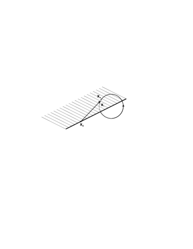
Figure 2: Weingarten theorem: encircling a defect line in a three dimensional medium results in a displacement that depends exclusively on the starting/ending point ${\bf x}_{\pm}$. The discontinuity occurs at the Volterra cut (rastered plane).

There is a famous theorem due to Weingarten Weingarten which states that the singular displacement recorded by encircling a defect line in a three-dimensional elastic medium may always be expressed as a sum of a constant vector and an antisymmetric operator acting on the radial vector ${\bf x}$ (see Fig. 2)

$$\oint_{C}({\rm d}{\bf l}\cdot\nabla){\bf u}={\bf u}({\bf x}_{+})-{\bf u}({\bf x}_{-})={\bf b}_{0}+\hat{\mathscr{A}}({\bf x}-{\bf x}_{0}).$$ (3)

The reference point ${\bf x}_{0}$ can be arbitrary, but when fixed on the defect line it defines the Burgers vector ${\bf b}$ or ‘dislocation charge’ of the defect. The three-dimensional antisymmetric operator $\hat{\mathscr{A}}$ can be represented as the cross product of the radial vector ${\bf x}$ with the pseudo-vector $\Omega$: $\hat{\mathscr{A}}{\bf x}=\Omega\times{\bf x}$. The pseudo-vector $\Omega$ is the Frank vector or the ‘disclination charge’ of the defect. This theorem makes immediately clear that dislocation and disclination charges are related. For instance, a dislocation can be viewed as a bound state of a disclination and an anti-disclination, while the disclination corresponds with a ‘stack’ of an infinite number of dislocations. When addressing linear elasticity, the proper topological current turns out to be a particular combination of dislocation- and disclination currents (the ‘topological defect current’Kleinert ).

Employing the dualization recipe of Appendix A in three classical dimensions, we can straightforwardly derive differential expressions for the dislocation and disclination densities respectively,

$$\alpha_{i}^{a} = \varepsilon_{ijk}\partial_{j}\partial_{k}u^{a},$$ (4)

$$\Theta_{i}^{a} = \tfrac{1}{2}\varepsilon_{ijk}\varepsilon_{abc}\partial_{j}\partial_{k}\partial_{b}u^{c},$$ (5)

where $\varepsilon$ denotes the 3D antisymmetric (Levi-Civita) tensor. For a defect line in a given spatial direction $i$, the charges in Eqs.(4, 5), derived in Appendix A via a dualization procedure, coincide with the Burgers and Frank vectors, respectively. To see this, consider, for instance, the edge dislocation of Fig.(1). Here, in going around the dislocation point there is a net change of the displacement fields. Couched in standard mathematical terms, the Burgers vector signaling the total variation in the displacement field is, as well known,

$${\bf b}=b\hat{e}_{x}=\oint{\bf\nabla}u^{x}\cdot{\bf dl}=\int\int_{{\cal{D}}}{\bf\nabla}\times{\bf\nabla}u^{x}\cdot\bf{dA}.$$ (6)

In Eq.(6), $\hat{e}_{x}$ denotes a unit vector along the horizontal direction and $\bf{dA}$ is a planar area element within a region ${\cal{D}}$ containing the dislocation point. We recognize the argument of the last integrand in Eq.(6) as the dislocation density of Eq.(4)- ${\bf\nabla}\times{\bf\nabla}u^{x}=\alpha^{x}_{j}\hat{e}_{j}$. Similar considerations lead to the identification of Eq.(5) as the angular mismatch (the disclination) density. A nice construct for its visualization is the Volterra cut Kleinert . Needless to say, the derivation of the defect densities via integrals such as that in Eq.(6) is topological; these forms are valid for any crystal regardless of its fundamental constituents (whether they are classical or quantum matter of one particular statistics or another). In what will briefly follow, within the arena of dynamical defects (Section III), we will elevate the densities of Eqs.(4, 5) into the zero (temporal) component of Euclidean space-time defect currents. As a curiosity, an old famous anecdote concerning time like defects is provided in commentBurgerstau .

As stated earlier, dislocations and disclinations are not independent entities: a dislocation may be viewed as a disclination- antidisclination pair while a disclination is an infinite stack of dislocation lines. Thus, the densities of Eqs.(4, 5) harbor redundant information. This redundancy may be removed by fusing the dislocation and disclination densities into a more fundamental (double curl) topological defect density,

$$\eta_{i}^{a} = \tfrac{1}{2}\varepsilon_{ijk}\varepsilon_{abc}\partial_{j}\partial_{b}\left(\partial_{k}u^{c}+\partial_{c}u^{k}\right)=$$ (7)

$$= \Theta_{i}^{a}+\tfrac{1}{2}\partial_{m}\left[\varepsilon_{min}\alpha_{a}^{n}+\varepsilon_{man}\alpha_{i}^{n}-\varepsilon_{ian}\alpha_{m}^{n}\right].$$

Within this publication, most of our studies of these densities will be within the confines of the linearized theory of elasticity. When higher derivatives of the displacement field ${\bf u}$ appear in the action Eq.(1), the defect densities discussed above will fail to capture all of the relevant singularities. The role of higher order corrections will be briefly touched upon in section V.

Depending on the alignment of the charge vector and the three dimensional defect line, dislocations are classified as edge (perpendicular, $i\neq a$) or screw (parallel, $i=a$), while the disclinations may be of the wedge (parallel, $i=a$), sway (perpendicular, $i\neq a$) or twist variants.

III Dynamical dislocation- and disclination currents in arbitrary dimensions.

In this section, we will generalize the gauge theoretical description of defect currents to higher dimensions limiting ourself to the linearized level (first order elasticity).

As a defect drifts through the medium, the defect charge transforms into dynamical defect current. For the particular case of the 2+1-dimensional medium, such issues were addressed for the first time by two of us ZMN . As a first extension, let us now consider how these currents look like in 3+1D. One has now to dualize the full action including the kinetic term. This is a straightforward extension of the 2+1D case,

$$J_{\mu\nu}^{a} = \varepsilon_{\mu\nu\lambda\rho}\partial_{\lambda}\partial_{\rho}u^{a},$$ (8)

$$T_{\mu\nu}^{\alpha\beta} = \varepsilon_{\mu\nu\lambda\kappa}\partial_{\lambda}\partial_{\kappa}\omega^{\alpha\beta},$$ (9)

with the local rotation given by

$$\omega^{\alpha\beta}=\tfrac{1}{2}\varepsilon_{\alpha\beta\rho\sigma}\partial_{\rho}u^{\sigma}.$$ (10)

The currents are now two forms in the ‘lower’ space time labels, actually keeping track of the fact that the defect lines spread out in world sheets (or 2-Branes) in 3+1D space-time. Obviously, by taking one of these labels to correspond with the time direction one immediately recovers the static densities, $J_{\tau i}^{a}=\alpha_{i}^{a}$ and $T_{\tau i}^{\tau a}=\Theta_{i}^{a}$. The currents with two lower spatial indices correspond with the dynamical currents: the lower indices $ij$ refer to a current in the $i$ direction, of a defect line extending into the $j$ direction.

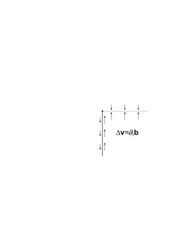
Figure 3: Discontinuity in the velocity field or the ‘velocity dislocation’: such a discontinuity, though physically possible, violates the assumptions of the Weingarten theorem Eq.(3). Depending on the orientation of the Volterra cut with respect to the ‘velocity Burgers vector’ it represents slip of surfaces (parallel, full line) or adding/removing material (perpendicular, dashed line). For simplicity, we use the word ‘slip’ for both motions.

In solids (and other condensed matter systems), the medium cannot displace in the temporal direction $\tau$: $u_{\tau}=0$. Consequently, in the definition of Eq.(8), the‘upper’ Burgers-labels ^a of the dislocation currents $J_{\mu}^{a}$ are purely spatial. Formally, these spatial directions can be regarded as ‘flavor’ degrees of freedom commentBurgerstau . We derive Eq.(9) by employing a generalization the static current of Eq.(5) along with an application of the Weingarten theorem (Eq.(3)). The local rotation operator Eq.(10) used in the definition has also been generalized to deal with the in-equivalence of space and time. When one of the indices $\alpha,\beta$ is temporal, Eq.(10) reduces to the usualKleinert spatial rotation $\omega^{\tau i}=\omega^{i}$. The corresponding disclination current then carries the Frank charge of the defect. What is the physical meaning of the operator Eq.(10) when both indices $\alpha,\beta$ are spatial? Due to the constraint on temporal displacements ($u^{\tau}=0$), the only label that can take the temporal value $\tau$ is $\rho$ and the generalized rotation represents the velocity field

$$\omega^{ab}=\tfrac{1}{2}\varepsilon_{abc}v^{c}.$$ (11)

The corresponding dynamical disclination current $T_{\mu\nu}^{ab}$ records discontinuity, a ‘dislocation’, in the velocity field. Physically, this discontinuity represents slip of two surfaces relative to each other, acting as a ‘defect factory’ in the crystal (Fig. 3). However, the Weingarten theorem, which is the underneath the definitions Eq.(8 - 9), assumes that all the symmetrized strains $u_{\rho,\sigma}=\tfrac{1}{2}(\partial_{\rho}u^{\sigma}+\partial_{\sigma}u^{\rho})$ are smooth everywhere. Choosing one of the indices $\rho$ or $\sigma$ to correspond with time and the other to space, this strain becomes a local rotation,

$$u_{\tau,a}=\tfrac{1}{2}v^{a}=\varepsilon_{abc}\omega^{bc}.$$ (12)

A nonzero value of the disclination current $T_{\mu\nu}^{ab}$ would mean discontinuity in the velocity field, which in turn violates the Weingarten theorem. To avoid confusion between real disclination densities and these surface slips we redefine them as follows,

$$T_{\mu\nu}^{a}=\tfrac{1}{2}\varepsilon_{\mu\nu\lambda\kappa}\varepsilon_{abc}\partial_{\lambda}\partial_{\kappa}\partial_{b}u^{c},$$ (13)

so that only the Frank vector is represented by the upper label (disclination ‘flavor’). When generalized to 3+1D, the dualization procedure summarized in appendix A indicates that the surface slips which we left out will eventually play no role, because they do not couple to stress photons.

Let us now derive the form of the topological currents in arbitrary dimensions. The key lies, once again, in the Weingarten theorem of Eq.(3) which is valid in any dimension. In $D$ dimensional space, the Burgers vector is a $D$-dimensional while the disclination charge is a tensor of rank $D$-2. The rank of the disclination charge may be ascertained from the fact that the antisymmetric tensor $\hat{\mathscr{A}}$ can be written as a contraction of Levi-Civita symbol and another, $D$-2 dimensional antisymmetric tensor: ${\mathscr{A}}_{ij}=\varepsilon_{ijk_{1}k_{2}\ldots k_{D-2}}\Omega_{k_{1}k_{2}\ldots k_{D-2}}$. Thus, two, three and four dimensional disclinations are characterized by a Frank scalar, vector and antisymmetric rank 2 tensor respectively. The $D$+1-dimensional extension of the definitions of the currents Eq.(8,13) are

$$J_{\mu_{1}\ldots\mu_{D-1}}^{a} = \varepsilon_{\mu_{1}\ldots\mu_{D-1}\nu\lambda}\partial_{\nu}\partial_{\lambda}u^{a},$$ (14)

$$T_{\mu_{1}\ldots\mu_{D-1}}^{a_{1}\ldots a_{D-2}} = \tfrac{1}{2}\varepsilon_{\mu_{1}\ldots\mu_{D-1}\nu\lambda}\varepsilon_{a_{1}\ldots a_{D-2}bc}\partial_{\nu}\partial_{\lambda}\partial_{b}u^{c}.$$ (15)

Both of the currents of Eqs.(14,15) are antisymmetric in the lower indices, and represent oriented $p=D-1$-branes. The disclination currents are antisymmetric also in their upper indices where the Frank charge is displayed. We reiterate that within linear elasticity the true (double curl) topological defect density of Eq.(16) removes the redundant information given by the inter-related dislocation and disclination currents. Extending the duality procedure of linearized elasticity (appendix A) to arbitrary dimensions, we easily deduce that the fundamental double curl defect current within a $D$+1 dimensional medium is

$$\eta_{\eta_{1}\eta_{2}\ldots\eta_{D-1}}^{\nu_{1}\nu_{2}\ldots\nu_{D-1}}=$$

$$\tfrac{1}{2}\varepsilon_{\eta_{1}\ldots\eta_{D-1}\kappa\lambda}\varepsilon_{\nu_{1}\ldots\nu_{D-1}\rho\sigma}\partial_{\kappa}\partial_{\rho}(\partial_{\lambda}u^{\sigma}+\partial_{\sigma}u^{\kappa}).$$ (16)

This current is antisymmetric under exchange of any two lower or any two upper indices. This defect current is related to the dislocation and disclination currents Eq.(14 - 15) via

$$\eta_{\eta_{1}\ldots\eta_{D-1}}^{\nu_{1}\ldots\nu_{D-1}}=\sum_{i=1}^{D-1}(-)^{i+1}\delta_{\tau\nu_{i}}T_{\mu_{1}\ldots\mu_{D-1}}^{\nu_{1}\ldots\nu_{i-1}\nu_{i+1}\ldots\nu_{D-1}}+$$

$$+\tfrac{1}{2}\varepsilon_{\mu_{1}\ldots\mu_{D-1}\kappa\lambda}\partial_{\kappa}J_{\nu_{1}\ldots\nu_{D-1}}^{\lambda}+\tfrac{1}{2(D-2)!}\varepsilon_{\mu_{1}\ldots\mu_{D-1}\kappa\lambda}$$

$$\times\varepsilon_{\nu_{1}\ldots\nu_{D-1}\rho\sigma}\varepsilon_{\rho\lambda\xi_{1}\ldots\xi_{D-2}}\partial_{\kappa}J_{\xi_{1}\ldots\xi_{D-2}}^{\sigma}.$$ (17)

To avoid surface slips, one of the upper indices in the definition Eq.(16) must be temporal when addressing the disclination currents $T$. When all the upper indices are spatial, such components record only the derivatives of the dislocation currents of Eq.(14).

IV The electrically charged medium and glide.

Let us now switch gear, to derive mathematical expressions of the glide constraint in terms of the currents introduced above. We consider an electrically charged medium (‘Bosonic Wigner crystal’), both because it is interesting on its own right Wigner ; Ceperley ; EMZMNC , and also because it provides us with a convenient vehicle for the derivation of general expressions for the glide constraint. Later on, we will independently derive these glide constraints by direct mass conservation without resorting to local gauge invariance to implement it. As mass conservation pertains to a scalar quantity, such a conservation law translates into a condition on a linear combination of the topological defect currents which is necessarily invariant under spatial rotations. Conservation laws (equivalent to gauge invariance) may greatly restrict the system dynamics leading to an effective reduction in the dimensionality. We will now illustrate how this indeed transpires in solids: in linear elasticity, mass (‘charge’) conservation allows only a glide motion of a dislocation.

We proceed with the treatment of a charged uniformly charged medium by employing the standard electromagnetic (EM) gauge field formulation. As usual, in Euclidean space, the electrical currents defined in terms of the constituent particles are minimally coupled to the electromagnetic potentials via $ij_{\mu}A_{\mu}$. The spatial current components relate to the velocity of the charged particles, so that every particle with charge $e$ contributes to the current as $(e~{}\partial_{\tau}u^{i})$. For a medium with $n_{e}$ of such particles per unit volume, the corresponding current density will be $j_{i}=(n_{e}e)~{}\partial_{\tau}u^{i}$. The time components describe the coupling between the Coulomb potential $A_{\tau}$ and the charge density $j_{\tau}$. For sufficiently small strains, the density is $[(n_{e}e)~{}(1-\partial_{i}u^{i})]$, subtracting the constant contribution (compensating electrical background). On this linearized level, we should add the following term to the Lagrangian of quantum elasticity to describe the coupling of the EM field to the electrically charged medium,

$${\cal L}_{EM}=i(n_{e}e)~{}[A_{i}\partial_{\tau}u^{i}-A_{\tau}\partial_{i}u^{i}].$$ (18)

The electromagnetic fields further have their own dynamics, described by the Maxwell term ${\cal L}_{Maxwell}=\frac{1}{4}F_{\mu\nu}F_{\mu\nu}$ with field strengths $F_{\mu\nu}=\partial_{\mu}A_{\nu}-\partial_{\nu}A_{\mu}$.

Eq.(18) must be invariant under EM gauge transformations $A_{\mu}\to A_{\mu}+\partial_{\mu}\alpha(x^{\nu})$, with $\alpha(x^{\nu})$ being an arbitrary, non-singular scalar function. The Maxwell term is automatically gauge invariant but the demand of gauge-invariance of the minimal coupling term Eq.(18) implies that the currents are locally conserved. After partial integration,

$$\delta{\cal L}_{EM}=ij_{\mu}\partial_{\mu}\alpha\longrightarrow-i\alpha\partial_{\mu}j_{\mu}.$$ (19)

As $\alpha(x^{\mu})$ is arbitrary, it follows that the current is conserved, $\partial_{\mu}j_{\mu}=0$ – the standard result that gauge invariance implies the conservation of the gauge charge. Let us now see how this works out considering instead the displacement. Performing a gauge transformation on Eq.(18) one finds immediately a gauge non invariant part,

$$\delta{\cal L}_{EM} = i(n_{e}e)~{}[\partial_{i}\alpha\partial_{\tau}u^{i}-\partial_{\tau}\alpha\partial_{i}u^{i}]$$ (20)

$$\longrightarrow i(n_{e}e)\alpha(x^{\mu})~{}[\partial_{\tau}\partial_{i}u^{i}-\partial_{i}\partial_{\tau}u^{i}],$$

and gauge invariance implies that

$$[\partial_{\tau}\partial_{i}u^{i}-\partial_{i}\partial_{\tau}u^{i}]=0$$ (21)

Although this derivation is very simple, this equation is a key result of this paper. Combining it with definition of the dislocation current in arbitrary dimensions Eq.(14) and using the contraction identity,

$$\varepsilon_{\tau a\mu_{1}\ldots\mu_{D-1}}\varepsilon_{\mu_{1}\ldots\mu_{D-1}\nu\lambda}=(D-1)!~{}\left|\begin{array}[]{cc}\delta_{\tau\nu}&\delta_{\tau\lambda}\\ \delta_{a\nu}&\delta_{a\lambda}\end{array}\right|,$$ (24)

it follows that the requirement of conservation of electrical charge has transformed itself into a constraint acting on the dislocation current,

$$\varepsilon_{\tau ai_{1}\ldots i_{D-1}}J_{i_{1}\ldots i_{D-1}}^{a}=0.$$ (25)

This is none other than the glide constraint acting on the dislocation current in arbitrary dimensions!

At first sight this might appear as magic but it is easy to see what is behind this derivation. In order to derive Eq.(18) from Eq.(19) one has to assume that the gradient expansion is well behaved, i.e. the displacements should be finite. This is not the case when interstitials are present, because an interstitial is by definition an object which can dwell away an infinite distance from its lattice position. Hence, in the starting point Eq.(18) it is implicitly assumed that the interstitial density is identical zero. The gauge argument then shows that gauge invariance exclusively communicates with the non-integrability of the displacement fields, Eq.(21). These non-integrabilities are of course nothing else than the topological currents – the glide constraint is a constraint on the dislocation current. If the glide constraint was not satisfied, electrical conservation would be violated locally, i.e. electrical charges would (dis)appear spontaneously, as if the dislocation is capable to create or destroy crystalline matter. In the absence of interstitials this is not possible and, henceforth, dislocations can only glide. The key is, of course, that, by default, dislocation currents are decoupled from compressional stress in the linear non-relativistic theory.

We may, indeed, equivalently derive Eq.(25) without explicitly invoking EM gauge invariance to arrive at Eq.(21). Instead, we may directly rely from the very start on mass conservation- the continuity equation of the mass currents (which, as alluded to above, is equivalent to local gauge invariance), explaintau

$$\partial_{\tau}\rho+\nabla\cdot{\bf j}=0.$$ (26)

To see how this is done directly, we compute the various mass current components $j_{\mu}$. By simple geometrical considerations, within the linear elastic regime, the mass density

$$\rho=\rho_{0}[1-\partial_{i}u^{i}],$$ (27)

with $\rho_{0}$ the uniform background value: the divergence of ${\bf{u}}$ (signaling the local volume increase) yields the negative net mass (‘charge’) density variation at any point. Similarly, the spatial current density

$${\bf j}=\rho_{0}\partial_{\tau}{\bf u}.$$ (28)

Compounding the mass continuity equation of Eq.(26) with the physical identification of the current (Eqs.(27, 28)), we obtain Eq.(21) from which Eq.(25) follows. In section (V), we will return to such a physical interpretation of the glide constraint from this perspective in order to determine corrections to the glide principle which follow from anharmonic terms. We emphasize that the mass conservation law leading to Eq.(21) trivially holds in any medium regardless of the underlying statistics camino of potential quantum systems or their dimension. Furthermore, within the linear elastic regime, such a discussion highlights the validity of Eq.(21) and the ensuing glide equation of Eq.(25) (when interpreted as density matrix averages) in crystals at any temperature in which strict linear order mass conservation condition is imposed on all configurations. Needless to say, as temperature is elevated, a departure occurs from such an imposed linear order condition through the enhanced appearance and diffusion of interstitials and vacancies leading to climb motions. The restriction on the dynamics in this regime is captured by a higher order variant of Eq.(25) (Eq.(55)) which will be derived later on.

Let us now pause to consider what Eq.(25) means physically. In two spatial dimensions, Eq.(25) implies that the dislocation currents have to be symmetric ZMN : $\varepsilon_{ab}J_{a}^{b}=J_{x}^{y}-J_{y}^{x}=0$. Now, consider Fig. (1). Here, the Burgers vector is pointing in the horizontal x-direction implying that $J^{y}_{\mu}=0$, while the glide constraint reduces to $J^{x}_{y}=0$. This current ($J^{x}_{y}$) is, by its very definition, the climb current perpendicular to the Burgers vector.

In three and higher spatial dimensions, the story is less easy, the reason being that the constraint on the motion is less absolute. This is of course known in the classic theory Nabarro ; Kleinert , but the reader might convince him/herself that making use of Eq. (25) the analysis is much helped as compared to the rather pain staking effort based on the ‘intuitive’ arguments. In 3+1D, the constraint of Eq.(25) becomes

$$\epsilon_{\tau abc}J^{a}_{bc}=0.$$ (29)

Let us first consider a screw dislocation. These correspond with dislocation currents of the form $J^{a}_{a\mu}$ (i.e. the static $\mu=\tau$ component corresponds with the orientation of the dislocation loop being parallel to the Burgers vector). It follows immediately that the constraint Eq.(29) is not acting on screw dislocations and, henceforth, screw dislocations can move freely in all directions. Edge dislocations are the other extreme, corresponding with dynamical currents of the form $J^{a}_{b\mu}$ where $a$ and $b$ are orthogonal. The condition $\mu=a$ corresponds with glide: an edge dislocation with its loop oriented in a direction ($b$) perpendicular to the Burgers vector ($a$) can still move freely in the direction of the Burgers vector ($a$). The displacement of a dislocation along the line is not a topological object and the current with two identical lower indices ($\mu=b$) vanishes. The glide constraint only strikes when all three labels are different. Let us consider a dislocation line extending in $z$ direction with Burgers vector in the $x$ direction (see Fig. 4). The only nonzero components of the current are $J_{z\mu}^{x}$ and the glide constraint becomes $J^{x}_{zy}=0$. This automatically forbids any motion in the $y$ direction, that is perpendicular both to the dislocation line and its Burgers vector. The constraint is ‘leaky’ due to the extended nature of the defect. The material needed for the climb of one segment of the dislocation can be supplied by an adjacent segment. The glide constraint has therefore only a real meaning through its integral form,

$$0=\int dV\varepsilon_{\tau abc}J_{ab}^{c}.$$ (30)

As illustrated in Fig. 4, only the dislocation’s ‘center of mass’ is prohibited to move in the climb direction. Local segments of the line may still move at expense of their neighbors, effectively transporting matter along the defect line. The ‘leaky’, locally defined, constraint of Eq.(30) corresponds with the intuitive idea of ‘restricted climb’ found in the elasticity literature.

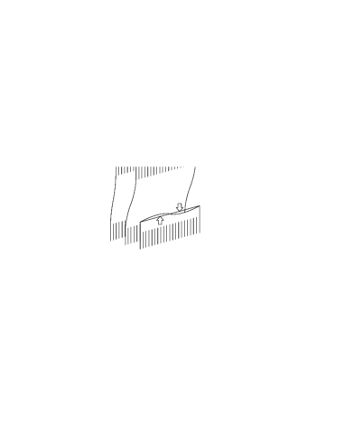
Figure 4: Restricted climb in the 3+1D medium: although the dislocation line cannot displace as a whole in the direction perpendicular to both itself and its Burgers vector (climb direction), local segments may climb at the expense of their neighbors’ height.

Having a mathematical definition of the glide constraint at our fingertips enables us to address its incarnations in even higher dimensional systems where direct visualization is of little use. Notwithstanding that such crystals are, of course, not to be found in standard condensed matter, higher dimensional glide constraints might have implications for ‘emergence theories’ of fundamental phenomena resting on elasticity theory KZ ; KleinertBrJP . Let us for example look how the constraint Eq.(25) acts in a 4+1D crystal. A dislocation is now a 2-brane, say, a plane extending in $y$ and $z$ directions. When its Burgers vector lies in this plane, this brane is analogous to a screw dislocation in the sense that its motions are not affected by the glide constraint. The other extreme is the ‘edge dislocation brane’ with a Burgers vector perpendicular to the brane, say in the $x$ direction. In this case the nontrivial currents correspond with $J_{yz\mu}^{x}$. As noted earlier for three-dimensional defects, topological currents do not record any motion taking place within the defect-brane but only in directions perpendicular to it. The bottom line is that besides the static current (density) $J_{yz\tau}^{x}$, the topological dynamical currents are $J_{yzx}^{x}$ and $J_{yzw}^{x}$, representing dislocation glide and climb respectively. The glide constraint Eq. (25) forbids the latter ‘in integral form’, allowing climb of a certain brane element only at the expense of the brane volume taken by a neighboring element.

IV.1 The glide constraint and motions of general defects.

Up to this point we focused on dislocations, the traditional scenery for glide motions. However, as alluded to in section II, dislocation and disclination currents are not independent. The truly fundamental topological currents are the (double curl) defect currents of Eq.(16). A natural question to ask is what the form of the glide constraint is on these fundamental entities. This task is made easy by Eq.(21). In what follows, we will derive new generalized glide equations for a medium in which both dislocations and disclinations are present.

Let us first consider the most trivial case, the 2+1D crystal. Excluding surface slips, Eq.(17) becomes

$$\eta_{\mu}^{\nu}=\delta_{\nu\tau}T_{\mu}-\tfrac{1}{2}\partial_{\lambda}\left[\varepsilon_{\lambda\mu a}J_{\nu}^{a}+\varepsilon_{\lambda\nu a}J_{\mu}^{a}-\varepsilon_{\mu\nu a}J_{\lambda}^{a}\right].$$ (31)

In two spatial dimensions, we immediately note from Eq.(31) that the glide constraint implies that $\eta_{i}^{i}=0$.

The extension to arbitrary dimensions is straightforward. We start with the definition Eq.(16) and then employ the Levi-Civita contraction identity to obtain

$$\varepsilon_{\mu a_{1}\ldots a_{D-1}\rho\lambda}\varepsilon_{\tau a_{1}\ldots a_{D-1}bc}=(D-1)!\left|\begin{array}[]{c c c}\delta_{\mu\tau}&\delta_{\mu b}&\delta_{\mu c}\\ \delta_{\rho\tau}&\delta_{\rho b}&\delta_{\rho c}\\ \delta_{\lambda\tau}&\delta_{\lambda b}&\delta_{\lambda c}\end{array}\right|.$$ (35)

The terms containing $u^{\tau}$ vanish. The no-slip condition ($\partial_{\mu}\partial_{\nu}v^{a}=\partial_{\nu}\partial_{\mu}v^{a}$) needs to be imposed supplanted by the glide constraint in its strain form of Eq.(20). The outcome is that the scalar spherical tensor component of the general defect current tensor of Eq. (17) vanishes

$$\eta_{a_{1}a_{2}\ldots a_{D-1}}^{a_{1}a_{2}\ldots a_{D-1}}=0.$$ (36)

We next investigate what the glide constraint implies for disclinations. The constraint of Eq.(36) does not shed much light on this issue. Linear elasticity directly addresses dislocations: as we already argued, one of the upper indices in the defect current of Eq.(16) needs to be temporal in order to record disclination currents. On the other hand, it is clear that disclinations somehow do know about glide because they can be viewed as an infinite stack of dislocations. As an example, consider a wedge disclination: the material added by the Volterra cut is proportional to the Frank charge and this should not change over time. It turns out that the matter conservation associated with a general defect distribution is related to the Volterra cutting procedure. After the cut has been applied, no additional material should be introduced, which is the same as the requirement that all symmetrized strains and derivatives thereof are smooth everywhere, including the locus of the Volterra cut. This condition is hard wired into the proof of the generalized Weingarten theorem Eq.(3). As we will now show, the ramification of this principle for disclinations is a conservation law.

To make headway, it is convenient to first consider Euclidean Lorentz-invariant $D+1$ space time. The non-relativistic case will turn out to be a special case which directly follows from imposing the condition of the absence of time like displacements ($u^{\tau}=0$). What follows rests heavily on elastic analogs of identities in differential geometry which are discussed in detail in the last part of Kleinert’s bookKleinert . First, we introduce the tensor

$$R_{\mu\nu,\rho\sigma}=(\partial_{\mu}\partial_{\nu}-\partial_{\nu}\partial_{\mu})\partial_{\rho}u^{\sigma}$$ (37)

representing the Riemann-Christoffel curvature tensor in the geometrical formulation of the theory of elasticity (the $u$’s are crystal displacements). The smoothness assumptions underlying the Weingarten theorem may be expressed as,

$$0 = (\partial_{\mu}\partial_{\nu}-\partial_{\nu}\partial_{\mu})(\partial_{\rho}u^{\sigma}+\partial_{\sigma}u^{\rho}),$$ (38)

$$0 = (\partial_{\mu}\partial_{\nu}-\partial_{\nu}\partial_{\mu})\partial_{\lambda}(\partial_{\rho}u^{\sigma}+\partial_{\sigma}u^{\rho}),$$ (39)

which in turn imply smoothness of the displacement second derivative

$$0=(\partial_{\mu}\partial_{\nu}-\partial_{\nu}\partial_{\mu})\partial_{\lambda}\partial_{\rho}u^{\sigma}.$$ (40)

Cycling through the indices $\mu$, $\nu$, and $\lambda$ of the smoothness equation Eq.(40), we obtain the Bianchi identity for the displacement fields,

$$\partial_{\mu}R_{\nu\lambda,\rho\sigma}+\partial_{\nu}R_{\lambda\mu,\rho\sigma}+\partial_{\lambda}R_{\mu\nu,\rho\sigma}=0.$$ (41)

Starting from the other end, let us analyze a candidate for a disclination conservation law, corresponding with $\partial_{\mu}T_{\mu\nu_{1}\nu_{2}\ldots\nu_{D-2}}^{\phantom{\mu}\alpha_{1}\alpha_{2}\ldots\alpha_{D-1}}$. This can be expressed in terms of the Riemann tensor where ${\alpha}$ refers to a string of indices labeled by ${\alpha}$,

$$\partial_{\mu}T_{\mu\{\nu\}}^{\phantom{\mu}\{\alpha\}} = \tfrac{1}{2}\varepsilon_{\mu\{\nu\}\kappa\lambda}\varepsilon_{\{\alpha\}\rho\sigma}\partial_{\mu}\partial_{\kappa}\partial_{\lambda}\partial_{\rho}u^{\sigma}$$ (42)

$$= \tfrac{1}{2}\varepsilon_{\mu\{\nu\}\kappa\lambda}\varepsilon_{\{\alpha\}\rho\sigma}\partial_{\mu}(\partial_{\kappa}\partial_{\lambda}-\partial_{\lambda}\partial_{\kappa}+\partial_{\lambda}\partial_{\kappa})\partial_{\rho}u^{\sigma}$$

$$= \tfrac{1}{2}\varepsilon_{\mu\{\nu\}\kappa\lambda}\varepsilon_{\{\alpha\}\rho\sigma}\partial_{\mu}R_{\kappa\lambda,\rho\sigma}-\partial_{\mu}T_{\mu\{\nu\}}^{\phantom{\mu}\{\alpha\}}.$$

The first term is zero as a consequence of the contraction of the Bianchi identity Eq.(41) and the Levi-Civita symbol $\varepsilon_{\mu\{\nu\}\kappa\lambda}$. This implies that relativistic disclination currents are conserved. The non-relativistic case is just a special case: the vanishing of time like displacements means that all upper labels are space-like ($\alpha\rightarrow a$) and it follows,

$$\partial_{\mu}T_{\mu\nu_{1}\nu_{2}\ldots\nu_{D-2}}^{\phantom{\mu}a_{1}a_{2}\ldots a_{D-2}}=0.$$ (43)

In the 2+1D medium, only wedge dislocations exist and the message of the conservation law Eq.(43) is clear: the Frank charge- the angle of an inserted wedge in the Volterra construction- behaves as a trivially conserved scalar component of a tensor. In higher dimensions, the disclination current similarly behaves as a conserved tensorial current. The defect density has information regarding both dislocations and disclinations. The disclination conservation law has separate ramifications for the defect density. The fundamental condition Eq.(40) can be directly rewritten into a conservation law for the defect density of a similar form as for the disclinations,

$$\partial_{\mu}\eta_{\mu\nu_{1}\ldots\nu_{D-2}}^{\alpha_{1}\alpha_{2}\ldots\alpha_{D-1}}=0.$$ (44)

This is not surprising as defect currents are proportional to to disclination currents.

This completes the picture: the conservation of matter mandates that the ‘proper’ disclinations currents are also conserved. However, the ‘handicapped’ dislocation currents are not conserved a-priori (disclinations form their sources) but they have to pay the price that they can only glide.

IV.2 Symmetry properties of the constraint

The static dislocations and disclinations of higher dimensional media are geometrically complex entities such as lines, sheets or $d$-branes with Burgers vectors and Frank tensors attached. When in motion, these branes sweep the additional time dimension. For instance, defects in two space dimensions are point-like particles turning into world-lines in space-time, in three space dimensions they form loops spreading out in strings etc. Nevertheless, regardless of the embedding dimensionality, all of these ‘branes’ share an universal property: there is a unique direction perpendicular to the brane. This direction can be related to the dynamical defect currents by contracting it with the $D-1$ dimensional antisymmetric tensor having one index set equal to time,

$$\tfrac{1}{(D-1)!}\varepsilon_{\tau ib_{1}b_{2}\ldots b_{D-1}}J_{b_{1}b_{2}\ldots b_{D-1}}^{a} =$$

$$\partial_{i}\partial_{\tau}u^{a}-\partial_{\tau}\partial_{i}u^{a} = U_{i}^{a},$$ (45)

isolating the perpendicular direction $i$. Instead of the dislocation current $J$, we could have used here also the disclination current $T$, but our interest in this subsection will be in the former. The comparison of the tensor Eq.(45) with the glide constraint Eq.(20) illustrates that the glide condition turns into a constraint on the trace $U_{i}^{i}=0$. For rank 2 tensors, the trace is the only invariant tensorial component of the $D$-dimensional orthogonal group ($O(D)$), corresponding with all rotations and the inversion in the $D$-dimensional medium. It follows that the constrained current is the only ‘singlet’ (scalar) under the point group symmetries of the crystal (point group symmetries constitute a subgroup of $O(D)$). The conjugate degree of freedom must have the same symmetry and this can only be compression, the only physical entity being a singlet under $O(D)$. We have identified the fundamental reason that glide implies the decoupling of dislocations and compressional stressZMN .

Apart from rotations, the glide constraint is also invariant under Galilean space-time translations. Needless to say, the constraint does not obey Euclidean Lorentz (space-time) invariance as the time direction has a special status both in Eq.(20) and Eq.(25). The origin of this lies, of course, in the definition of the crystalline displacement ${\bf u}$ and its role in the minimal coupling Eq.(18). The displacements are defined under the assumption that every crystalline site has an equilibrium position which implicitly wires in that their world lines extend exclusively in the temporal direction. The crystal defect currents (Eq.(36)) and the disclination conservation law of Eq.(43) are invariant under Galilean transformations while they do not respect invariance under Lorentz boosts.

V The Glide constraint, the lattice cut-off and anharmonicity

Contrary to our rigorous (‘glide only’) result concerning the linear regime of continuum elasticity, in real crystals dislocations do climb (albeit at small rates). As discussed earlier by two of usZMN , interstitial matter will be exchanged when dislocations collide and this process releases climb motions. In what follows, we will rederive the glide constraint, yet now do so within a fully general framework which will enable us to address the implications of both (higher order) non-linear elasticity and the presence of a lattice cut-off. Higher order corrections to linear elasticity modify the original glide constraints of Eq.(25) giving rise dislocation climb. We will leave the detailed analysis of the non-linear problem to a later publication anharmonic . In what follows, we outline how the full non-linear theory (including finite lattice size effects) captures higher order effects such as climb.

To achieve this aim, we return to the mass continuity equation invoked earlier (in unison with Eqs.(27, 28)) yet now, by examining contributions of higher order derivatives of the displacement field, we exercise far greater care in examining its ramifications. The continuity equation of Eq.(26) implicitly assumes that the density and current fields are functionals of local Eulerian (distorted lattice) coordinates. On the other hand, the displacement, stress, and other elastic fields are functionals of substantial coordinates (i.e. the coordinates defined relative to the undistorted lattice coordinates)- the Lagrangian coordinate frame. As was briefly done earlier (Eqs.(27, 28)), we express the local density and currents of Eq.(26) in terms of volume and velocities as $\rho=\frac{\rho_{0}}{V}$ and ${\bf j}=\frac{\bf\rho_{0}v}{V}$, with $\rho_{0}$ the mass of the ideal uniform medium in a unit volume in the undistorted original medium (i.e. the ideal background mass density). Following a distortion, a unit volume element of the original medium now occupies a region of volume $V$. With these relations in tow, Eq.(26) reads

$$\partial_{\tau}V+({\bf v}\cdot\nabla)V\equiv D_{\tau}V=V(\nabla\cdot{\bf v}).$$ (46)

This equation can be interpreted as a law governing the change of volume of the elastic medium: the change in volume (the derivative on the left hand side) is exclusively dictated by the motion of the boundaries- the gradient on the right hand side corresponds with a surface integral of the velocity field. This is just a reformulation of the same basic constraint: the conservation of mass (or electrical charge). Throughout this paper, mass conservation was the primary ingredient leading to the glide constraint. To invoke the mass continuity equation in the form of Eq.(46), let us express the actual atomic coordinates $R^{j}$ in terms of the Eulerian coordinates (henceforth denoted by $r^{i}$) by employing the identity,

$$(\frac{\partial R^{j}}{\partial r^{i}})_{\tau}=(\delta_{ij}+\sum_{m=1}^{\infty}\frac{a^{m-1}}{m!}\partial_{j}^{m}u^{i})^{-1},$$ (47)

where $a$ is a (lattice) cut-off scale. Simplifying, we find that Eq. (46) may be recast as

$$\partial_{\tau}V=V~{}(\frac{\partial R^{j}}{\partial r^{i}})_{\tau}\partial_{i}\partial_{\tau}u^{j}.$$ (48)

This is an exact expression (entailing corrections to all order in gradients of ${\bf u}$) detailing the glide constraint. Retaining the leading order contributions and employing $V=1+\partial_{i}u^{i}$, we recover the ‘familiar’ linearized glide constraint of Eq.(20). The exact glide constraint Eq.(48) can also be derived using the coupling to electromagnetism as generating functional as used in section IV.

How may we generalize this analysis so that it deals with the non-linearities up to all orders? A key is provided by Eq.(18). Due to changes in the volume of the medium arbitrarily large lattice deformations translate into current densities $j_{\mu}$. In addition, we should use substantial- instead of local coordinates such that the spatial arguments of the EM fields and strains no longer coincide. A crystalline constituent that was originally at position ${\bf R}$ feels the EM field at point ${\bf R}+{\bf u}$. Hence, the full non-linear generalization of Eq. (18) is

$${\cal L}_{EM}=\frac{(n_{e}e)}{V({\bf R})}[\partial_{\tau}u^{i}({\bf R})A_{i}({\bf R}+{\bf u})+A_{\tau}({\bf R}+{\bf u})].$$ (49)

Using the procedure of Section IV, the exact glide constraint is straightforwardly derived from this expression.

What can we learn from this exact form of the glide constraint? Let us specialize to the simple 2+1D medium. Assuming a vanishing lattice constant $a$, the volume of an elementary cell is simply given as $V=\det(\delta_{ij}+\partial_{i}u^{j})$. Inserting this in the exact glide expression Eq.(48) we find that it simplifies,

$$0=\varepsilon_{ab}J_{i}^{b}(\delta_{ia}+\partial_{i}u^{a}).$$ (50)

The displacement derivative $\partial_{i}u^{a}$ includes both regular and singular components. When $\partial_{i}u^{a}$ is small compared to unity, the linearized glide constraint of Eq.(25) is recovered.

Let us now analyze the conditions required for a dislocation in climbing motion to satisfy the generalized constraint of Eq.(50). As before, we set the Burgers vector of a dislocation to ${\bf b}=b{\bf e}_{x}$ implying $J_{\mu}^{y}=0$. A climbing dislocation then moves in the $y$ direction resulting in the dynamical current ($\overline{x}_{i}$ is the position of the dislocation)

$$J_{y}^{x}=b~{}\partial_{\tau}{\overline{y}}~{}\delta[x_{i}-\overline{x}_{i}(\tau)].$$ (51)

Assuming that the dislocation does not glide simultaneously, the current Eq.(51) is the only nonzero dynamical dislocation current. The exact glide constraint is then satisfied, if and only if

$$0=1+\partial_{y}u^{y}\bigg{|}_{\overline{x}_{i}}.$$ (52)

Clearly, so long as we keep the displacements small compared than the lattice size (effectively prohibiting interstitials and vacancies), the condition of Eq.(52) is impossible to satisfy and climb motion is strictly forbidden. However, as soon as particles are allowed to leave their initial positions in the crystal (interstitial density develops), $\partial_{y}u^{y}$ becomes finite and climb motion is liberated!

More precisely, the right hand side of the condition Eq.(52) represents the derivative of Euler to Lagrangian coordinates $\frac{\partial y}{\partial Y}$ and if vanishing, it means that two neighboring sites of the original crystal are, upon deformation, occupying the same place. This is none other than an interstitial ‘event’. We can thus interpret the 2+1-dimensional exact glide constraint of Eq.(50) as formally proving the old metallurgical maxim that “climb motion is permitted if and only if interstitials/vacancies are present”. This climb will have the effect that the interstitial is absorbed by the dislocation.

We reach the conclusion that higher orders in the displacements (non-linearities, anharmonicities) have the effect of restoring the physics of interstitials. Another natural question to ask regarding the continuum limit is whether there may be a hidden dependence on the lattice cut-off $a$. To investigate this issue, let us see what happens to Eq.(48) when we only keep terms which are harmonic in the displacements, while imposing no conditions on the number of derivatives. These have to do with the volume of the unit cell. Let us specialize to a simple hypercubic lattice with sides defined by the vectors ($i=1,\ldots,D$),

$$u^{j}(R_{i}+a_{i})-u^{j}(R_{i})=\delta_{ij}+\sum_{m=1}^{\infty}\frac{a^{m-1}}{m!}\partial_{i}^{m}u^{j}.$$ (53)

The corresponding volume is a determinant of the matrix Eq.(53) and in the harmonic approximation only the diagonal elements remain,

$$V=1+\sum_{i,j=1}^{D}\sum_{m=1}^{\infty}\frac{a^{m-1}}{m!}\partial_{i}^{m}u^{j}.$$ (54)

Using this expression for the volume, the exact equation of constraint (Eq. (48)) reads

$$\varepsilon_{\tau ai_{1}...i_{D-1}}J^{a}_{i_{1}...i_{D-1}}$$

$$=-(D-1)!\sum_{i=1}^{D}\partial_{\tau}\frac{e^{a\partial_{i}}-a\partial_{i}-1}{a\partial_{i}}\partial_{i}u^{i}.$$ (55)

The remarkable fact is that it is possible to collect all higher order derivatives in a simple exponent.

Eq.(55) amounts to a double check on the non-singular nature of the continuum limit. It corresponds with a resummation to all orders and if there would be a non-perturbative surprise it should show up in this equation. One sees immediately that this is not the case: in the long wavelength limit ($q\to 0$), the spatial derivatives on the right hand side vanish recovering the linearized equation of constraint (Eq.(25)).

VI Conclusion

What has happened in this paper? This pursuit was driven by a bewilderment with the glide phenomenon. Surely, it is very easy to explain using the intuitive arguments found in the elasticity textbook (Fig.1). However, we got puzzled when we discovered that it plays a rather central and outstanding role in the field theoretic formulation ZMN . It is just not something that one adds by hand, but instead it is deeply wired into the structure of the theory, and it is responsible for the theory to have sensible outcomes like the ‘prediction’ that non relativistic fluids carry sound.

In this earlier work ZMN , it was assumed that glide was at work as a prerequisite to find sensible outcomes. In this paper we nailed down its origin: assuming that mass is conserved in the non-relativistic elastic medium, dislocations have to to glide as long as the ‘interstitial’ (non-topological) displacements are small compared to the lattice constant. In the linearized theory the glide constraint becomes exact. We learned in section V that this is to an extent an artifact of the field theory since there is room for interstitials in the fully non-linear theory. However, one might want to view the field theory as a Platonic form, a mathematical ideal, and it is just remarkable that topology, absence of symmetry (broken Lorentz invariance) and non-topological conservation laws (mass conservation) conspire to produce a kinematic law determined by a topological invariant.

Our key results in Eqs.(20,48) translate mass conservation into the mathematical language of the topological defects. These are quite useful because they make possible to address the workings of the constraint in circumstances where the visualization ‘method’ of the elasticity books is of little use. We illustrated this by analyzing dislocation motions in arbitrary dimensions, demonstrating that this is about restricted climb (‘mass transfer is free inside the brane’). This is surely of some practical value: we imagine that it might be useful in the complicated, real life situations encountered by metallurgists. It will be surely of importance in the generalization of the duality by Zaanen, Nussinov and MukhinZMN from 2+1D to 3+1D, a task which is still to be accomplished and not unimportant given the fact that quantum nematics are more likely be found in a three dimensional world. A related issue is that it still remains to be demonstrated that the Lorentz-invariant version of such a 3+1D quantum nematic has to do with 4D Einstein gravityKZ .

Why are disclinations not subjected to glide constraints, while dislocations are? Using our formalism we could address this question in detail (section IV). In a way, the outcomes are surprising. Although we find that indeed the mass conservation does not impose kinematic constraints on the disclinations, we do find that they imply a disclination conservation law. Although at first sight this might appear as obvious, it is actually quite confusing. Usually topological conservation laws are rooted in the presence of an order parameter and are thereby associated with some generalized rigidity. In this way, dislocations are about shear rigidity while disclinations are associated with curvature rigidity, one of these beautiful facts becoming clear in the geometrical formulation. Volume and mass are associated with compressional rigidity. How can it be that this seemingly non-topological entity volume can still give rise to conservation laws pertaining to topological currents?

We conclude with a speculation. As emphasized throughout, the basic physical ingredient leading to the derived constrained glide dynamics in solids was mass conservation. In a formal setting, similar albeit more restrictive volume conserving diffeomorphisms (parameterized by time) may be directly examined via the $w_{\infty}$ algebra in two spatial dimensions and its extensions, e.g. witten . We suspect that there might be a more fundamental way of casting our relations by relying on the intricacies of such symmetries of space and time.

VII Acknowledgments

This work was supported by the Netherlands foundation for fundamental research of Matter (FOM). JZ acknowledges the support by the Fulbright foundation in the form of a senior fellowship. Support (ZN) from the US DOE under LDRD X1WX at LANL is acknowledged.

Appendix A Dualization and defect densities

In this appendix, we sketch the dualization procedure for an action describing a three-dimensional elastic medium. We will then elaborate on the relation between the dual fields and the defect densities. The extension of our treatment to other dimensions (as well as to imaginary time) is straightforward. The dislocation/disclination densities of Eqs.(4,5) harbor a redundancy which may be removed by considering a single symmetric tensor encapsulating information about both dislocations and disclinations- the double curl topological defect density $\eta$ of Eq.(16).

Linear elasticity is valid only when the displacements are minute as compared to the lattice size. Within this regime, the Lagrangian density of Eq.(1) is

$${\cal L}[u^{a},\partial_{i}u^{a}]=\tfrac{1}{2}\partial_{i}u^{a}C_{ijab}\partial_{j}u^{b}.$$ (56)

This is a functional of displacements $u^{a}$ and their first derivatives $\partial_{i}u^{a}$. The elasticity tensor $C$ must adhere to symmetries inherited from the underlying lattice. Thus, as dictated by the triclinical point symmetry group in a three dimensional medium, it may contain up to 21 independent constants. [In general dimension $d$, the elastic tensor may have up to $\tfrac{1}{8}d(d+1)(d^{2}+d+2)$ independent components.] The displacements ${\bf u}$ have generalized momenta conjugate to them– the stresses given by

$$\sigma_{i}^{a}=\frac{\partial{\cal L}}{\partial(\partial_{i}u^{a})}=C_{ijab}\partial_{j}u^{b}.$$ (57)

From the aforementioned symmetry of the elastic tensor $C$, an Ehrenfest constraint encapsulating a symmetry of the stress tensor ($\sigma_{i}^{a}=\sigma_{a}^{i}$) rigorously follows. By a Legendre transformation, we may obtain the Hamiltonian as functional of displacements and stresses

$${\cal H}[u^{a},\sigma_{i}^{a}]=\sigma_{i}^{a}\partial_{i}u^{a}-{\cal L}[u^{a},\partial_{i}u^{a}(u^{a},\sigma_{i}^{a})].$$ (58)

As we are after the Lagrangian in its dual form, we may first express the Lagrangian through the displacements and stresses exclusively via

$${\cal L}_{dual}=\sigma_{i}^{a}\partial_{i}u^{a}-{\cal H},$$ (59)

leading to the partition function

$$Z=\int{\cal D}u^{a}{\cal D}\sigma_{i}^{a}~{}e^{-\int{\rm d}{\bf x}~{}{\cal L}_{dual}}.$$ (60)

The dualization of the linear elastic action proceeds by a complete removal of the displacement degree of freedom. This is achieved by splitting the displacement field into the smooth and singular components ${\bf u}={\bf u}_{sm}+{\bf u}_{MV}$. This prescription generalizes the standard Abelian Higgs duality, e.g. Zee , to the elastic arena. The singular displacement field ${\bf u}_{MV}$ harbors the defect density while the smooth field ${\bf u}_{sm}$ is everywhere regular. Much as in other dualities Zee , the smooth part can be integrated out, leading a constraint on stresses (momentum conservation)

$$\partial_{i}\sigma_{i}^{a}=0.$$ (61)

By virtue of the Ehrenfest constraint, this conservation law (Eq.(61)) is valid also when the contraction is performed with respect to the second index. This property enables us to express the stress field as a double curl of the symmetric two-form $\chi$ (also known as the elastic gauge field Kleinert )

$$\sigma_{i}^{a}=\varepsilon_{ijk}\varepsilon_{abc}\partial_{j}\partial_{b}\chi_{k,c}.$$ (62)

The physical field (stress) is invariant under the gauge transformation

$$\delta\chi_{k,c}=\partial_{k}\xi_{c}+\partial_{c}\xi_{k}.$$ (63)

We are nearly done. The Hamiltonian Eq.(58) may now be expressed in terms of the elastic gauge fields $\chi$. The leftover term with the singular displacement $\sigma_{i}^{a}\partial_{i}u_{MV}^{a}$ leads to (after integrating by parts)

$${\cal L}_{coupl.}=\chi_{k,c}\left[2\Theta_{k}^{c}+\varepsilon_{abc}\partial_{a}\alpha_{k}^{b}\right],$$ (64)

with the final identification of the dislocation and disclination defect densities of Eqs.(4,5).

As usual (e.g., the famous minimal coupling $(j_{\mu}A_{\mu}$) in electrodynamics), such densities multiplying a gauge potential (here $\chi_{k,c}$) serve as source terms. In Eq.(64), the charges appearing in the elastic minimal coupling are topological.

The redundancy of the defect densities needed in the coupling term Eq. (64) is obvious: from nine independent topological defect densities (six dislocation density components $\alpha_{i}^{a}$ and six disclination density components $\Theta_{i}^{a}$, connected by three relations), only three linear combinations couple to the physical degrees of freedom.

To overcome the possible confusion, the coupling term may be treated differently so that the Ehrenfest constraint is utilized at the very start

$$\sigma_{i}^{a}\partial_{i}u^{a}=\tfrac{1}{2}(\sigma_{i}^{a}+\sigma_{a}^{i})\partial_{i}u^{a}=\sigma_{i}^{a}\tfrac{1}{2}(\partial_{i}u^{a}+\partial_{a}u^{i}).$$ (65)

After the integration by parts, the elastic gauge field $\chi$ becomes minimally coupled to the double curl topological defect density of Eq.(7)

$${\cal L}_{coupl.}=\chi_{k,c}\eta_{k}^{c}.$$ (66)

In spite of its usefulness in linear elasticity, the double curl topological density $\eta$ is insufficient when higher order derivatives become important and new degrees of freedom are introduced.

References

- (1) Amongst many others, excellent contemporary introductory textbooks on the subject include P. M. Chaikin and T. C. Lubensky, Principles of Condensed Matter Physics, Cambridge University Press (1995), and D. Nelson, Defects and Geometry in Condensed Matter Physics, Cambridge University Press (2002)
- (2) M. Kleman, J. Phys. Lett. 38, L199 (1977)
- (3) M. Kleman and L. Michel, Phys. Rev. Lett. 40, 1387 (1978)
- (4) N. D. Mermin, Rev. Mod. Phys. 51, 591 (1979)
- (5) M. Kleman, Points, Lines and Walls, John Wiley & Sons (1983)
- (6) J. Friedel, Dislocations, Pergamon press, New York, 1954
- (7) F. R. N. Nabarro, Theory of Dislocations, Clarendon, Oxford, 1967
- (8) J.P. Hirth and J. Lothe, Theory of Dislocations, McGraw-Hill, New York, 1968
- (9) H. Kleinert, Gauge fields in Condensed Matter, Vol. II: Stresses and Defects, Differential Geometry, Crystal Defects (World Scientific, Singapore, 1989)
- (10) T. Hatano, Phys. Rev. Lett. 93, 085501 (2004)
- (11) A. Carpio and L. L. Bonilla, Phys. Rev. Lett. 90, 135502 (2003)
- (12) M. Karttunen, M. Haataja, K. R. Elder, and M. Grant, Phys. Rev. Lett. 83, 3518 (1999)
- (13) I. S. Aranson, S. Scheidl, and V. M. Vinokur, Phys. Rev. B 58, 14541 (1998)
- (14) C. Reichhardt and C. J. Olson Reichhardt, cond-mat/0505743
- (15) Ligang Chen and M. W. Deem, Phys. Rev. E 68, 021107 (2003)
- (16) A. M. Polyakov, Gauge Fields and Strings, Contemporary Concepts in Physics (volume 3), Harwood Academic Publishers (1987)
- (17) R. E. Peierls, Phys. Rev. 54, 918 (1938)
- (18) L. Onsager, Nuovo Cim. Suppl. 6, 249 (1949), Ann, N. Y. Acad. Sci. 51, 627 (1949)
- (19) W. Shockley, L’Etat Solide, Proceeding of Neuvienne-Consail de Physique, Brussels, 1952, Ed. R. Stoops, (Solvay Institut de Physique, Brussels)
- (20) L. Burakovsky and D. L. Preston, Solid State Comm., 115, 341 (2000)
- (21) J. M. Kosterlitz and D. Thouless, J. Phys. C 5, L124 (1972); ibid,6, 181 (1973)
- (22) C. Mott, Proc. Roy. Soc. A215, 1 (1952)
- (23) D.S. Fisher, B.I. Halperin, and R. Morf, Phys. Rev. B 20, 4692 (1979)
- (24) Z. Nussinov, Phys. Rev. B 69, 014208 (2004); G. Tarjus et al., cond-mat/xxx (an extensive review article) (2005); Z. Nussinov, P. G. Wolynes and J. Schmalian, in preparation
- (25) T. R. Kirkpatrick and P. G. Wolynes, Phys. Rev. A 35, 3072 (1987); Phys. Rev. B 36, 8552 (1987); T. R. Kirkpatrick, D. Thirumalai and P. G. Wolynes, Phys. Rev. A 40, 1045 (1989); T. R. Kirkpatrick and D. Thirumalai, Phys. Rev. Lett. 58, 2091 (1987)
- (26) F. C. Frank and J. S. Kasper, Acta Crystallogr. 11, 184 (1958), 12, 483 (1959)
- (27) J. F. Sadoc and R. Mosseri, “Geometrical Frustration”, Cambridge University Press (1999), and references therein
- (28) D. R. Nelson, Phys. Rev. B 28, 5515 (1983)
- (29) J. F. Sadoc, J. de Physique Lett., 44, L-707 (1983)
- (30) J. P. Sethna, Phys. Rev. B 31, 6278 (1985)
- (31) J. F. Sadoc and J. Charvolin, J. de Physique, 47, 683 (1986)
- (32) S. Sachdev and D. R. Nelson, Phys. Rev. B, 32, 1480 (1985)
- (33) N. Rivier, Phil. Mag. B, 40, 859 (1979); N. Rivier, The Taniguchi Symphosium on The Nature of Topological Disorder, F. Yonezawa and T. Ninomiya, editors, Springer Verlang, 14 (1983)
- (34) See, e.g., K. Otsuka and C. M. Wayman, Shape Memory Materials, Cambridge University Press (1998)
- (35) Defects in Liquid Crystals: Computer Simulations, Theory and Experiments, Edited by O. Lavrentovich et al., Springer (2001); Dynamics and Defects in Liquid Crystals, edited by P. E. Cladis, and P. Palffy-Muhoray, Taylor & Francis (1998); P. J. Collins, Liquid Crystals, Princeton University Press (2002); Liquid Crystals, Authored and Edited by S. Kumar, Cambridge University Press (2001); P. G. de Gennes and J. Prost, The Physics of Liquid Crystals, Oxford University Press (1995)
- (36) S. Limkumnerd and J. P. Sethna, cond-mat/0507456
- (37) P. Lipowsky, M. J. Bowick, J. H. Meinke, D. R. Nelson, and A. R. Bausch, cond-mat/050636
- (38) E. Rodary, D. Rodney, L. Proville, Y. Brechet, and G. Martin Phys. Rev. B 70, 054111 (2004)
- (39) M. C. Marchetti and L. Radzihovsky Phys. Rev. B 59, 12001 (1999)
- (40) S. Scheidl and V. M. Vinokur Phys. Rev. B 56, R8522 (1997)
- (41) R. J. Amodeo and N. M. Ghoniem Phys. Rev. B 41, 6958 (1990)
- (42) S. Nasuno, S. Takeuchi, and Y. Sawada Phys. Rev. A 40, R3457 (1989)
- (43) R. Bruinsma, B. I. Halperin, and A. Zippelius, Phys. Rev. B 25, 579 (1982)
- (44) J. Zaanen, Z. Nussinov, and S. I. Mukhin, Annals of Physics, 310/1, 181 (2004)
- (45) S. A. Kivelson, E. Fradkin, and V. J. Emery, Nature 393, 550 (1998)
- (46) J. M. Tranquada et al., Nature 375, 51 (1995); S. More, C. H. Chen, and S.- W. Cheong, Nature 392, 473 (1998)
- (47) M. P. Lilly, K. B. Cooper, J. P. Eisenstein, L. N. Pfeiffer, K.W. West, Phys. Rev. Lett. 82, 394 (1999)
- (48) Jian-Xin Zhu, K. H. Ahn, Z. Nussinov, T. Lookman, A. V. Balatsky, and A. R. Bishop, Phys. Rev. Lett. 91, 057004 (2003); K. H. Ahn, Jian-Xin Zhu, Z. Nussinov, T. Lookman, A. Saxena, A. V. Balatsky, and A. R. Bishop, J. of Superconductivity 17, 7 (2004); K. H. Ahn, T. Lookman and A. R. Bishop, Nature 428, 401 (2004)
- (49) D.R. Nelson and B.I. Halperin, Phys. Rev. B 19. 2457 (1979)
- (50) A.P. Young, Phys. Rev. B 19, 1855 (1979)
- (51) C. S. O’Hern and T. C. Lubensky, Phys. Rev. E 58, 5948 (1998); L. Golubović and M. Golubović, Phys. Rev. Lett. 80, 4341 (1998);C. S. O’Hern , T.C. Lubensky and J. Toner, Phys. Rev. Lett. 83, 2745 (1999); E. Fradkin and S. A. Kivelson, Phys. Rev. B 59, 8065 (1999) ;A. H. MacDonald and M. P. A. Fisher, Phys. Rev. B 615724 (2000); V. J. Emery and E. Fradkin and S. A. Kivelson and T. C. Lubensky, Phys. Rev. Lett. 85, 2160 (2000); Ashvin Vishwanath and David Carpentier, Phys. Rev. Lett. 86, 676 (2001); Z. Nussinov and E. Fradkin, Phys. Rev. B 71, 195120 (2005);
- (52) H. Kleinert and J. Zaanen, Phys. Lett. A 324, 361 (2004)
- (53) G. Weingarten, Atti Accad. naz. Lincei Rc. [5] 10,57 (1901)
- (54) Frank was the first to pose the question of a time-like Burgers vector. A natural example is provided by Earth where every point but poles may define a local time (based on the position of Sun). A traveler who makes a trip around the world and notices only smooth changes in time will experience 24h time displacement. Therefore a need for the International Date line that acts as a Volterra cut connecting two singularities (poles).
- (55) E. Wigner, Phys. Rev. 46, 1002 (1934)
- (56) B. Bernu, D..M. Ceperley, J. Phys-Condens. Mat. 16, 701 (2004)
- (57) V. Cvetkovic, J. Zaanen, Z. Nussinov, S. Mukhin, in preparation
- (58) Readers not heavily versed with Euclidean space, should not be alarmed by the appearance of an imaginary time () derivative in the continuity equation of Eq.(26). As the Euclidean space mass currents are linked by a trivial factor of to their real space counterparts (see, e.g., Eq.(28)), an innocuous global factor separates Eq.(26) from its more familiar real time representation.
- (59) F. E. Camino, Wei Zhou, and V. J. Goldman, cond-mat/0502406
- (60) H. Kleinert, Br. J. of Phys. 35, 359 (2005)
- (61) V. Cvetkovic, J. Zaanen, and Z. Nussinov, in preparation
- (62) E. Witten, Nucl. Phys. B 373, 187 (1992); J. R. Klebanov and A. M. Polyakov, Mod. Phys. Lett. A6, 3273 (1991); E. Witten and B. Zweibach, Nucl. Phys. B 377, 55 (1992)
- (63) A. Zee, Quantum Field Theory in a Nutshell, Princeton University Press (2003)