Front Propagation up a Reaction Rate Gradient

Abstract

We expand on a previous study of fronts in finite particle number reaction-diffusion systems in the presence of a reaction rate gradient in the direction of the front motion. We study the system via reaction-diffusion equations, using the expedient of a cutoff in the reaction rate below some critical density to capture the essential role of fluctuations in the system. For large density, the velocity is large, which allows for an approximate analytic treatment. We derive an analytic approximation for the front velocity dependence on bulk particle density, showing that the velocity indeed diverges in the infinite density limit. The form in which diffusion is implemented, namely nearest-neighbor hopping on a lattice, is seen to have an essential impact on the nature of the divergence.

I Introduction

The propagation of fronts connecting different macroscopic states is a common occurrence in many non-equilibrium systems vansaarloos-review . Familiar examples range from solidification kkl to chemical reaction dynamics such as flames kpp and to the spatial spread of infections blumen through a susceptible population. Previous work by many authors has shown that a useful way to classify such fronts is via the stability properties of the state being invaded. In fact, surprising differences, with regard to the selection of the speed of propagation ben-jacob , the rate of approach to that speed bd ; vansaarloos ; kns , the sensitivity to finite-particle number fluctuations bd ; pechenik , and the stability to 2d undulations nature , exist between fronts that propagate into metastable versus linearly unstable states.

In a previous work kess , we addressed the question of the dynamics a new type of front, that which exists in a system containing a reaction-rate gradient in the direction of front motion shapiro . Our staring point was a simple infection model $A+B\rightarrow 2A$ on a 1d lattice (with spacing $a$) with equal $A$ and $B$ hopping rates blumen ; this process leads in the mean-field limit to a spatially discrete version of the well-known Fisher equation fisher

$$\dot{\phi}_{i}\ =r\phi_{i}(1-\phi_{i})+\frac{D}{a^{2}}\left(\phi_{i+1}-2\phi_{i}+\phi_{i-1}\right).$$ (1)

Here propagation is into the linearly unstable $\phi=0$ state and $\phi$ is just the number of $A$ particles at a site, normalized by $N$. We then assumed that the reaction rate would be a linear function of space, increasing in the direction of propagation, This type of gradient would be a natural consequence of spatial inhomogeneity, or could be imposed via a temperature gradient in a chemical reaction analog. Also, this type of system arises naturally in models of Darwinian evolution tsimring ; rouzine , (where fitness $x$ is the independent variable; the birth-rate, akin to the reaction-rate here, is proportional to fitness). The naive equation describing such a model is the Fisher equation (1) with a reaction strength $r=r_{a}(x)$ varying linearly in space freidlin

$$r_{a}(x)=r_{0}+\alpha x\ .$$ (2)

This model gives rise to an accelerating front. We also introduced a quasi-static version of the model discrete-comment , wherein the reaction rate function moves along with the front:

$$r_{q}(x)=\text{max}(r_{\text{m}in},\tilde{r}_{0}+\alpha(x-x_{f}(t)))\ ,$$ (3)

with $x_{f}$ is the instantaneous front position, the precise definition of which we will discuss later. The minimum reaction rate $r_{\text{m}in}$ is introduced so as to stabilize the bulk $\phi=1$ state, and plays no essential role in the following. This quasi-static problem should lead to a translation-invariant front with fixed speed $v_{q}(\tilde{r}_{0},\alpha)$. Although important on its own, one might also try to view the quasi-static problem as a zeroth-order approximation to the original model, (the absolute gradient case), where by ignoring the acceleration, one obtains an adiabatic approximation to the velocity $v(t;r_{0},\alpha)\simeq v_{q}(\tilde{r}_{0}(t),\alpha)$ with $\tilde{r}_{0}(t)=r_{0}+\alpha x_{f}(t)$. In both models, the reaction rate gradient was seen kess to enhance tremendously the role of fluctuations, to the extent that the naive treatment via a reaction-diffusion, or mean-field, equation gave rise to “irregular” behavior completely at odds with the original stochastic model. In particular, the reaction-diffusion system exhibited an extreme sensitivity to initial conditions not present in the stochastic model. Furthermore, the quasi-static version of the reaction-diffusion system exhibited a front which accelerated without end, whereas the stochastic version of the model always achieved an asymptotic constant velocity steady state.

To get some insight into the stochastic model, we employed a heuristic approach in which we mimic the leading-order effect of finite population number fluctuations by introducing a cutoff in the mean-field equation (MFE) mf-dla ; kepler ; tsimring . This cutoff replaces $r(x)$ by zero if the density $\phi$ falls below $k/N$ for some $O(1)$ constant $k$; this change in the reaction term prevents the leading edge from spreading too far, too fast. This idea has proven its reliability in the Fisher system with constant reaction rate where it correctly predicts the aforementioned anomalous effects bd . Simulation results kess showed that the cutoff MFE does a quantitatively accurate job of tracking the actual front dynamics. We then used the cutoff MFE to study the front velocity, at a fixed spatial position, as a function of $N$. This was done both for the absolute gradient model and for the corresponding quasistatic model. From the data, we concluded that both models exhibit velocities which increase, evidently without bound, as a function of $N$, which is of course radically different than what had been encountered in the previous classes of propagating fronts. Thus the cutoff treatment succeeded in showing why the long-time dynamics of the stochastic model is not at all correctly described by the naive reaction-diffusion system. In addition, the cutoff theory had the physically reasonable property, again in accord with the stochastic system, that at small enough $N$, the velocity could be approximated by just taking a cutoff version of the usual Fisher equation result for a fixed reaction rate $r_{F}=r_{0}+\alpha\bar{x}$, i.e. neglecting the reaction-rate gradient across the front. This is so because the effective interfacial width, the distance over which the particle density drops from its bulk value $O(1)$ to its cutoff value $O(1/N)$ scales as log $N$; hence one can neglect the gradient if $\alpha\log{N}$ is small. The naive reaction-diffusion system, however, due to its ever increasing interface width, always feels the reaction rate gradient and never in this adiabatic regime.

Given the highly unusual velocity results, an analytic treatment of the cutoff system at large $N$ is clearly worthwhile. A very telegraphic version of this analysis, as applied to the quasi-static model, was presented in Ref. kess, . The purpose of this paper is to present this analysis in detail. The continuum problem is treated first in Sec. II. A treatment of the dependence of the velocity on the ”base” reaction rate, $r_{0}$ is presented in the next section. In Sec. IV we redo the continuum problem via a WKB treatment, developing the methods which will prove necessary for the lattice problem. The lattice problem is attacked in Sec. V, producing the controlling (geometrical optics) WKB approximation, whose properties are then investigated. The full leading order (physical optics) WKB solution is obtained in Sec. VI. This is matched to the solution past the cutoff in Sec. VII, completing the analysis of the model. A summary and some concluding remarks then follow.

II The Continuum Problem

In this paper we study the steady-state motion of fronts in the quasi-static version of our model. On the lattice, the solution has the ”Slepyan” traveling wave form  slepyan :

$$\phi_{i}(t)=\phi(t-ia/v)\ ,$$ (4)

where the field $\phi_{i}$ at each lattice site, $i$, has the same history, shifted in time. The equation of motion then becomes a differential-difference equation for $\phi$, which we write as a function of the variable $x\equiv-vt$ :

$$0=\frac{D}{a^{2}}(\phi(x+a)+\phi(x-a)-2\phi(x))+v\phi^{\prime}+r(x)(\phi-\phi^{2})\theta(\phi-1/N_{e})\ .$$ (5)

The cutoff in the reaction rate sets is when the density drops below some fraction $k$ of one particle per site, so that $\phi<k/N\equiv 1/N_{e}$. We found kess that $k=0.25$ yields excellent quantitative agreement with the stochastic model. In this quasi-static model, the reaction rate is also only a function of the comoving variable $x$:

$$r(x)=\text{max}(r_{\text{m}in},r_{0}+\alpha x)\ ,$$ (6)

where we have chosen the origin of time such that the front position $x_{f}$, defined by $\phi_{x_{f}}=1/2$, is located at $i=0$ at $t=0$. This definition is simplest one for the deterministic problem posed by the cutoff MFE; other conventions are more convenient for simulation studies of the stochastic model kess , but this merely corresponds to a slight change of $r_{0}$.

In the spatial continuum limit, $a\to 0$, this steady-state becomes a standard differential equation:

$$0=D\phi^{\prime\prime}+v\phi^{\prime}+r(x)(\phi-\phi^{2})\theta(\phi-1/N_{e})$$ (7)

In this section we treat this simpler problem, returning to the lattice version in Sec. V.

We want to solve the problem for large $N_{e}$, where as we have noted we expect the velocity to be large. If $v$ is indeed large, then it appears that the diffusion term is negligible in comparison, and can be dropped. We will see that this is in fact valid as long as $x$ is not too large, including the entire “bulk” region of the solution where $\phi$ is $O(1)$. We then get

$$v\phi^{\prime}=-r(x)(\phi-\phi^{2})\theta(\phi-1/N_{e})$$ (8)

with the solution satisfying $\phi(0)=1/2$ given by

$$-\ln\left(\frac{\phi}{1-\phi}\right)=\left\{\begin{array}[]{cc}(r_{0}x+\alpha x^{2}/2)/v\\ r_{\text{min}}(x-x_{\text{min}})/v+r_{0}(x_{\text{min}}+\alpha x_{\text{min}}^{2}/2)/v\end{array}\right.$$ (9)

where the upper term is valid for $x>x_{\text{min}}$, and the lower term is valid for $x<x_{\text{min}}$. $x_{\text{min}}$ is the point where the minimum reaction rate is reached, $1+r_{0}\alpha x_{\text{min}}=r_{\text{min}}$. If we assume for the moment that the solution is valid up to $x_{c}$, where the cutoff sets in (i.e. $\phi(x_{c})=1/N_{e}$), then all we have to do is solve for $x>x_{c}$ and match. The solution there is

$$\phi=\frac{1}{N_{e}}e^{-v(x-x_{c})/D}$$ (10)

To do the matching, it is enough to use the small $\phi$ approximation of Eq. (9), namely

$$\phi=e^{-(r_{0}x+\alpha x^{2}/2)/v}$$ (11)

. The matching of $\phi$ and $\phi^{\prime}/\phi$ at $x_{c}$ then gives

$$\frac{1}{N_{e}} = e^{-(r_{0}x_{c}+\alpha x_{c}^{2}/2)/v}$$

$$\frac{v}{D} = \frac{r_{0}+\alpha x_{c}}{v}\ ,$$ (12)

two equations for the two unknowns $v$ and $x_{c}$. For large $N_{e}$, both of these are large and we obtain the approximate solution

$$\ln N_{e} = \alpha x_{c}^{2}/(2v)$$

$$v^{2}/D = \alpha x_{c}$$ (13)

so that

$$v = (2D^{2}\alpha\ln N_{e})^{1/3}$$

$$x_{c} = \left(\frac{4D}{\alpha}\right)^{1/3}(\ln N_{e})^{2/3}$$ (14)

We can now check our assumption concerning the irrelevance of diffusion for $x<x_{c}$. Using Eq. (11), we find that

$$\frac{D\phi^{\prime\prime}}{v\phi^{\prime}}=D\left[\frac{(r_{0}+\alpha x)^{2}/v^{2}+\alpha/v}{(r_{0}+\alpha x)}\right]$$ (15)

For $x$ of order 1, this is of order $1/v$ and is indeed small. However, $x_{c}$ is large, of order $v^{2}$, so that here the ratio is order 1 and diffusion can no longer be ignored. However, since the ratio is of order 1, and not large, the scaling given by Eq. 14 is correct, just not the numerical coefficient.

To incorporate diffusion for $x\lesssim x_{c}$, we can linearize the equation since $\phi$ is already small in this region. We get

$$0=D\phi^{\prime\prime}+v\phi^{\prime}+(r_{0}+\alpha x)\phi$$ (16)

Up to a similarity transformation, this is the Airy equation, with the general solution

$$\phi=e^{-vx/2D}\left[A{\text{Ai}}\left(\frac{\gamma-x}{\delta}\right)+B{\text{Bi}}\left(\frac{\gamma-x}{\delta}\right)\right]$$ (17)

where

$$\gamma = \frac{v^{2}/4D-r_{0}}{\alpha}$$

$$\delta = \left(\frac{D}{\alpha}\right)^{1/3}$$ (18)

We need to match this to the diffusionless solution Eq. (11) for $1\ll x\ll x_{c}$, where the arguments of the Airy functions are large and positive. Doing this, we find that $B$ must be set equal to zero, since $\text{Bi}((\gamma-x)/\delta)$ decreases for increasing $x$ and so enhances the fast descent of the exponential factor. The Ai term on the other hand increases with increasing $x$ and cancels out the fast exponential, leaving the desired slow exponential of the bulk solution. Matching to the bulk solution, we find

$$A=2\sqrt{\pi}(\gamma/\delta)^{1/4}e^{2/3(\gamma/\delta)^{3/2}}$$ (19)

We are now again at a position to perform the match at $x_{c}$. The matching equations are

$$\frac{1}{N_{e}} = e^{-vx_{c}/2D}A{\text{Ai}}\left(\frac{\gamma-x_{c}}{\delta}\right)$$

$$\frac{v}{D} = \frac{v}{2D}+\frac{\text{Ai}^{\prime}\left(\frac{\gamma-x_{c}}{\delta}\right)}{\delta\text{Ai}\left(\frac{\gamma-x_{c}}{\delta}\right)}$$ (20)

Examining the second of this set of equations, we see that the second term on the left must be large, which we can arrange if the denominator is small; i.e., Ai is close to its first zero. To leading order in $v$, $\gamma\sim v^{2}/(4D\alpha)\gg 1$ and so $x_{c}\approx\gamma$. Then, to leading order, we get

$$\ln N_{e}=\frac{v\gamma}{2D}-\frac{2}{3}\left(\frac{\gamma}{\delta}\right)^{3/2}=\frac{v^{3}}{24D^{2}\alpha}$$ (21)

so that

$$v=(24D^{2}\alpha\ln N_{e})^{1/3}$$ (22)

so that indeed incorporating the diffusion just modified the prefactor. Plotting together the exact numerical solution, obtained from a straightforward Euler initial value integration in time of Eq. (1), with an appropriately small $a$ and $r_{q}(x)$ as the reaction term, with the numerical solution to our analytic matching formula Eq. (II) and our asymptotic scaling solution Eq. (22), we see that our matching formula agrees extremely well with the exact velocity. Even for the large values of $\ln N_{e}$ considered here, however, the leading order formula is not very impressive. The next order term can be calculated and gives

$$v=2(D^{2}\alpha)^{1/3}\left[(3\ln N_{e})^{1/3}+\xi_{0}(3\ln N_{e})^{-1/3}\right]$$ (23)

where $\xi_{0}=-2.3381$ is the location of the first zero of the Airy function. Thus, although the correction does decrease with $N_{e}$, it does so extremely slowly. This improved approximation is also presented in the figure, and does extremely well.

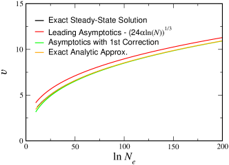
Figure 1: Exact quasi-static velocity compared to various approximations for the spatial continuum case, $a\to 0$, with $\alpha=0.3$, $D=1$, $r_{0}=1$.

III Dependence on $r_{0}$

To the order considered, $r_{0}$ has not entered into the calculated velocity. We can calculate the leading $r_{0}$ dependence by expanding Eq. (21) to quadratic order in $r_{0}$:

$$\ln N_{e}=\frac{v\gamma}{2D}-\frac{2}{3}\left(\frac{\gamma}{\delta}\right)^{3/2}\sim\frac{v^{3}}{24D^{2}\alpha}-\frac{r_{0}^{2}}{2v\alpha}$$ (24)

which induces a correction $\Delta v$ to the velocity of

$$\Delta v=\frac{4D^{2}r_{0}^{2}}{v^{3}}$$ (25)

so that $v$ increasing quadratically with $r_{0}$ to leading order. Note that the shift is small, of order $1/v$ even for $r_{0}$ of order $v$. Also, $r_{0}$ cannot be taken to be of order $v^{2}$, since then diffusion is relevant in the bulk. In Fig. 2 a comparison between formula (25) and numerical results is shown. The initial quadratic dependence is clearly seen. For large enough $r_{0}$ our formula fails. Indeed for very large $r_{0}$, the effect of the reaction gradient is suppressed, and the velocity should approach that of the (cutoff) Fisher equation with rate $r_{0}$ bd

$$v=2\sqrt{r_{0}D}\left(1-\frac{\pi^{2}}{\ln^{2}{N_{e}}}\right).$$ (26)

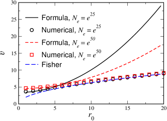
Figure 2: Comparison of the predicted $r_{0}$ dependence, Eq. (25), and numerical results for the spatial continuum limit $a\to 0$, with $\alpha=0.1$, $D=1$. Also included is the Fisher velocity, Eq. (26), where the graphs for the two $N_{e}$’s coincide on the scale of the figure.

IV The Continuum Problem, á la WKB

The fact that we could solve the linear problem exactly obscures the fact that most of the structure of the problem comes from the asymptotic properties of the solution. In fact, we can get essentially everything we require via a WKB treatment. Writing $\phi=e^{S}$, we get to leading order

$$DS^{\prime 2}+vS^{\prime}+\alpha y=0$$ (27)

where we have written $y=x+r_{0}/\alpha$ and the derivatives are w.r.t. $y$. Equation (27) defines $S^{\prime}$ implicitly in term of $y$. For small $y$, we get $S^{\prime}=-\alpha y/v$, so that $S=S_{0}-\alpha y^{2}/(2v)$. Matching to the bulk solution gives $S_{0}=r_{0}^{2}/(2v\alpha)\approx 0$, if we take $r_{0}$ to be order 1. Later, we will see what happens when $r_{0}$ is of order $v$. Now what is critical, as we saw above, is the turning point, since beyond this point $S^{\prime}$ turns complex, $\phi$ starts to oscillate, and so hits zero, which allows us to match to the post-cutoff solution. The turning point is given by the discriminant condition, which we can write as

$$\frac{d}{dS^{\prime}}[DS^{\prime 2}+vS^{\prime}+\alpha y]=0$$ (28)

or

$$S^{\prime}_{*}=-\frac{v}{2D}$$ (29)

Solving for the turning point $y_{*}$ gives us $y_{*}=v^{2}/(4D\alpha)$ which is consistent with the solution given above in section II, where the turning point occurs where the argument of the Ai function is zero. However, we do not actually need the value of the turning point, just that of $S^{\prime}$ there, namely $S^{\prime}_{*}$. Since, as we verify later, the turning point is close to the zero of the solution, the dominant contribution to the value of $\phi$ is $e^{S_{*}}$. This is given by

$$S_{*} = \int_{0}^{y_{*}}dy\,S^{\prime}=\int_{0}^{S^{\prime}_{*}}dS^{\prime}\,S^{\prime}\frac{dy}{dS^{\prime}}$$ (30)

$$= \int_{0}^{S^{\prime}_{*}}dS^{\prime}\,S^{\prime}[-(2DS^{\prime}+v)/\alpha]=-\frac{v^{3}}{24D^{2}\alpha}$$

Note that we did not need an explicit expression for $S^{\prime}(y)$, which is good, since in the lattice case we won’t have such an expression. This calculation is already enough to give us the leading asymptotics, since to leading exponential order $\phi(x_{c})=e^{S_{*}}$, or $S_{*}=-\ln N_{e}$, exactly what we got above. The origin of the correction lies in the fact that the zero lies a small distance beyond the turning point, namely $\xi_{0}\delta$, a result we need the Airy equation to derive. The real part of $S^{\prime}$ is fixed at $S^{\prime}_{*}$ beyond the turning point, so $S$ at the zero is $S_{*}-\xi_{0}\delta v/(2D)$, which we need to set equal to $-\ln N_{e}$. This gives us the correction derived above.

V The Lattice Problem

Now we are in a position to return to our lattice problem, Eq. (5). As above, in the bulk diffusion is irrelevant and the solution is the same as before. Close to the turning point, we linearize and expand $S(x\pm a)$ (even though we can’t expand $\phi(x\pm a)$),  bender ; rouzine and the WKB equation is

$$0=\frac{4D}{a^{2}}\sinh^{2}(aS^{\prime}/2)+vS^{\prime}+\alpha y$$ (31)

Already at this point, we get a nontrivial result. We can de-dimensionalize this equation by introducing $T=a/\ell S$, $z=y/\ell$, $\ell=v/(a\alpha)$ so that the equation reads

$$0=\frac{4D}{va}\sinh^{2}(T^{\prime}/2)+T^{\prime}+z$$ (32)

where the derivative is now w.r.t. $z.$ Thus, $S$ (i.e. $\ln N_{e}$) scales like $D/(\alpha a^{3})$ times a function of the dimensionless parameter $va/D$, so that the results for all $a$, (for a given $k$ and $D$) should lie on a universal curve. Furthermore, we see that $a$ is a singular perturbation as far as the large velocity limit goes rouzine , since no matter how small $a$ is, the parameter $va/D$ eventually goes to infinity.

Returning to Eq. (31), the turning point is given by the discriminant equation

$$0=\frac{2D}{a}\sinh(aS^{\prime}_{*})+v$$ (33)

which gives

$$S^{\prime}_{*}=\frac{1}{a}\ln\left(\sqrt{1+\frac{v^{2}a^{2}}{4D^{2}}}-\frac{va}{2D}\right)$$ (34)

Again, we need to calculate the change in $S$ from $y=0$ to the turning point $y_{*}$. This is given as above by

$$S_{*} = \int_{0}^{S^{\prime}_{*}}dS^{\prime}\,S^{\prime}\frac{dy}{dS^{\prime}}$$ (35)

$$= \int_{0}^{S^{\prime}_{*}}dS^{\prime}\,S^{\prime}[-(\frac{2D}{a}\sinh(aS^{\prime})+v)/\alpha]$$

$$= -\frac{2D}{\alpha a^{2}}S^{\prime}_{*}\cosh(aS^{\prime}_{*})+\frac{2D}{\alpha a^{3}}\sinh(aS^{\prime}_{*})-\frac{v(S^{\prime}_{*})^{2}}{2\alpha}$$

This then is the leading order WKB answer. Again, to get the correction, we need to examine the vicinity of the turning point more closely. We write

$$\phi(y)=e^{S^{\prime}_{*}y}\psi(y)$$ (36)

In the vicinity of the turning point, this removes the large variation of $\phi$ between lattice points, leaving us free to Taylor expand the rest. Substituting this into Eq. (5), we get

$$0 = \frac{D}{a^{2}}\left[e^{aS^{\prime}_{*}}\psi(y+a)+e^{-aS^{\prime}_{*}}\psi(y-a)-2\psi(y)\right]+vS^{\prime}_{*}\psi(y)+v\psi^{\prime}(y)+\alpha y\psi$$ (37)

$$= \frac{D}{a^{2}}\left[e^{aS^{\prime}_{*}}\left(\psi+a\psi^{\prime}+a^{2}\psi^{\prime\prime}/2\right)+e^{-aS^{\prime}_{*}}\left(\psi-a\psi^{\prime}+a^{2}\psi^{\prime\prime}/2\right)-2\psi\right]+vS^{\prime}_{*}\psi+v\psi^{\prime}+\alpha y\psi$$

$$= D\cosh(aS^{\prime}_{*})\psi^{\prime\prime}+\alpha(y-y_{*})\psi$$

Again, we get an Airy equation. This gives us the distance from the turning point to the zero of $\psi$, which is $\xi_{0}\delta_{a}$ where

$$\delta_{a}\equiv(\alpha/(D\cosh(aS^{\prime}_{*})))^{-1/3}$$ (38)

is the length scale of the Airy equation for the lattice problem. This gives us an additional contribution of $-S^{\prime}_{*}\xi_{0}\delta_{a}$ to $S$. Again, the solution for the velocity is just $\ln N_{e}=-S$, so that

$$\ln N_{e}=\left[\frac{2D}{a^{2}}S^{\prime}_{*}\cosh(aS^{\prime}_{*})-\frac{2D}{a^{3}}\sinh(aS^{\prime}_{*})+v(S^{\prime}_{*})^{2}/2\right]/\alpha-\xi_{0}S^{\prime}_{*}\left(\frac{\alpha}{D\cosh(aS^{\prime}_{*})}\right)^{-1/3}$$ (39)

Let us examine the various limits of the this expression. First, the continuum limit, $av/D\ll 1$. Then $S^{\prime}_{*}=-v/2D$, as in the continuum calculation, so that $aS^{\prime}\ll 1$. Then, $S_{*}=-(2D(S^{\prime}_{*})^{3}/3+v(S^{\prime}_{*})^{2}/2)/\alpha=-v^{3}/(24D^{2}\alpha)$, also exactly as in the continuum calculation. The correction term is $-S^{\prime}_{*}\xi_{0}(\alpha/D)^{-1/3}$, which also agrees.

Now, as we mentioned above, for any finite $a$, $av/D$ is eventually large for sufficiently large $N_{e}$. Then, $S^{\prime}_{*}=-\ln(va/D)/a$. This gives $S_{*}=v/(a^{2}\alpha)(-\ln(va/D)+1+\ln^{2}(va/D)/2)$. Now, for very large $va/D$, $S_{*}\approx-v\ln(va/D)/(a^{2}\alpha)$. However, this is only valid for $ln(va/D)\gg 2$. In fact, it is a reasonable (20%) approximation only for $\ln(va/D)$ bigger than 10, so that $v$ would be unreasonably large. Thus, a strict asymptotic expansion is of no use whatsoever. Over the range $5<x<11$, an excellent approximation of $\ln^{2}(x)/2+1-\ln(x)$ is $x/7.4$ (see Fig. 3).

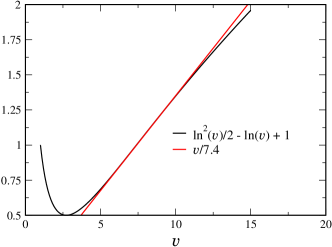
Figure 3: Comparison of the function $\ln^{2}(v)/2-\ln(v)+1$ and the linear approximation $v/7.4$

Thus, in the relevant range, $S_{*}\approx v^{2}/(7.4a\alpha D)$. Thus, while formally, to leading order

$$\ln N_{e}\approx v/(a^{2}\alpha)\ln^{2}(va/D)$$ (40)

or equivalently

$$v\approx a^{2}\alpha\ln(N_{e})/\ln^{2}(a^{3}\alpha\ln(N_{e})/D)$$ (41)

this is true only for astronomically large $N_{e}$. More useful, though phenomenological, is

$$v\approx\sqrt{7.4a\alpha D\ln N_{e}}$$ (42)

Thus, the velocity increases with $\alpha$, $D$ and $N_{e}$. Including the correction term, we get the effective approximation

$$v\approx\sqrt{7.4a\alpha D\ln N_{e}}-1.76\alpha^{1/3}D^{2/3}(\ln(N_{e}))^{-1/3}\ln(7.4a^{3}\alpha\ln(N_{e})/D)$$ (43)

Fig. 4 presents the case $a=1$.

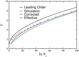
Figure 4: Velocity vs. $\ln(N_{e})$ for lattice spacing $a=1$, $\alpha=0.1$, $D=r_{0}=1$ from simulation, together with the various analytic approximations. The curve labeled “Leading Order” represents Eq. (35) and that labeled “Correction” represents Eq. (39). The curve labeled “Effective” represents Eq. (43).

We see that for $v$’s bigger than 4, the corrected approximation is excellent. The leading order approximation, however, is poor even for $\ln(N_{e})$ as unreasonably large as 100. The simplified effective approximation Eq. (43) is as good as the full corrected approximation for this range of $N_{e}$. The extremely simple Eq. (42) is as good as the leading order approximation. In Fig. 5, we present data for a number of values of $a$, ranging from 0 to 1, along with our analytic prediction. Again, the agreement is very good.

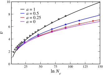
Figure 5: Velocity vs. $\ln(N_{e})$ for lattice spacings $a=1$, 0.5, 0.25, and 0, $\alpha=0.1$, $D=r_{0}=1$ from simulation, together with the analytic approximation Eq. (39)

In Fig. 6, we show the dependence on $\alpha$, the gradient of the reaction rate. We see that the rise in $v$ is quite steep at first, and then tapers off to an much slower rise. It should be noted how much an effect the correction term has, especially at larger $\alpha$. Nowhere does it look simply proportional to $\alpha$, as would naively appear from the leading order calculation, Eq. (40).

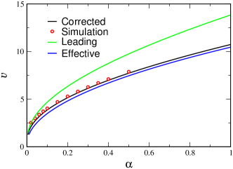
Figure 6: Velocity vs. $\alpha$ for lattice spacing $a=1$, $D=r_{0}=1$, $\ln(N_{e})=25$, from simulation, together with the leading-order and corrected analytic approximations, as in Fig. 4.

In Fig. 7, we show the dependence of $v$ on the diffusion constant, $D$. Again, the rise in $v$ is steep at small $D$, and grows essentially linear for large $D$. As $v/D$ is a decreasing function of $D$, for large $D$ the continuum limit is eventually valid. We see in fact that the continuum approximation, Eq. (23) works quite well over the entire range of $D$.

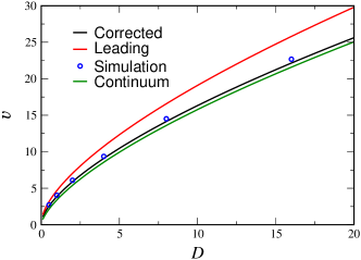
Figure 7: Velocity vs. $D$ for lattice spacing $a=1$, $\alpha=0.1$, $r_{0}=1$, $\ln(N_{e})=25$, from simulation, together with the leading-order and corrected analytic approximations, as in Fig. 4. Also included is the continuum approximation, Eq. (23).

VI Next-order WKB

To go further, we need to both improve our WKB solution and to extend our solution to the region $x>x_{c}$. Note that it is easy to check that we do not need to reconsider the diffusionless solution in the bulk, as the first-order correction to that solution is lower order (in terms of its ultimate effect on the velocity) than the correction we derive here. We first consider the next-order WKB solution. We write $\phi=e^{S_{0}+S_{1}}$, and get the next order WKB equation

$$\frac{2D}{a^{2}}\left[aS_{1}^{\prime}\sinh(aS_{0}^{\prime})+\frac{a^{2}}{2}S_{0}^{\prime\prime}\cosh(aS_{0}^{\prime})\right]+vS_{1}^{\prime}=0$$ (44)

with the solution

$$S_{1}=-\frac{1}{2}\ln\left(\frac{av}{2D}+\sinh(aS_{0}^{\prime})\right)+C_{1}$$ (45)

so that

$$\phi\approx(av/2D+\sinh(aS_{0}^{\prime}))^{-1/2}e^{C_{1}+S_{0}}$$ (46)

We have to match the solution to the bulk solution, which is approximately $e^{-\frac{\alpha y^{2}}{2v}}$. The matching area is defined by the requirement that on the one hand diffusion be irrelevant, so that $-S_{0}^{\prime}\approx\alpha y/v\ll\ln v$, or $y\ll v\ln v$, and on the other, $\phi$ is small, implying $y^{2}/v\gg 1$, or $y\gg v^{1/2}$. Thus to do the matching we can take $y\sim O(v)$. Neglecting the $\sinh$, we get from Eq. (46):

$$C_{1}=\frac{1}{2}\ln\left(\frac{va}{2D}\right),$$ (47)

and the WKB solution is,

$$\phi=e^{S_{0}}\left(1+\frac{2D}{va}\sinh(aS^{\prime})\right)^{-1/2}$$ (48)

We now need to match the WKB solution to the Airy solution of $\phi=e^{S_{*}^{\prime}(y-y_{*})}\psi$, where $\psi=C_{2}Ai((y_{*}-y)/\delta_{a})$. First we find the matching region. Clearly we need the argument of the Airy function to be large. Thus gives us that $y_{*}-y\gg\delta_{a}$. In the lattice limit, this reduces to $y_{*}-y\gg v^{-1/3}$, while in the continuum limit, we get $y_{*}-y\gg 1$. Near the turning point, $S_{0}^{\prime}\approx S_{*}^{\prime}+\delta_{a}^{-3/2}\sqrt{y_{*}-y}$. This is valid as long as $a\delta_{a}^{-3/2}\sqrt{y_{*}-y}\ll 1$, or $y_{*}-y\ll\delta_{a}^{3}/a^{2}$. Thus, we can match as long as $\delta_{a}\ll\delta_{a}^{3}/a^{2}$, which is uniformly true in the large $v$ limit. Approximating the Airy solution, we get

$$\phi \approx C_{2}e^{S_{*}^{\prime}(y-y_{*})}\textrm{Ai}\left((y_{*}-y)/\delta_{a}\right)$$ (49)

$$\approx \frac{1}{2\sqrt{\pi}}\delta_{a}^{1/4}(y_{*}-y)^{-1/4}C_{2}e^{S_{*}^{\prime}(y-y_{*})}e^{-\frac{2}{3}\left((y_{*}-y)/\delta_{a}\right)^{3/2}}$$

Approximating the WKB solution, we get

$$\phi \approx \left(1+\frac{2D}{va}\sinh(aS_{0}^{\prime}(y))\right)^{-1/2}e^{S_{0}(y)}$$ (50)

$$\approx \left(1+\frac{2D}{va}\left[\sinh(aS_{*}^{\prime})+a\cosh(aS_{*}^{\prime})\sqrt{\delta_{a}^{-3}(y_{*}-y)}\right]\right)^{-1/2}e^{S_{*}-S_{*}^{\prime}(y_{*}-y)-\frac{2}{3}\delta_{a}^{-3/2}(y_{*}-y)^{3/2}}$$

$$\approx \left(\frac{2D}{v}\cosh(aS_{*}^{\prime})\sqrt{\delta_{a}^{-3}(y_{*}-y)}\right)^{-1/2}e^{S_{*}-S_{*}^{\prime}(y_{*}-y)-\frac{2}{3}\delta_{a}^{-3/2}(y_{*}-y)^{3/2}}$$

Matching these two gives

$$C_{2}=\frac{\sqrt{2\pi v}}{D^{1/3}\alpha^{1/6}\cosh^{1/3}(aS_{*}^{\prime})}e^{S_{*}}$$ (51)

It is easy to verify that this agrees in the $a\rightarrow 0$ limit with the direct continuum calculation, Eq. (19).

VII Matching to $x>x_{c}$

Finally, we have to actually match to the solution for $x>x_{c}$. For $x>x_{c}$, we clearly cannot expand $\psi$ as we have done, since the falloff of $\phi$ is much faster than $exp(-S^{\prime}_{*}x)$. We can understand what happens by considering doing the expansion of $\psi$ to one more order. The higher derivative induces a boundary layer at $x_{c}$, which serves to insure continuity of the second derivative, but leaves the lower-order derivatives untouched. As we expand to higher and higher order, there are more and more boundary-layer modes, which we have to match. The correct way to do the matching then is via a Wiener-Hopf (WH) procedure. To do the WH, we consider our problem in the immediate vicinity of $x_{c}$. Here, we can approximate $\alpha y$ by $\alpha y_{c}$, since as we have seen, $y_{c}$ is large. Now we have a constant coefficient difference equation, which we can solve via WH.

Let us do this first for the continuum problem for practice, since here we know the correct answer. The approximate equation is

$$D\phi^{\prime\prime}+v\phi^{\prime}+\alpha y_{c}\theta(y_{c}-y)\phi=0$$ (52)

Writing $\phi=\phi_{L}+\phi_{R}$ and Fourier transforming, we get

$$-Dq^{2}(\phi_{L}+\phi_{R})+ivq(\phi_{L}+\phi_{R})+\alpha y_{c}\phi_{L}=0$$ (53)

or equivalently

$$(-Dq^{2}+ivq)\phi_{R}=-(-Dq^{2}+ivq+\alpha y_{c})\phi_{L}$$ (54)

The right-hand operator $R(q)=-Dq^{2}+ivq$ has two zeros, one at $q=0$ and one at $q=iv/D$, but $\phi_{R}$ has a pole only at $q=q_{R}=iv/D$. The left-hand operator $L(q)=-Dq^{2}+ivq+\alpha y_{c}$ has two essentially degenerate zeros, close to $q=iv/(2D)$, both of which are represented as poles in $\phi_{L}$. Thus, we rewrite the equation as follows

$$(q-q_{R})\phi_{R}=-\frac{L(q)(q-q_{R})}{R(q)}\phi_{L}$$ (55)

Now, the left-hand side of the equation has no zeros or poles below the line $\Im{q}=v/D$, and the right-hand side of the equation has no zero or poles above, so they must both be equal to a constant, $C$. Thus,

$$\phi_{R} = \frac{C}{q-q_{R}}$$

$$\phi_{L} = -\frac{CR(q)}{L(q)(q-q_{R})}=-\frac{Cq}{(q-q_{+})(q-q_{-})}$$ (56)

where $q_{\pm}$ are the two nearly degenerate roots of $L(q)$,

$$q_{\pm}=\frac{iv}{2D}\pm\Delta$$ (57)

with $\Delta=\frac{\sqrt{-v^{2}+4D\alpha y_{c}}}{2D}$ small. Fourier transforming back, we get

$$\phi_{R} = iCe^{-v(y-y_{c})/D}$$

$$\phi_{L} = iC\left[\frac{q_{+}}{q_{+}-q_{-}}e^{iq_{+}(y-y_{c})}+\frac{q_{-}}{q_{-}-q_{+}}e^{iq_{-}(y-y_{c})}\right]$$ (58)

Examining $\phi_{R}$, we find that $iC=1/N_{e}$. Turning to $\phi_{L}$, we found above that $y_{c}\approx v^{2}/(4\alpha D)-\xi_{0}\delta$, so

$$\Delta\approx\sqrt{-\alpha\xi_{0}\delta/D}$$ (59)

Now, as long as $(y-y_{c})\Delta\ll 1$, we can write

$$\phi_{L}=\frac{e^{-v(y-y_{c})/(2D)}}{N_{e}}\left[1-\frac{v}{2D}(y-y_{c})\right]$$ (60)

We now have to match this to the Airy function. Putting $y_{c}=v^{2}/(4D\alpha)-\xi_{0}\delta-y_{1}$, we find that

$$\phi \approx Ae^{-vy_{c}/2D}e^{-v(y-y_{c})/(2D)}\text{Ai}^{\prime}(\xi_{0})\left(\frac{y_{1}-(y-y_{c})}{\delta}\right)$$ (61)

$$= Ae^{-vy_{c}/2D}e^{-v(y-y_{c})/2D}\frac{\text{Ai}^{\prime}(\xi_{0})y_{1}}{\delta}\left(1-\frac{y-y_{c}}{y_{1}}\right)$$

Comparing the two results we find $y_{1}=2D/v$, and

$$Ae^{-vy_{c}/2D}\frac{2D\text{Ai}^{\prime}(\xi_{0})}{v\delta}=\frac{1}{N_{e}}$$ (62)

or

$$\ln N_{e} = -\frac{2}{3}\frac{v^{3}}{(4D\alpha)^{3/2}}\left(\frac{D}{\alpha}\right)^{-1/2}+\frac{v^{3}}{8D^{2}\alpha}-\frac{v\xi_{0}\delta}{2D}-1-\frac{1}{2}\ln 4\pi-\frac{1}{4}\ln\left(\frac{\gamma}{\delta}\right)-\ln\left(\frac{2D\text{Ai}^{\prime}(\xi_{0})}{v\delta}\right)$$ (63)

$$= \frac{v^{3}}{24D^{2}\alpha}-\frac{v\xi_{0}}{2(D^{2}\alpha)^{1/3}}-\ln\left(\text{Ai}^{\prime}(\xi_{0})2e\sqrt{2\pi}D^{1/3}\alpha^{1/6}v^{-1/2}\right)$$

This can be shown to agree with the direct asymptotic solution of Eq. II.

Now we do the same for the lattice problem. Again, after setting $\alpha y=\alpha y_{c}$, the equation has the form

$$R(q)\phi_{R}=-L(q)\phi_{L}$$ (64)

where

$$R(q) = -\frac{4D}{a^{2}}\sin^{2}\frac{aq}{2}+ivq$$

$$L(q) = R(q)+\alpha y_{c}$$ (65)

$R(q)$ has two pure imaginary roots, one at $q=0$ and the other with positive imaginary part, $\kappa_{R}$. Since we cannot allow $\phi_{R}$ to become negative, the dominant solution for large $x$ must be controlled by this positive imaginary root, leading to a pure exponential decay. Only this root and the complex roots which decay faster ($\Im q>\kappa_{R}$) are then permissible. As in the continuum, since $y_{c}$ is close to $y_{*}$, $L(q)$ has a pair of almost degenerate roots, $q_{\pm}$ with small real parts and a positive imaginary part smaller than $\kappa_{R}$. To match to the $Ai$ solution, this must be the dominant contribution for large negative $y-y_{c}$, so the only acceptable roots are those with $\Im q\leq\Im q_{\pm}$. We therefore decompose $R(q)$ and $L(q)$ into two factors, one with its zeros below $i\kappa_{R}$, which we label by a “$B$” superscript, and the other with its zeros above (or equal), which we label by “$U$”. Formally,

$$R(q) = R^{U}(q)R^{B}(q)$$

$$L(q) = L^{U}(q)L^{B}(q)$$ (66)

where

$$R^{U}(q) = \prod_{i}\left(1-\frac{q}{q^{U}_{R,i}}\right)$$

$$R^{B}(q) = ivq\prod_{i}\left(1-\frac{q}{q^{B}_{R,i}}\right)$$

$$L^{U}(q) = \alpha y_{c}\prod_{i}\left(1-\frac{q}{q^{U}_{L,i}}\right)$$

$$L^{B}(q) = \left(1-\frac{q}{q_{+}}\right)\left(1-\frac{q}{q_{-}}\right)\prod_{i}\left(1+i\frac{q}{q^{B}_{L,i}}\right)$$ (67)

We have chosen to explicitly break out the factors relating to $q_{\pm}$ in $L^{B}$ since they will play an essential role in the following, and the factor $ivq$ in $R^{B}$ so that the correct behavior at $q=0$ is maintained. Then, via the standard Wiener-Hopf argument,

$$\phi_{R}(q) = C\frac{L^{U}}{R^{U}}$$

$$\phi_{L}(q) = -C\frac{R^{B}}{L^{B}}$$ (68)

It is easiest to proceed if we regularize the problem by effectively discretizing time, replacing the $ivq$ term in the operators $L$, $R$ by $ivn_{t}/a\sin(qa/n_{t})$ where $n_{t}$ is some large integer. Then, the operators become polynomials of order $2n_{t}$ in the variable $e^{iqa/n_{t}}$. Further study reveals that $R^{U}$ then has $n_{t}-1$ zeros, $R^{B}$ has $n_{t}+1$, $L^{U}$ has $n_{t}-2$ zeros, and $L^{B}$ has $n_{t}+2$. Thus, $\phi_{L}$ behaves as $q^{-1}$ for large $q$, and so

$$\phi_{L}(y_{c})=-i\lim_{q\to\infty}q\phi_{L}(q)=-Cvq_{+}q_{-}\prod\frac{q^{B}_{L,i}}{q^{B}_{R,i}}$$ (69)

so that

$$C=-\frac{1}{N_{e}vq_{+}q_{-}}\prod\frac{q^{B}_{R,i}}{q^{B}_{L,i}}$$ (70)

so that

$$\phi_{L}(q)=\frac{iq}{N_{e}(q-q_{+})(q-q_{-})}\prod_{i}\frac{q-q^{B}_{R,i}}{q-q^{B}_{L,i}}$$ (71)

If $y$ is not too close to $y_{c}$, only the two dominant modes, which we have labeled $q_{\pm}=-iS^{\prime}_{*}\pm\Delta$ survive, and we get

$$\phi_{L}(y)\approx\frac{1}{N_{e}}\prod_{i}\frac{-iS^{\prime}_{*}-q^{B}_{R,i}}{-iS^{\prime}_{*}-q^{B}_{L,i}}e^{S^{\prime}_{*}(y-y_{c})}\left(1+\sum_{j}\left(\frac{-S^{\prime}_{*}}{-S^{\prime}_{*}+iq^{B}_{R,j}}-\frac{-S^{\prime}_{*}}{-S^{\prime}_{*}+iq^{B}_{L,j}}\right)+S^{\prime}_{*}(y-y_{c})\right)$$ (72)

This is seen to reproduce the continuum results above when $a\to 0$. Now we must match Eq. (72) to our Airy function solution to Eq. (37). Actually, to the order we are working, we must take into consideration the first lattice correction to the Airy equation, namely

$$\frac{Da\sinh(aS^{\prime}_{*})}{3}\psi^{\prime\prime\prime}+D\cosh(aS^{\prime}_{*})\psi^{\prime\prime}+\alpha(y-y_{*})\psi=0\ .$$ (73)

The (first order) approximate solution to this is

$$\psi(y)\approx C_{2}\left(1+\frac{a\tanh(aS^{\prime}_{*})}{12\delta_{a}^{3}}(y-y_{*})^{2}\right)\text{Ai}\left(-\frac{y-y_{*}}{\delta_{a}}+\frac{a\tanh(aS^{\prime}_{*})}{6\delta_{a}}\right)\ .$$ (74)

Substituting $y_{c}=y_{*}-\xi_{0}\delta_{a}-y_{1}$, with $y_{1}/\delta_{a}\ll 1$, we find

$$\phi(y)\approx C_{2}e^{S^{\prime}_{*}(y_{c}-y_{*})}e^{S^{\prime}_{*}(y-y_{c})}\frac{Ai^{\prime}(\xi_{0})}{\delta_{a}}\left[y_{1}+\frac{a\tanh(aS^{\prime}_{*})}{6}-(y-y_{c})\right]$$ (75)

Thus gives us

$$y_{1}=-\frac{a\tanh(aS^{\prime}_{*})}{6}+\frac{1}{-S^{\prime}_{*}}+\sum_{j}\left(\frac{1}{-S^{\prime}_{*}+iq^{B}_{R,j}}-\frac{1}{-S^{\prime}_{*}+iq^{B}_{L,j}}\right)$$ (76)

A graph of $y_{1}$ as a function of $v$ is presented in Fig. 8, together with the continuum result. We see that whereas $y_{1}$ falls with $v$ in the continuum, due to the lattice correction to the Airy equation, the lattice $y_{1}$ approaches a constant for large $v$. In fact, at large $v$, all the $q$’s can be calculated analytically, and the some performed. This calculation shows that to leading order, both the sum over the right and left modes approaches $1/2$, with the difference vanishing as $v\to\infty$. The lattice $y_{1}$ is dominated by the lattice correction to the Airy equation, which approaches the constant $a/6$ for large $v$. Included in this figure is a comparison between analytical and numerical results. We see that as expected the analytic result approaches the numerical results are $v$ increases, being quite accurate everywhere.

The numerical results presented in this graph, in contrast to those presented throughout the rest of this paper, were not obtained through direct numerical simulation of the time-dependent equations, due to the high accuracy required to perform the comparison with the theory. Our direct numerical simulations were performed via a straightforward Euler simulation, which is only first-order accurate in the time step. Extremely small time-steps would have been required to obtain the requisite accuracy. Instead, we solved the linearized steady-state equation directly. As opposed to $v(N_{e})$, which requires a full nonlinear solution, $y_{1}(v)$ is determined solely by the linearized equation. The procedure we employed was as follows: The solution past the cutoff was written as a linear superposition of the allowed modes, corresponding to the roots $q_{R}^{U}$. The solution to the left of some conveniently chosen $y_{\ell}$ was written as a linear superposition of modes, with the reaction rate set at the constant value $r(y_{\ell})=r(y_{c})-\alpha(y_{c}-y_{\ell})$. The steady-state equations between $y_{\ell}$ and $y_{c}$ were written as a banded matrix, acting on the three sets of unknowns: the coefficients of the pre-$y_{\ell}$ modes; the values of the field between $y_{\ell}$ and $y_{c}$; and the coefficients of the post-$y_{c}$ modes. This matrix depends on the two parameters $v$ and $r(y_{c})$. Now the pre-$y_{\ell}$ modes include two real modes, corresponding to the two solutions of the quadratic equation for $S^{\prime}$. In order to match the Airy function behavior, the faster of these two modes must not be present. This is an eigenvalue condition of $r(y_{c})$ for a given $v$. From $r(y_{c})$ we can back out $y_{1}$, as presented in the figure. This procedure converges quadratically in the discretization $\Delta y$. The convergence with respect to $y_{\ell}$ is exponentially rapid, and presented no problem. A comparison of the answers obtained in this manner with that obtained by direct numerical simulation, at low values of $v$ for which the latter calculation was feasible, verified the validity of this alternate approach. This new approach also sheds an interesting light on the selection problem inherent in the linearized steady-state equation.

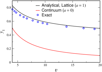
Figure 8: Large $v$ analytic approximations for $y_{1}$ vs. velocity for $\alpha=0.1$, $r_{0}=1$, $D=1$, both for lattice spacing $a=1$, and for the continuum limit, together with results from simulation.

All that remains is to put everything together and construct the full approximation for the velocity as a function of the cutoff, $N_{e}$. As we have seen, in the matching region, the WH $\phi_{L}$ has the same functional form as the Airy solution, once $y_{1}$ is picked appropriately as described above, the two solutions differing only in normalization. Setting the normalization factors equal then fixes $1/N_{e}$ in terms of our previously calculated $C_{2}$, (see Eq. (51)). Doing this gives

$$\ln N_{e}=-S_{*}+S^{\prime}_{*}(\xi_{0}\delta_{a}+y_{1})-\ln\left(\sqrt{2\pi v/\alpha}{\delta_{a}}^{-1}\right)-\ln\left(\frac{{\text{Ai}}^{\prime}(\xi_{0})}{\delta_{a}(-S^{\prime}_{*})}\prod\frac{-iS^{\prime}_{*}-q^{B}_{L,i}}{-iS^{\prime}_{*}-q^{B}_{R,i}}\right)\ .$$ (77)

In Fig. 9 we present the ratio of $N_{e}$ as predicted by this formula to the results of numerical simulation. We see that the ratio appears to approach unity as $v$ increases. Together with this is shown the ratio of $N_{e}$ from the lower order formula, Eq. (39). This formula, while it does better at small $v$, is seen to diverge from the exact answer with increasing $v$.

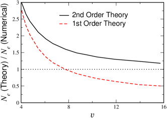
Figure 9: Ratio of $N_{e}$ as predicted by Eq. (77) to the exact $N_{e}$ from numerical simulation for $D=1$, $\alpha=0.1$, $a=1$. Also shown is the ratio of $N_{e}$ as predicted from the lower-order result, Eq. (39) to the exact $N_{e}$.

VIII Conclusions

In summary, we have presented an analytical study of the velocity of Fisher fronts in the presence of a gradient. This study exploits the fact that the velocity diverges as the local density of reactants increases. This divergence is one of the signposts of the extreme sensitivity to fluctuations of this class of models. One of the most surprising consequences of this sensitivity is the different order of the divergence in the continuum versus the lattice model; whereas the velocity of the front in the continuum limit diverges as $\ln^{1/3}(N)$,on the lattice, the velocity effectively diverges as $\sqrt{\ln{N}}$. The relative insensitivity to the details of the matching to the post-cutoff regime is another characteristic feature of this problem. It is clear, for example, that the leading order results are completely independent of the post-cutoff dynamics. Even the next order, which formally does depend on matching to the solution past $x_{c}$, is in fact only very weakly modified by the “R” modes arising from this region. This lack of strong dependence is no doubt a major part of the reason that the phenomenological cutoff theory works as well as it does in describing the stochastic model.

Obviously, the cutoff MFE approach cannot capture any of the truly stochastic features of the original Markov model. Thus, the next step in our overall program for understanding fronts in gradients must involve adding back in the residual effects of finite particle number fluctuations to the cutoff theory. Exactly how to do this is already unclear in the simpler case of the Fisher equation front, where it has proven difficult to come up with a simple explanation for the numerically determined front diffusion constant. bd2 ; debrata . The first question to be answered for the gradient case is whether the front can be described as simply diffusing (albeit with an anomalous diffusion constant) or whether the fluctuation effects perhaps lead to even stronger stochasticity. We hope to report on this issue in a future publication.

- (1) W. van Saarloos, Phys. Rep., 386, 29 (2003).
- (2) D. A. Kessler, J. Koplik, and H. Levine, Adv. Phys. 37, 255 (1988).
- (3) A. I. Kolmogorov, I. Petrovsky, and N. Piscounov, Moscow Univ. Bull. Math. A 1, 1 (1937).
- (4) J. Mai, I. M. Sokolov and A. Blumen, Phys. Rev. Lett. 77, 4462 (1996).
- (5) E. Ben-Jacob et al Physica D, 14, 348 (1985).
- (6) E. Brunet and B. Derrida, Phys. Rev. E 56, 2597 (1997)
- (7) U. Ebert and W. van Saarloos, Phys. Rev. Lett. 80, 1650 (1998).
- (8) D. A. Kessler, Z. Ner, and L. M. Sander, Phys. Rev. E 58, 107 (1998).
- (9) L. Pechenik, H. Levine, Phys. Rev. E 59, 3893 (1999).
- (10) D. A. Kessler and H. Levine, Nature 394, 556 (1998).
- (11) E. Cohen, D. A. Kessler and H. Levine, Phys. Rev. Lett. 94, 158302 (2005).
- (12) Experimental propagation against a gradient appears in D. Giller, et al., Phys. Rev. B63, 220502(R) (2001).
- (13) R. A. Fisher, Annual Eugenics 7, 355 (1937).
- (14) L. S. Tsimring, H. Levine and D. A. Kessler, Phys. Rev. Lett. 76, 4440 (1996); D. Ridgway, H. Levine, and L. Tsimring , J. Stat. Phys. 87, 519 (1997).
- (15) I. M. Rouzine, J. Wakeley, and J. M. Coffin, PNAS. 100, 587 (2003).
- (16) This naive mean-field theory was studied in M. Freidlin, in P. L. Hennequin, ed., Lecture Notes in Mathematics 1527 (Springer-Verlag, Berlin, 1992).
- (17) The chemical context suggests the continuum limit of the absolute model; the Darwinian problem gives rise to the discrete-space version of the quasi-static problem,
- (18) E. Brener, H. Levine, and Y. Tu, Phys. Rev. Lett. 66, 1978 (1991).
- (19) T. B. Kepler and A. S. Perelson, PNAS, 92, 8219 (1995).
- (20) L. I. Slepyan, Dokl. Akad. Nauk SSSR 258-259, 561 (1981) [Sov. Phys. Dokl. 26, 538 (1981)].
- (21) C. M. Bender and S. A. Orszag, Advanced Mathematical Methods for Scientists and Engineers I, (Springer, New York, 1999), Section 5.3.
- (22) E. Brunet and B. Derrida, J. Stat. Phys. 103 269 (2001).
- (23) D. Panja, Phys. Rev. E 68, 065202(R) (2003).