Transition to Instability in a Periodically Kicked Bose-Einstein Condensate on a Ring

Abstract

A periodically kicked ring of a Bose-Einstein condensate is considered as a nonlinear generalization of the quantum kicked rotor, where the nonlinearity stems from the mean field interactions between the condensed atoms. For weak interactions, periodic motion (anti-resonance) becomes quasiperiodic (quantum beating) but remains stable. There exists a critical strength of interactions beyond which quasiperiodic motion becomes chaotic, resulting in an instability of the condensate manifested by exponential growth in the number of noncondensed atoms. In the stable regime, the system remains predominantly in the two lowest energy states and may be mapped onto a spin model, from which we obtain an analytic expression for the beat frequency and discuss the route to instability. We numerically explore parameter regime for the occurrence of instability and reveal the characteristic density profile for both condensed and noncondensed atoms. The Arnold diffusion to higher energy levels is found to be responsible for the transition to instability. Similar behavior is observed for dynamically localized states (essentially quasiperiodic motions), where stability remains for weak interactions but is destroyed by strong interactions.

I Introduction

The $\delta$-kicked rotor is a textbook paradigm for the study of classical and quantum chaos reichl . In the classical regime, increasing kick strengths destroy regular periodic or quasiperiodic motions of the rotor and lead to the transition to chaotic motions, characterizing by diffusive growth in the kinetic energy. In quantum mechanics, chaos is no longer possible because of the linearity of the Schrödinger equation and the motion becomes periodic (anti-resonance), quasiperiodic (dynamical localization), or resonant (quantum resonance) QKR ; anti-res . Experimental study of these quantum phenomena have been done with ultra-cold atoms in periodically pulsed optical lattices raizen . However, most of previous investigations have been focused on single particle systems and the effects of interaction between particles have not received much attention NLSE ; zoller .

In recently years, the realization of Bose-Einstein condensation (BEC) BEC of dilute gases has opened new opportunities for studying dynamical systems in the presence of many-body interactions. One can not only prepare initial states with unprecedented precision and pureness, but also has the freedom of introducing interactions between the particles in a controlled manner. A natural question to ask is how the physics of the quantum kicked rotor is modified by the interactions. In the mean field approximation, many-body interactions in BEC are represented by adding a nonlinear term in the Schrödinger equation review (such nonlinear Schrödinger equation also appears in the context of nonlinear optics nonoptics ). This nonlinearity makes it possible to bring chaos back into the system, leading to instability (in the sense of exponential sensitivity to initial conditions) of the condensate wave function instability . The onset of instability of the condensate can cause rapid proliferation of thermal particles castin that can be observed in experiments ketterle . It is therefore important to understand the route to chaos with increasing interactions. This problem has recently been studied for the kicked BEC in a harmonic oscillator zoller .

In Ref. zhang1 , we have investigated the quantum dynamics of a BEC with repulsive interaction that is confined on a ring and kicked periodically. This system is a nonlinear generalization of the quantum kicked rotor. From the point of view of dynamical theory, the kicked rotor is more generic than the kicked harmonic oscillator, because it is a typical low dimensional system that obeys the KAM theorem, while the kicked harmonic oscillator is known to be a special degenerate system out of the framework of the KAM theorem liu1 . It is very interesting to understand how both quantum mechanics and mean field interaction affect the dynamics of such a generic system.

In this paper, we extend the results of Ref. zhang1 , including a more detailed analysis of the model considered there as well as new phenonmena. We will focus our attention on the relatively simpler case of quantum anti-resonance, and show how the state is driven towards chaos or instability by the mean field interaction. The paper is orgnaized as follows: Section II lays out our physical model and its experimental realization. Section III is devoted to the case of weak interactions between atoms. We find that weak interactions make the periodic motion (anti-resonance) quasiperiodic in the form of quantum beating. However, the system remains predominantly in the lowest two energy levels and analytic expressions for the beating frequencies are obtained by mapping the system onto a spin model. Through varying the kick period, we find the phenomenon of anti-resonance may be recovered even in the presence of interactions. The decoherence effects due to thermal noise are discussed. Section IV is devoted to the case of strong interactions. It is found that there exists a critical strength of interactions beyond which quasiperiodic motion (quantum beating) are destroyed, resulting in a transition to instability of the condensate characterized by an exponential growth in the number of noncondensed atoms. Universal critical behavior for the transition is found. We show that the occurrence of instability corresponds to the process of Arnold diffusion, through which the state can penetrate through the KAM tori and escape to high energy levels Arnold . We study nonlinear effects on dynamically localized states that may be regarded as quasiperiodic hog . Similar results are obtained in that localization remians for sufficiently weak interactions but become unstable beyond a critical strength of interactions. Section V consists of conclusions.

II Physical model: Kicked BEC on a ring

Although the results obtained in this paper are common properties of systems whose dynamics are governed by the nonlinear Schrödinger equation, we choose to present them here for a concrete physical model: a kicked BEC confined on a ring trap, where the physical meanings of the results are easy to understand. The description of the dynamics of this system may be divided into two parts: condensed atoms and non-condensed atoms.

II.1 Dynamics of condensed atoms: Gross-Pitaevskii equation

Consider condensed atoms confined in a toroidal trap of radius $R$ and thickness $r$, where $r\ll R$ so that lateral motion is negligible and the system is essentially one-dimensional ring . The dynamics of the BEC is described by the dimensionless nonlinear Gross-Pitaveskii (GP) equation,

$$i\frac{\partial}{\partial t}\psi=\left(-\frac{1}{2}\frac{\partial^{2}}{\partial\theta^{2}}+g\left|\psi\right|^{2}+K\cos\theta\delta_{t}(T)\right)\psi,$$ (1)

where $g=8NaR/r^{2}$ is the scaled strength of nonlinear interaction, $N$ is the number of atoms, $a$ is the $s$-wave scattering length, $K$ is the kick strength, $\delta_{t}(T)$ represents $\sum\limits_{n}\delta\left(t-nT\right)$, $T$ is the kick period, and $\theta$ denotes the azimuthal angle. The length and the energy are measured in units $R$ and $\frac{\hbar^{2}}{mR^{2}}$, respectively. The wavefunction $\psi\left(\theta,t\right)$ has the normalization $\int_{0}^{2\pi}\left|\psi\right|^{2}d\theta=1$ and satisfies periodic boundary condition $\psi\left(\theta,t\right)=\psi\left(\theta+2\pi,t\right)$.

Experimentally, the ring-shape potential may be realized using two 2D circular “optical billiards” with the lateral dimension being confined by two plane optical billiards billiard , or optical-dipole traps produced by red-detuned Laguerre-Gaussian laser beams of varying azimuthal mode index ringexp . The $\delta$-kick may be realized by adding potential points along the ring with an off-resonant laser raizen , or by illuminating the BEC with a periodically pulsed strongly detuned running wave laser in the lateral direction whose intensity $I$ is engineered to $I=I_{0}+I_{1}x/R$ Meck . In the experiment, we have the freedom to replace the periodic modulation $\cos\left(\theta\right)$ of the kick potential with $\cos\left(j\theta\right)$, where $j$ is an integer. Such replacement revises the scaled interaction constant $g$ and kicked strength $K$, but will not affect the results obtained in the paper. The interaction strength $g$ may be adjusted using a magnetic field-dependent Feshbach resonance or the variation of the number of atoms Feshbach .

II.2 Dynamics of non-condensed atoms: Bogoliubov equation

The deviation from the condensate wave function is described by Bogoliubov equation that is obtained from a linearization around GP equation castin . In Castin and Dum’s formalism, the mean number of noncondensed atoms at zero temperature is described by $\langle\delta\hat{N}(t)\rangle=\sum_{k=1}^{\infty}\langle v_{k}(t)|v_{k}(t)\rangle$, where $v_{k}(t)$ are governed by

$$i\frac{d}{dt}\left(\!\begin{array}[]{c}u_{k}\\ v_{k}\end{array}\!\right)=\left(\!\begin{array}[]{cc}H_{1}&H_{2}\\ -H_{2}^{\ast}&\!-H_{1}^{\ast}\end{array}\!\right)\!\left(\!\begin{array}[]{c}u_{k}\\ v_{k}\end{array}\!\right),$$ (2)

where $H_{1}=\hat{p}^{2}/2+g|\psi|^{2}-\mu+gQ|\psi|^{2}Q+K\cos\theta\delta_{t}(T),$ $\!H_{2}=gQ\psi^{2}Q^{\ast}$, $\mu$ is the chemical potential of the ground state, $\psi$ is the ground state of GP equation and the projection operators $Q$ are given by $Q=1-|\psi\rangle\langle\psi|.$

The number of noncondensed atoms describes the deviation from condensate wavefunction and its growth rate characterizes the stability of the condensate. If the motion of the condensate is stable, the number of noncondensed atoms grows at most polynomially with time and no fast depletion of the condensate is expected. In contrast, if the motion of the condensate is chaotic, the number of noncendensed atoms diverges exponentially with time and the condesate may be destroyed in a short time. Therefore the rate of growth of the noncondensed atoms number is similar the Lyapunov exponent for the divergence of trajectories in phase space for classical systems zoller .

III Weak Interactions: Anti-Resonance and Quantum Beating

In this section, we focus our attention on the case of quantum anti-resonance, and show how weak interactions between atoms modify the dynamics of the condensate. Quantum anti-resonace is a single particle phenomenon characterized by periodic recurrence between two different states, and its dynamics may be described by Eq. (1) with parameters $g=0$ and $T=2\pi$ anti-res .

III.1 Quantum Beating

In a non-interacting gas, the energy of each particle oscillates between two values because of the periodic recurrence of the quantum states. In the presence of interactions, single particle energy loses its meaning and we may evaluate the mean energy of each particle

$$E(t)=\int_{0}^{2\pi}d\theta\psi^{\ast}\left(-\frac{1}{2}\frac{\partial^{2}}{\partial\theta^{2}}+\frac{1}{2}g\left|\psi\right|^{2}\right)\psi.$$ (3)

To determine the evolution of the energy, we numerically integrate Eq.(1) over a time span of $100$ kicks, using a split-operator method split , with the initial wavefunction $\psi$ being the ground state $\psi\left(\theta,0\right)=1/\sqrt{2\pi}$. After each kick, the energy $E(t)$ is calculated and plotted as shown in Fig.1.

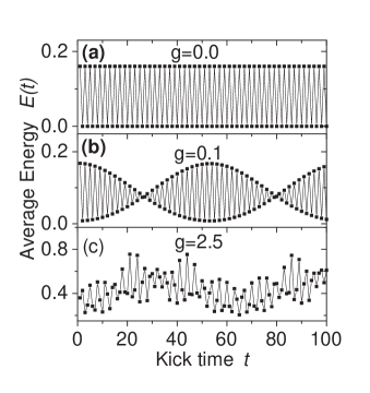
Figure 1: Plots of average energy $E(t)$ versus the number of kicks $t$ for three values of $g$. The kick strength $K=0.8$.

In the case of non-interaction (Fig.1(a) $g=0$), we see that the energy $E(t)$ oscillates between two values and the oscillation period is $2T$, indicating the periodic recurrence between two states (anti-resonance).

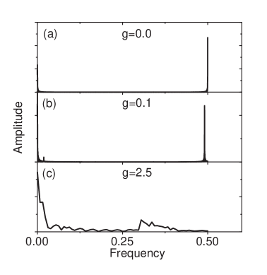
Figure 2: Fourier transformation of the energy evolutions in Fig.1. The Unit for the frequency is $1/T$.

The energy oscillation with weak interaction ($g=0.1$) in Fig.1(b) shows a remarkable difference from that for non-interaction case. We see that the amplitude of the oscillation decreases gradually to zero and then revives, similar to the phenomena of beating in classical waves. Clearly, it is the interactions between atoms in BEC that modulate the energy oscillation and produce the phenomena of quantum beating. As we know from classical waves, there must be two frequencies, oscillation and beat, to create a beating. These two frequencies are clearly seen in Fig.2 that is obtained through Fourier Transform of the energy evolutions in Fig.1. For the non-interaction case (Fig.2(a)), there is only the oscillation frequency $f_{osc}=0.5/T$, corresponding to one oscillation in two kicks. The interactions between atoms develop a new beat frequency $f_{beat}$, as well as modify the oscillation frequency $f_{osc}$, as shown in Fig.2(b).

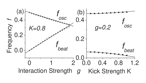
Figure 3: Plots of beat and oscillation frequencies versus the interaction strength (a) and kick strength (b), where the scatters are the results from numerical simulation using GP equation and lines from analytic expression Eqs. (15) and (16).

In Fig. 3, these two frequencies are plotted with respect to different interacting constant $g$ and kick strength $K$. We see that both beat and oscillation frequencies vary near linearly with reapect to the interaction strength $g$. More interestingly, the two frequencies satisfy a conservation relation

$$f_{osc}+f_{beat}/2=1/2.$$ (4)

For a strong interaction [Fig.1(c)], i.e., $g\geq 1.96$, we find that the energy’s evolution demonstrates an irregular pattern, clearly indicating the collapse of the quasiperiodic motion and the occurrence of instability. The corresponding Fourier transformation of the energy evolution (Fig.2(c)) has no sharp peak. This transition to instability will be discussed in Section IV in details.

III.2 Spin model

The phenomena of quantum beating can be understood by considering a two-mode approximation liu2 to the GP equation. In this approximation, condensed atoms can only effectively populate the two lowest second quantized energy modes. The validity of this two-mode model is justified by the following facts which are observed in the numerical simulation. First, the total energy of the condensate is quite small so that we can neglect the population at high energy modes and keep only the states with quantized momentums $0$ and $\pm 1$. Second, the total momentum of the condensate is conserved during the evolution. Therefore the populations of the states with momentum $\pm 1$ are same if the initial momentum of the condensate is zero (the ground state).

Here we consider a quantum approach of this two-mode model, which yields an effective spin Hamiltonian in the mean field approximation. By considering the conservation of parity we may write the Boson creation operator for the condensate as

$$\hat{\psi}^{\dagger}=\frac{1}{\sqrt{2\pi}}\left(\hat{a}^{\dagger}+2\hat{b}^{\dagger}\cos\theta\right)$$ (5)

where $\hat{a}^{\dagger}$ and $\hat{b}^{\dagger}$ are the creation operators for the ground state and the first excited states, satisfying the commutation relation $\left[\hat{a},\hat{a}^{\dagger}\right]=1$, $\left[\hat{b},\hat{b}^{\dagger}\right]=1$, and particle number conservation $\hat{a}^{\dagger}\hat{a}+\hat{b}^{\dagger}\hat{b}=N$.

Substituting Eq. (5) into the many-body Hamiltonian of the system

$$\hat{H} = \int_{0}^{2\pi}d\theta\left(\hat{\psi}^{\dagger}\left(-\frac{1}{2}\frac{\partial^{2}}{\partial\theta^{2}}\right)\hat{\psi}+\frac{g}{2N}\hat{\psi}^{\dagger}\hat{\psi}^{\dagger}\hat{\psi}\hat{\psi}\right.$$ (6)

$$\left.+\hat{\psi}^{\dagger}\left(K\cos\theta\delta_{T}\left(t\right)\right)\hat{\psi}\right),$$

we obtain a quantized two-mode Hamiltonian

$$\hat{H} = -\frac{1}{2}\hat{L}_{z}+\frac{g}{4\pi N}\left(4\hat{L}_{x}^{2}-\frac{1}{2}\left(N-1\right)\hat{L}_{z}+\frac{1}{2}\hat{L}_{z}^{2}\right)$$ (7)

$$+\sqrt{2}K\hat{L}_{x}\delta_{T}\left(t\right)$$

in terms of the Bloch representation by defining the angular momentum operators,

$$\hat{L}_{x} = \frac{\hat{a}^{\dagger}\hat{b}+\hat{a}\hat{b}^{\dagger}}{2},$$ (8)

$$\hat{L}_{y} = \frac{\hat{a}^{\dagger}\hat{b}-\hat{a}\hat{b}^{\dagger}}{2i},$$

$$\hat{L}_{z} = \frac{\hat{a}^{\dagger}\hat{a}-\hat{b}^{\dagger}\hat{b}}{2},$$

where we have discarded all $c$-number terms.

The Heisenberg equations of motion for the three angular momentum operators reads

$$\frac{d\hat{L}_{x}}{dt} = \frac{\hat{L}_{y}}{2}+\frac{g\left(N-1\right)}{4N}\hat{L}_{y}-\frac{g}{8\pi N}\left\{\hat{L}_{y},\hat{L}_{z}\right\}$$ (9)

$$\frac{d\hat{L}_{y}}{dt} = -\frac{\hat{L}_{x}}{2}-\frac{g\left(N-1\right)}{8\pi N}\hat{L}_{x}-\frac{7g}{8\pi N}\left\{\hat{L}_{z},\hat{L}_{x}\right\}$$

$$-\sqrt{2}K\hat{L}_{z}\delta_{T}\left(t\right)$$

$$\frac{d\hat{L}_{z}}{dt} = \frac{g}{\pi N}\left\{\hat{L}_{y},\hat{L}_{x}\right\}+\sqrt{2}K\hat{L}_{y}\delta_{T}\left(t\right)$$

where $\left\{\hat{L}_{i},\hat{L}_{j}\right\}=\hat{L}_{i}\hat{L}_{j}+\hat{L}_{j}\hat{L}_{i}$.

The mean field equations for the first order expection values $\left\langle\hat{L}_{i}\right\rangle$ of the angular momentum operators are obtained by approximating second order expectation values $\left\langle\hat{L}_{i}\hat{L}_{j}\right\rangle$ as products of $\left\langle\hat{L}_{i}\right\rangle$ and $\left\langle\hat{L}_{j}\right\rangle$, that is, $\left\langle\hat{L}_{i}\hat{L}_{j}\right\rangle=\left\langle\hat{L}_{i}\right\rangle\left\langle\hat{L}_{j}\right\rangle$ anglin . Defining the single-particle Bloch vector

$$\vec{S}=\left(S_{x},S_{y},S_{z}\right)=\frac{2}{N}\left(\left\langle\hat{L}_{x}\right\rangle,\left\langle\hat{L}_{y}\right\rangle,\left\langle\hat{L}_{z}\right\rangle\right),$$ (10)

we obtain the nonlinear Bloch equations

$$\overset{.}{S}_{x} = \left(\frac{1}{2}+\frac{g}{8\pi}-\frac{g}{8\pi}S_{z}\right)S_{y},$$ (11)

$$\overset{.}{S}_{y} = \left(-\frac{1}{2}-\frac{g}{8\pi}-\frac{7g}{8\pi}S_{z}\right)S_{x}-\sqrt{2}KS_{z}\delta_{T}\left(t\right),$$

$$\overset{.}{S}_{z} = \frac{g}{\pi}S_{y}S_{x}+\sqrt{2}KS_{y}\delta_{T}\left(t\right),$$

where we have used $N\gg 1$. The mean field Hamiltonian in the spin representation reads

$$\mathcal{H}=-\frac{S_{z}}{2}+\frac{g}{2\pi}\left(S_{x}^{2}-\frac{S_{z}}{4}+\frac{S_{z}^{2}}{8}\right)+\sqrt{2}KS_{x}\delta_{t}(T).$$ (12)

From the definition of the Bloch vector, we see that $S_{z}$ corresponds to the population difference and $-\arctan(S_{y}/S_{x})$ corresponds to the relative phase $\alpha$ between the two modes. This Hamiltonian is similar to a kicked top model kicktop , but here the evolution between two kicks is more complicated.

With the spin model, we can readily study the dynamics of the system. For the non-interaction case ($g=0$), The Bloch equations (11) become

$$\overset{.}{S}_{x} = \frac{1}{2}S_{y},$$ (13)

$$\overset{.}{S}_{y} = -\frac{1}{2}S_{x}-\sqrt{2}KS_{z}\delta_{T}\left(t\right),$$

$$\overset{.}{S}_{z} = \sqrt{2}KS_{y}\delta_{T}\left(t\right).$$

We see that the evolution between two consecutive kicks is simply an angle $\pi$ rotation about the $z$ axis, which yields the spin transformation $S_{x}\rightarrow-S_{x}$, $S_{y}\rightarrow-S_{y}$. The spin initially directing to north pole ($\vec{S}=\left(0,0,1\right)$) stays there for time duration $T$, then the first kick rotates the spin by an angle $\sqrt{2}K$ about the $x$ axis and now $\vec{S}=\left(0,-\sin\left(\sqrt{2}K\right),\cos\left(\sqrt{2}K\right)\right)$. The following free evolution rotates the spin to $\vec{S}=\left(0,\sin\left(\sqrt{2}K\right),\cos\left(\sqrt{2}K\right)\right)$. Then, the second kick will drive the spin back to north pole through another rotation of $\sqrt{2}K$ about the $x$ axis. With this the spin’s motion is two kick period recurrence and quantum anti-resonance occurs.

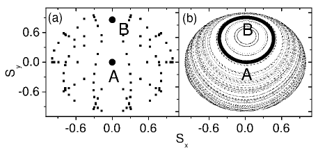
Figure 4: Periodic stroboscopic plots of the projection of spin on the $S_{z}=0$ plane. The thick line and dots correspond to the orbits with initial spin $\vec{S}=\left(0,0,1\right)$. $K=0.8$ (a) $g=0.0$; (b) $g=0.1$.

The motion of the spin is more complicate with interactions. The spin components at $\hat{x}$ and $\hat{y}$ directions can be written as $S_{x}=\sqrt{1-S_{z}^{2}}\cos\alpha$ and $S_{y}=-\sqrt{1-S_{z}^{2}}\sin\alpha$ in terms of population difference $S_{z}$ and relative phase $\alpha$, which yields the relation

$$\dot{S}_{x}=\dot{\alpha}S_{y}-\frac{g}{\pi}S_{z}S_{y}\cos^{2}\alpha$$

during the free evolution. Comparing this equation with the Bloch equation (11), we obtain the equation of motion for the relative phase

$$\dot{\alpha}=\frac{1}{2}+\frac{g}{8\pi}+\frac{g}{2\pi}\left(\cos 2\alpha+\frac{3}{4}\right)S_{z}.$$ (14)

We see the motion between two consecutive kicks is approximately described by a rotation of $\pi+g(1+3S_{z})/4$ about the $z$ axis. Compared with the noninteraction case, the mean field interaction leads to an additional phase shift $g(1+3S_{z})/4$. This phase shift results in a deviation of the spin from $S_{x}=0$ plane at time $2T^{-}$, i.e., moment just before the second kick. As a result, the second kick cannot drive the spin back to its initial position and quantum anti-resonance is absent. However, the phase shift will be accumulated in future evolution and the spin may reach $S_{x}=0$ plane at a certain time $mT^{-}$(beat period) when the total accumulated phase shift is $\pi/2$. Then the next kick will drive spin back north pole by applying an angle $\sqrt{2}K$ rotation about the $x$ axis.

The above picture is confirmed by our numerical solution of the spin Hamiltonian with fourth-order Runge-Kutta method recipe . In Fig. 4, we plot the phase portraits of the spin evolution by choosing different initial conditions of the population difference $S_{z}$ and relative phase $\alpha$. Just after each kick three spin components $S_{i}$ ($i=x,y,z$) are determined and their projections on $S_{z}=0$ plane are plotted. For the noninteraction case (Fig.4(a)), we see the motion of the spin is an osillation between the north pole $A$ and another point $B$, indicating the occurence of quantum anti-resonance. The interaction between atoms changes the phase portraits drametically (Fig.4(b)). Around the north pole, a fixed point surrounded by periodic elliptic orbits appears. The two-point oscillation is shifted slowly and form a continuous and closed orbit, representing the phenomenon of quantum beating.

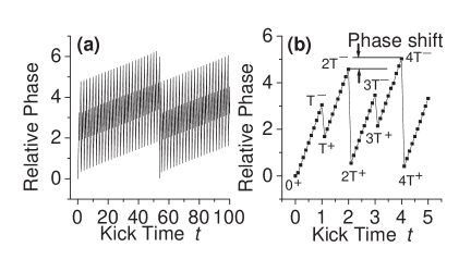
Figure 5: (a) Plots of relative phase versus the number of kicks $t$, where $g=0.1$, $K=0.8$. (b) Schematic plot of the phase shift. $nT^{-(+)}$ represents the moment just before (after) the $n$th kick.

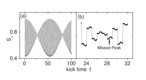
Figure 6: (a) Plot of population difference versus the number of kicks $t$, where $g=0.1$, $K=0.8$. (b) Details of (a) at the middle of a beat period. The population difference decreases in two consecutive kicks.

In Fig.5 we see that the relative phase at the moment just before the even kicks increases almost linearly and reaches $2\pi$ in a beat period. The slope of the increment reads, $\gamma_{RP}=\left(\alpha\left(4T^{-}\right)-\alpha\left(2T^{-}\right)\right)/2$, which can be deduced analytically. With this and through a lengthy deduction, we obtain an analytic expression for the beat frequency to first order in $g$,

$$f_{beat}\approx\frac{g}{4\pi}\left(1+3\cos\left(\sqrt{2}K\right)\right).$$ (15)

In Fig. 6, we plot the evolution of population difference and the phenomenon of quantum beating is clearly seen in the spin model. Notice that there is one peak miss of the oscillation at the middle of one period because the population difference decreases in two consecutive kicks. Taking account of this missed peak, we obtain the oscillation frequency

$$f_{osc}\equiv\frac{N_{total}-N_{miss}}{2N_{total}}=\frac{1}{2}-\frac{1}{2}f_{beat},$$ (16)

where $N_{total}$ and $N_{miss}$ are total and missed numbers of peaks, respectively.

The analytical expressions Eqs. (15) and (16) of the beat and oscillation frequencies are in very good agreement with the numerical results obtained from G-P equation, as shown in Fig.3. Therefore the beating provides a method to measure interaction strength in an experiment.

III.3 Anti-Resonance with interactions

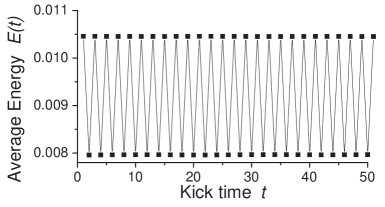
Figure 7: Plots of average energy $E\left(t\right)$ versus the number of kicks $t$ for $K=0.1$, $g=0.1$. $T_{AR}$ is determined through Eq.( 17).

In the spin model, we see that it is the additional phase shift originating from weak interactions that destroys the two kick period recurrence of the anti-resonance and leads to the phenomenon of quantum beating. Therefore we will still be able to observe the quantum anti-resonance even in the presence of interactions if the additional phase shift may be compensated. Actually, the additional phase shift can be cancealed by varying the kick period $T$ so that the relative phase $\alpha$ only change $\pi$ between two consecutive kicks. Using Eq. (14), we find the new kick period for anti-resonance in the presence of interactions may be approximated as

$$T_{AR}\approx\frac{8\pi^{2}}{4\pi+g+3g\cos\left(\sqrt{2}K\right)}$$ (17)

In Fig. 7, we plot the evolution of the average energy $E\left(t\right)$ with the new kick period $T_{AR}$. We see that the energy oscillates between two values and the oscillation period is $2T_{AR}$, clearly indicating the recovery of the anti-resonance.

III.4 Decoherence due to thermal noise

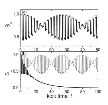
Figure 8: Plots of population difference with respect to the number of kicks in the presence of decoherence. $K=0.8$, $g=0.2$. Thin lines correspond to $\Gamma=0$. Thick lines correspond to (a) $2\pi\Gamma/g=0.001$, (b) $2\pi\Gamma/g=1$.

In realistic experiments, the decoherence effects always exist. Generally, decoherence originates in the coupling to a bath of unobserved degree of freedom, or the interparticle entanglement process decoh . The main source of decoherence in a BEC is the thermal cloud of particles surrounding the condensate. Thermal particles scattering off the condensate will cause phase diffusion at a rate proportional to the thermal cloud temperature. Here we consider a simple model that accounts for the effect of the thermal noise on the two-mode dynamics by adding a $\tau=1/\Gamma$ transversal relaxation term anglin into the mean-field equations of the motion

$$\overset{.}{S}_{x} = \left(\frac{1}{2}+\frac{g}{8\pi}-\frac{g}{8\pi}S_{z}\right)S_{y}-\Gamma S_{x},$$ (18)

$$\overset{.}{S}_{y} = \left(-\frac{1}{2}-\frac{g}{8\pi}-\frac{7g}{8\pi}S_{z}\right)S_{x}-\sqrt{2}KS_{z}\delta_{T}\left(t\right)-\Gamma S_{y},$$

$$\overset{.}{S}_{z} = \frac{g}{\pi}S_{y}S_{x}+\sqrt{2}KS_{y}\delta_{T}\left(t\right).$$

In Fig.8, we plot the evolution of the population difference $S_{z}$ for different decoherence constant $\Gamma$. We see that the phenomenon of quantum beating is destroyed by strong thermal noise (Fig.8(b)), while survives in weak noise (Fig.8(a)). For large decoherence constant, the population difference $S_{z}$ decays to $0$ exponentially and the characteristic time is the just the decoherence time $\tau=1/\Gamma$. Therefore the decoherence time $\tau$ must be much larger than the beat period $2\pi/f_{beat}$ to observe the phenomenon of quantum beating, which yields

$$2\pi\Gamma/g<<\frac{1}{4\pi}(1+3\cos(\sqrt{2}K)).$$ (19)

In the case of $K=0.8$, Eq. (19) gives an estimation $2\pi\Gamma/g<<0.2$, which agrees with the numerical results shown in Fig.8.

IV Strong Interactions: Transition to Instability

IV.1 Characterization of the instability: Bogoliubov excitation

Tuning the interaction strength still larger means enhancing further the nonlinearity of the system. From our general understanding of nonlinear systems, we expect that the solution will be driven towards chaos, in the sense of exponential sensitivity to initial condition and random evolution in the temporal domain. The latter character has been clearly displayed by the irregular pattern of the energy evolution in Fig.1(c). On the other hand, the onset of instability (or chaotic motion) of the condensate is accompanied with the rapid proliferation of thermal particles. Within the formalism of Castin and Dum castin described in Section II, the growth of the number of the noncondensed atom will be exponential, similar to the exponential divergence of nearby trajectories in phase space of classical system. The growth rate of the noncondensed atoms is similar to the Lyapounov exponent, turning from zero to nonzero as instability occurs.

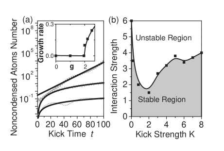
Figure 9: (a) Semilog plot of the mean number of noncondensed atoms versus the number of kicks $t$. The thicker lines are fitting functions. $K=0.8$, $g=0.1$ (dashed line, fitting function $0.0003t^{1.3}$), $g=1.5$ (dotted line, fitting function $0.0011t^{2}$), $g=2.0$ (dash dotted line, fitting function 0.32exp(0.1t)). The inset shows the interaction dependence of the growth rate. The scatters are from numerical simulation and the solid line is the fitting function $0.33{(g-1.96)}^{1/2}$. (b) Phase diagram of the transition to instability.

We numerically integrate Bogoliubov equation (2) for the $u_{k}$, $v_{k}$ pairs over a time span of 100 kicks, using a split operator method, parallel to numerical integration of GP equation (1). The initial conditions

$$\left(\begin{array}[]{c}u_{k}(0)\\ v_{k}(0)\end{array}\right)=\frac{1}{2}\left(\begin{array}[]{c}\zeta+\zeta^{-1}\\ \zeta-\zeta^{-1}\end{array}\right)e^{ik\theta}$$ (20)

for initial ground state wavefunction $\psi(\theta)=1/\sqrt{2\pi}$, are obtained by diagonalizing the linear operator in Eq.(2) castin2 , where $\zeta=\left(\frac{k^{2}/2}{k^{2}/2+2g\left|\psi\right|^{2}}\right)^{1/4}$.

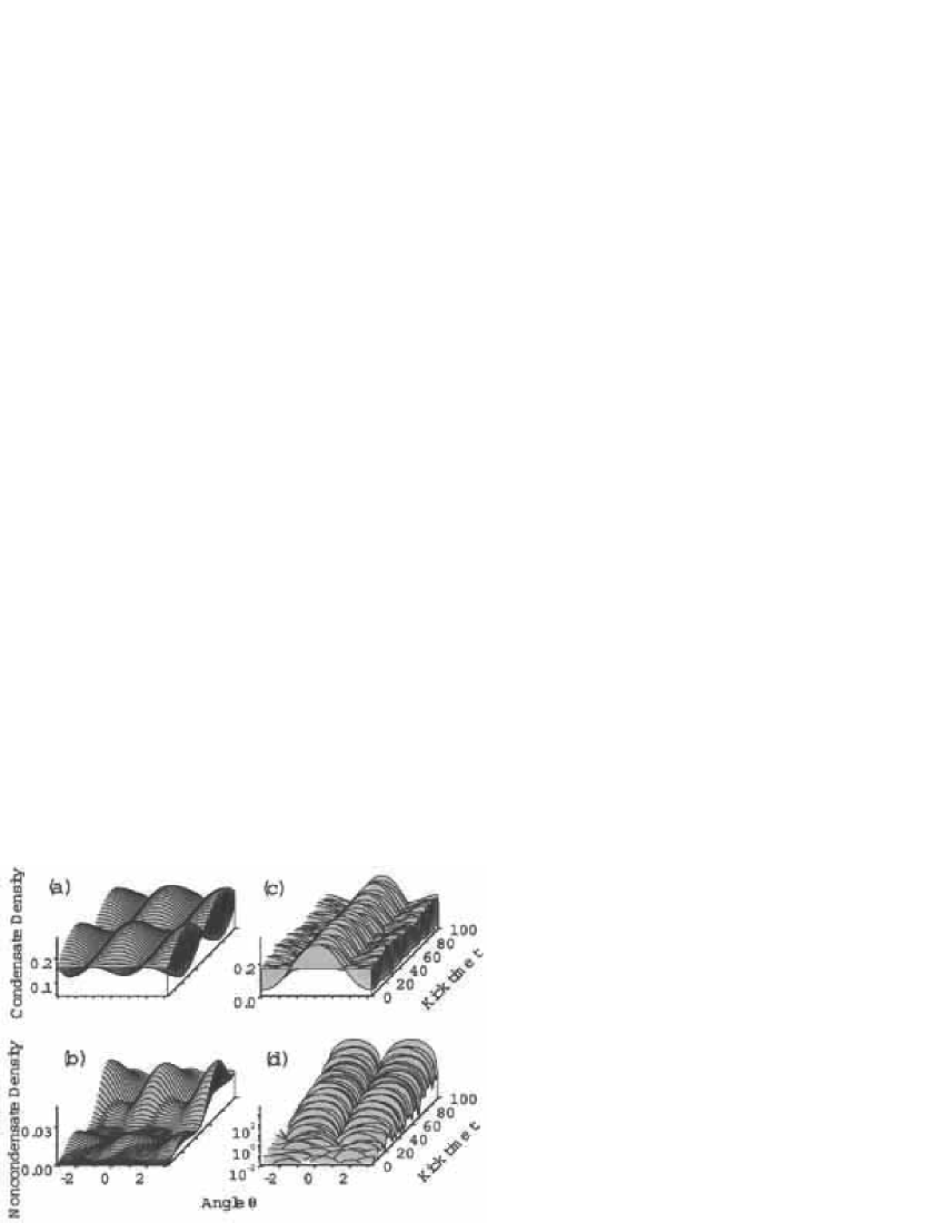
Figure 10: Plots of condensate and noncondensate densities, where $K=0.8$. (a,b) $g=0.1$; (c,d) $g=2.0$.

After each kick the mean number of noncondensed atoms is calculated and plotted versus time in Fig.9(a). We find that there exists a critical value for the interaction strength, i.e., $g_{c}=1.96$, above which, the mean number of noncondensed atoms increases exponentially, indicating the instability of BEC. Below the critical point, the mean number of noncondensed atoms increases polynomially. As the nonlinear parameter crosses over the critical point, the growth rate turns from zero to nonzero, following a square-root law (inset in Fig.9(a)). This scaling law may be universal for Bogoliubov excitation as confirmed by recent experiments ketterle

The critical value of the interaction strength depends on the kick strength. For very small kick strength, the critical interaction is expected to be large, because the ground state of the ring-shape BEC with repulsive interaction is dynamically stable biao . For large kick strength, to induce chaos, the interaction strength must be large enough to compete with the external kick potential. So, in the parameter plane of $(g,k)$, the boundary of instability shows a ”U” type curve (Fig.9(b)).

Across the critical point, the density profiles of both condensed and noncondensed atoms change dramatically. In Fig.10, we plot the temporal evolution of the density distributions of condensed atoms as well as noncondensed atoms. In the stable regime, the condensate density oscillates regularly with time and shows clear beating pattern (Fig.10(a)), whereas the density of the noncondensed atoms grows slowly and shows main peaks around $\theta=\pm\pi$ and $0$, besides some small oscillations (Fig.10(b)). In the unstable regime, the temporal oscillation of the condensate density is irregular (Fig.10(c)), whereas the density of noncondensed atoms grows explosively with the main concentration peaks at $\theta=\pm\pi/2$ where the gradient density of the condensed part is maximum (Fig.10(d)). Moreover, our numerical explorations show that the $\cos^{2}\theta$ mode (Fig10.(b)) dominates the density distribution of the noncondensed atoms as the interaction strength is less than 1.8. Thereafter, the $\sin^{2}\theta$ mode grows while $\cos^{2}\theta$ mode decays, and finally $\sin^{2}\theta$ mode become dominating in the density distribution of noncondensed atoms above the transition point (Fig10.(d)). Since the density distribution can be measured in experiment, this effect can be used to identify the transition to instability.

IV.2 Arnold Diffusion

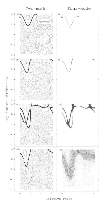
Figure 11: Periodic stroboscopic plots of population difference with respect to the relative phase between the first two modes. $K=0.8$. (a-d) the two-mode model, where (a) $g=0.1$, circle dots corresponds to $g=0$; (b) $g=1.5$; (c) $g=1.9$; (d) $g=2.0$; The thicker line and larger dots on the phase portaits represent the trajectories with initial conditions $S_{z}=1,$ $\alpha=0$. (e-h) the four-mode approximation, the portait is the projection on the first two modes of the trajectory with initial condition $S_{z}=1,$ $\alpha=0$. (e) $g=0.1$; (f) $g=1.6$; (g) $g=2.2$; (h) $g=2.5$.

We have seen that strong interactions destroy beating solution of the GP equation and the motion of the condensate become chaotic, characterized by exponential growth in the number noncondensed atoms. The remaining question is how the motion of condensate is driven to chaos, that is, the route of the transition to instability.

The transition to chaos for the motion of the condensate can be clearly seen in the periodic stroboscopic plots of the trajectories for both two-mode approximation (Fig.11(a-d)) and four-mode approximation (Fig.11(e-f), it is exact for the interaction region we consider in Fig.11) to the original GP equation (1). The solution oscillates between two points $A$ and $B$ (point $C$ is identical to $A$ in spin model.) for noninteraction case, and forms closed path in the phase space for the weak interaction (Fig11.(a)). Note that compared with the two-mode calculation, the effective interaction strength in the four-mode approximation is rescaled, to give the comparable pattern in the phase space.

With increasing interaction strength, the stable quasi-periodic orbits in Fig.11(b) bifurcates into three closed loops (Fig.11(c)) and chaos appears in the neighborhood of the hyperbolic fixed points. However, diffusion from one stochastic region to another are still blocked by KAM tori for the two-mode system. In Fig.11(d), the trajectory with initial condition $S_{z}=1,\alpha=0$ is closer to the chaotic region.

The above discussion is based on two-mode approximation, actually, the solution is coupled with other modes of higher energy states. For small interaction, this coupling is negligible and the four-mode simulation gives the same results as seen in Fig.11(a,b,e,f). For large interaction, this coupling is important and our system is essentially high-dimensional ($d>2$). One important character of a high-dimensional dynamical system is that KAM tori ($d$-dimension) can not seperate phase space ($2d$-dimension) and the whole chaotic region is interconnected. If a trajectory lies in a chaotic region it can circumvent KAM tori and diffuse to higher energy states through Arnold diffusion. This process is clearly demonstrated in Fig.11(g,h). We see that the trajectory diffuses along the separatrix layers, circumvents the KAM tori, and finally spreads over whole phase space (Fig.11(h), $g=2.5$). We also calculate the diffusion coefficient

$$D_{E}=\frac{2}{J(J-1)}\sum_{m>n}\frac{\left|E_{m}-E_{n}\right|^{2}}{T\left(m-n\right)},$$ (21)

where $E_{m}$ is the energy after the mth kick, $J$ is the total number of kicks. For $g=2.2$ and $g=2.5$, the diffusion rates are $7.2\times 10^{-11}$ and $1.5\times 10^{-9}$ respectively.

Arnold diffusion allows the state to diffuse into higher energy states, which destroys quasiperiodic motion of the quantum beating and leads to the transition to instability. As Arnold diffusion occurs, the motion of the condensate becomes unstable and the number of the noncondensed atoms grow exponentially, as we have seen in above discussion.

Arnold diffusion is a general property of the nonlinear Schrödinger equation in the presence of strong interactions. However, it may be hard to observe the whole process of Arnold diffusion in realistic BEC experiments because of the limit number of atoms ($10^{6}$). As Arnold diffusion occurs, the instability of the condensate leads to the exponential growth of thermal atoms which destroy the condensate, as well as invaildate the GP equation (1) in a short time; while clear signature of the whole Arnold diffusion process may only be observed in a realtive long period. On the other hand, Arnold diffusion may be observed in the context of nonlinear optics, where the GP equation (1) describes the propagation of photons. The number of photons is very large and the interactions between them are very weak, therefore it is possible to have a long diffusion process without invalidating the GP equation (1).

IV.3 Dynamical localized states

Although the above discussions have been focused on a periodic state of anti-resonance, the transition to instability due to strong interactions also follows a similar path for a dynamically localized state. The only difference is that we start out with a quasiperiodic rather than periodic motion in the absence of interaction. This means that it will generally be easier to induce instability but still requires a finite strength of interaction.

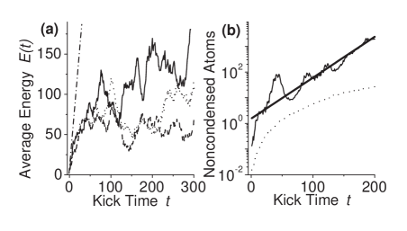
Figure 12: Nonlinear effects on dynamically localized states. $K=5$, $T=1$. (a) Plots of average energy $E(t)$ versus the number of kicks $t$, where dash dotted line corresponds to the classical diffusion. $g=0$ (dash), $g=1$ (dot), $g=5$ (solid). (b) Semilog plot of the mean number of noncondensed atoms versus the number of kicks $t$. $g=1$ (dot), $g=5$ (solid).

In Fig.12, we show the nonlinear effect on a dynamically localized state at $K=5$ and $T=1$. For weak interactions ($g=1$) the motion is quasiperiodic with slow growth in the number of noncondensed atoms. Strong interaction ($g=5$) destroys the quasiperiodic motion and leads to diffusive growth of energy, accompanied with exponential growth of noncondensed atoms that clearly indicates the instability of the BEC. Notice that the rate of growth in energy is much slower than the classical diffusion rate, which means that chaos brought back by interaction in this quantum system is still much weaker than pure classical chaos.

V Conclusions

We have investigated the complex dynamics of a periodically kicked Bose-Einstein condensate that is considered as a nonlinear generalization of the quantum kicked rotor. We demonstrate the transition from the anti-resonance to the quantum beating and then to instability with increasing many-body interactions, and reveal their underlying physical mechanism. The stable quasiperiodic motions for weak interactions, such as anti-resonace and quantum beating, have been studied by mapping the nonlinear Schrödinger equation to a spin model. The transition to instability has been characterized using the growth rate of the noncondensed atoms number, which is polynomial for stable motion and exponential for chaotic motion of the condensate.

Finally, we emphasize that the results obtained in the paper are not limited to BEC and can be directly applied to other systems whose dynamics are governed by the nonlinear Schrödinger equation.

- (1) L. E. Reichl, The Transition to Chaos In Conservative Classical Systems: Quantum Manifestations (Springer-Verlag, New York 1992).
- (2) G. Casati, B. V. Chirikov, J. Ford, and F. M. Izrailev, Lect. Notes Phys. 93, 334 (1979); B. V. Chirikov, Phys. Rep. 52, 263 (1979); F. M. Izrailev, ibid 196, 299 (1990).
- (3) F. M. Izrailev, and D. L. Shepelyansky, Sov. Phys. Dokl. 24, 996 (1979); Theor. Math. Phys. 43, 553 (1980); I. Dana, E. Eisenberg, and N. Shnerb Phys. Rev. Lett. 74, 686 (1995).
- (4) F. L. Moore, J. C. Robinson, C. F. Bharucha, Bala Sundaram, and M. G. Raizen, Phys. Rev. Lett. 75, 4598 (1995); W. H. Oskay, D. A. Steck, V. Milner, B. G. Klappauf, and M. G. Raizen. Opt. Comm. 179, 137 (2000); M. B. d’Arcy, R. M. Godun, M. K. Oberthaler, D. Cassettari, and G. S. Summy, Phys. Rev. Lett. 87, 074102 (2001).
- (5) F. Benvenuto, G. Casati, A. Pikovsky, and D. L. Shepelyansky, Phys. Rev. A 44, R3423 (1990); D. L. Shepelyansky, Phys. Rev. Lett. 70, 1787 (1993).
- (6) S. A. Gardiner, D. Jaksch, R. Dum, J. I. Cirac, and P. Zoller, Phys. Rev. A 62, 023612 (2000); R. Artuso and L. Rebuzzini, Phys. Rev. E 66, 017203 (2002).
- (7) M. H. Anderson, J. R. Ensher, M. R. Matthews, C. E. Wieman, and E. A. Cornell, Science 269, 198 (1995); C. C. Bradley, C. A. Sackett, J. J. Tollet, and R. Hulet, Phys. Rev. Lett. 75, 1687 (1995); K. D. Davis, M.-O. Mewes, M. R. Andrews, N. J. van Druten, D. S. Durfee, D. M. Kurn, and W. Ketterle, ibid 75, 3669 (1995);
- (8) F. Dalfovo, S. Giorgini, L. P. Pitaevskii, and S. Stringari, Rev. Mod. Phys. 71, 463 (1999); A. J. Leggett, ibid 73, 307 (1999);
- (9) R. W. Boyd, Nonlinear Optics (Academic Press, San Diego 1992).
- (10) A. Vardi and J.R. Anglin, Phys. Rev. Lett. 86, 568 (2001); G.P. Berman, A. Smerzi, and A. R. Bishop, ibid 88, 120402 (2002).
- (11) Y. Castin and R. Dum, Phys. Rev. A 57, 3008 (1998); Phys. Rev. Lett. 79, 3553 (1997); Ph. Nozières and D. Pines, The Theory of Quantum Liquids, Vol. II. (Addison-Wesley Reading, MA 1990).
- (12) J. K. Chin, J. M. Vogels, and W. Ketterle, Phys. Rev. Lett. 90, 160405 (2003).
- (13) C. Zhang, J. Liu, M. G. Raizen, and Q. Niu Phys. Rev. Lett. 92, 054101 (2004).
- (14) B. Hu, B. Li, J. Liu and J. Zhou, Phys. Rev. E 58, 1743 (1998); B. Hu, B. Li, J. Liu, and Y. Gu, Phys. Rev. Lett. 82, 4224 (1999).
- (15) V. I. Arnol’d, Sov. Math. Doklady 5, 581 (1964); K. Kaneko, and R. J. Bagley, Phys. Lett. A 110, 435 (1985); A. J. Lichtenberg and B. P. Wood, Phys. Rev. A 39, 2153 (1989); B. P. Wood, A. J. Lichtenberg, and M. A. Lieberman, ibid 42, 5885 (1990); D. M. Leitner, and P. G. Wolynes, Phys. Rev. Lett. 79, 55 (1997); V. Ya. Demikhovskii, F. M. Izrailev, and A. I. Malyshev, ibid 88, 154101 (2002);
- (16) T. Hogg and B.A. Huberman, Phys. Rev. Lett. 48, 711 (1982); S. Fishman, D.R. Grempel, and R.E. Prange, ibid 49, 509 (1982).
- (17) L.D. Carr, C.W. Clark, and W.P. Reinhardt, Phys. Rev. A 62, 063610 (2000); G.M. Kavoulakis, ibid 67, 011601 (2003); R. Kanamoto, H. Saito, and M. Ueda, ibid 67, 013608 (2003).
- (18) V. Milner, J.L. Hanssen, W.C. Campbell, and M.G. Raizen, Phys. Rev. Lett. 86, 1514 (2001); N. Friedman, A. Kaplan, D. Carasso, and N. Davidson, ibid 86, 1518 (2001).
- (19) E. M. Wright, J. Arlt, and K. Dholakia, Phys. Rev. A 63, 013608 (2000).
- (20) B. Mieck, and R. Graham, arXiv.org:cond-mat/0411648.
- (21) J.M. Gerton, D. Strekalov, I. Prodan, R.G. Hulet, Nature 408, 692 (2000); E.A. Donley, N.R. Claussen, S.L. Cornish, J.L. Roberts, E.A. Cornell, C.E. Wieman, ibid 412, 295 (2001).
- (22) A.D. Bandrauk, and H. Shen, J. Phys. A 27, 7147 (1994).
- (23) Jie Liu, Biao Wu, and Qian Niu Phys. Rev. Lett. 90, 170404 (2003);
- (24) F. Haake, Quantum Signature of Chaos (Springer-Verlag, New York 2000).
- (25) W.H. Press, et al., Numerical Recipes in C++ (Cambridge, New York 2000).
- (26) J. R. Anglin and A. Vardi, Phys. Rev. A 64, 013605 (2001).
- (27) W. H. Zurek, Rev. Mod. Phys. 75, 715 (2003).
- (28) Y. Castin, in Coherent Atomic Matter Waves, edited by R. Kaiser, et al., (EDP Sciences and Springer-Verlag 2001).
- (29) B. Wu and Q. Niu, Phys. Rev. A 64, 061603 (2001); J.R. Anglin, ibid 67, R051601 (2003).