Kuramoto Oscillators on Chains, Rings and Cayley-trees

Abstract

We study systems of Kuramoto oscillators, driven by one pacemaker, on $d$-dimensional regular topologies like linear chains, rings, hypercubic lattices and Cayley-trees. For the special cases of next-neighbor and infinite-range interactions , we derive the analytical expressions for the common frequency in the case of phase-locked motion and for the critical frequency of the pacemaker, placed at an arbitrary position on the lattice, so that above the critical frequency no phase-locked motion is possible. These expressions depend on the number of oscillators, the type of coupling, the coupling strength, and the range of interactions. In particular we show that the mere change in topology from an open chain with free boundary conditions to a ring induces synchronization for a certain range of pacemaker frequencies and couplings, keeping the other parameters fixed. We also study numerically the phase evolution above the critical eigenfrequency of the pacemaker for arbitrary interaction ranges and find some interesting remnants to phase-locked motion below the critical frequency.

I Introduction

Synchronization is an ubiquitous phenomenon, found in a variety of natural systems like fireflies, where the males flash light in synchrony to attract the females fireflies , chirping crickets crickets , or like neural systems, but also utilized for artificial systems of information science in order to enable a well-coordinated behavior in time. As an important special case, the coordinated behavior refers to similar or even identical units like oscillators that are individually characterized by their phases and amplitudes. A further reduction in the description was proposed by Kuramoto for an ensemble of $N$ oscillators kuraoriginal , after Winfree had started with a first model of coupled oscillators winfree . Within a perturbative approach Kuramoto showed that for any system of weakly coupled and nearly identical limit-cycle oscillators, the long-term dynamics is described by differential equations just for the phases $\varphi_{i}$ (not for the amplitudes) with mutual interactions, depending on the phase differences in a bounded form. Kuramoto solved this model for the special case of all-to-all coupled oscillators, for identical interaction functions, and for eigenfrequencies, taken out of a narrow distribution. It is, however, this model, later named after him, that nowadays plays the role of a paradigm for weakly and continuously interacting oscillators. In a large number of succeeding publications the original Kuramoto model was generalized in various directions, for a recent review see kuramotoreview . In particular the eigenfrequencies were specialized in a way that one oscillator plays the role of a pacemaker with eigenfrequency different from zero, while all others have eigenfrequency zero yamada . In yamada the pacemaker was placed at a specific position, the beginning of a linear chain. Moreover the interaction range was changed from all-to-all to next neighbor interactions daido strogatz . In daido the system was studied numerically, and an abrupt change from long-to short-term interaction was suggested.
In this paper we consider a system of Kuramoto oscillators, coupled on various regular lattice topologies, and driven by a pacemaker, placed at an arbitrary site of the lattice. The interaction range is neither restricted to next-neighbor nor to all-to-all couplings, but varied by a parameter $\alpha$ that tunes the decay with the distance between the interacting units. We analytically derive the common frequency $\Omega$ of phase-locked motion and the upper bound on the absolute value of the ratio of the pacemaker’s frequency to the coupling strength $\left|\omega_{s}/K\right|$ for next-neighbor and all-to-all couplings in case of $d$-dimensional regular lattices with open or closed boundaries, in particular for a ring and an open chain. The results show the dependence on the size of the system (total number $N$ of oscillators), the position $s$ of the pacemaker (for open boundary conditions) and the (a)symmetric treatment of the pacemaker’s interaction with the other Kuramoto oscillators (tuned by the parameter $\epsilon_{s}$). The intermediate interaction range $(0<\alpha<\infty)$ as well as the phase evolution in the desynchronized phase (above the threshold for phase-locked motion) are treated numerically.

The paper is organized as follows. In section II we define the model and identify the various special cases. Section III is devoted to the study of phase-locked motion. We calculate the common frequency and the critical threshold for phase-locked motion for a linear chain and $\alpha\to\infty$ (section III.1), for a ring and $\alpha\to\infty$ in section III.2, the case of all-to-all couplings ($\alpha=0$) in section III.3. Our main result about a switch to synchronization via the closure of a chain is stated in section III.4. Section III.5 presents our results of numerical simulations for the intermediate interaction range ($0<\alpha<\infty$). In section III.6 we generalize the previous results to regular lattice topologies in higher dimensions, i.e. to Cayley-trees and d-dimensional hypercubic lattices). In section IV we report on numerical results for the phase portrait above the critical threshold, in the desynchronized phase, in which the phases appear as a superposition of a fast motion, determined by the pacemaker, and a slow motion, determined by the interaction of all other oscillators. Finally we give the summary and conclusions in section V. Details of the analytical calculations are postponed to the Appendix.

II The Model

The system is defined on a $d$-dimensional lattice, where each site is a limit-cycle oscillator. The phase of the $i$-th oscillator obeys the dynamics determined by

$$\dot{\varphi}_{i}=\delta_{i,s}\omega_{s}+(1+\delta_{i,s}\epsilon_{s})\ \frac{K}{\eta_{i}}\ \sum_{j\neq i}\frac{\sin{(\varphi_{j}-\varphi_{i})}}{r_{ji}^{\alpha}}\;\;\;,\;\forall\;i=0,\ldots,N\;\;\;,$$ (1)

where

$$\eta_{i}:=\sum_{j\neq i}r^{-\alpha}_{ji}\;\;\;,\;\forall\;i=0,\ldots,N\;\;\;.$$ (2)

In particular $\varphi_{i}$ is the phase of the i-th oscillator, the index $s$ labels the pacemaker with eigenfrequency $\omega_{s}\neq 0$, while all other oscillators have eigenfrequency zero. The parameter $-1\leq\epsilon_{s}\leq 0$ serves to tune the interaction of the pacemaker with the other oscillators. For $\epsilon_{s}=0$ the pacemaker is on the same footing as the other oscillators, being only distinct by its eigenfrequency $\omega_{s}$. For $\epsilon_{s}=-1$ its interaction is asymmetric in the sense that the pacemaker influences the other oscillators, but not vice versa (the pacemaker acts as an external force), so that it is on a different level in the hierarchy of the system. (In natural systems both extreme cases as well as intermediate couplings may be realized: a pacemaker being one out of an ensemble of oscillators or being distinct by additional features to the eigenfrequency.) The constant $K>0$ parameterizes the coupling strength, $\eta_{i}$ represents a space-dependent normalization, it replaces the factor $N$ that is used for all-to-all interactions and turns out to be essential for the $\alpha$-dependence of the synchronization threshold, cf. section III.5. The phases of the i-th and j-th oscillators interact via the sine function (as originally proposed by Kuramoto), of which two properties enter the analytical predictions: the sine is bounded and an odd function. The distance $r_{ij}$, given in units of the edges of the lattice, enters to the power $-\alpha$, $\alpha=0$ gives the space-independent all-to-all coupling, originally considered by Kuramoto, $\alpha\to\infty$ is understood to restrict the interactions to nearest neighbors. The label of the oscillator simultaneously specifies the location in space, see e.g. Figure 1 for a one-dimensional chain, where coordinate $s$ specifies the position of the pacemaker.

Figure 1: One-dimensional lattice with $\left(N+1\right)$ Kuramoto oscillators, labelled by their coordinates.

System (1) contains the original model of Kuramoto as special case for $\epsilon_{s}=0$, $\alpha=0$ and absent $\delta_{i,s}$ (all oscillators with an eigenfrequency chosen at random from a probability distribution). Note that the interaction strength is symmetric between oscillators $i,j$, with $i,j\neq s$, continuous in time and instantaneous. It depends on the natural or artificial systems that are modelled by Kuramoto oscillators, whether these features amount to appropriate idealizations or to an oversimplification. For example, the interactions between fireflies propagate with the very velocity of light. In view of their mutual distances on the trees the delay caused by the finite velocity of light should be completely negligible. When the interaction proceeds via pulses as in neural systems, the continuous interaction [as in system (1)] is also not adequate.

III Phase-locked Motion

In this section we consider the conditions for having phase-locked motion, in which the phase differences between any pair of oscillators remain constant over time, after an initial relaxation time. In general two quantities are of interest for phase-locked motion, the frequency $\Omega$, in common to all oscillators in the phase-locked state, and the critical threshold in terms of the absolute value of the eigenfrequency of the pacemaker $\left|\omega_{s}\right|$ over the coupling strength $K$, i.e. $\left|\omega_{s}/K\right|_{C}$, that gives an upper bound for having phase-locked motion as a stable state. We analytically calculate (see the Appendix) $\Omega$ for any dimension $d$ of the lattice and for arbitrary range of the interaction (i.e. $0\leq\alpha\leq\infty$). Imposing the phase-locked condition

$$\dot{\varphi}_{i}\equiv\Omega\;\;\;,\;\forall\;i=0,\ldots,N$$

to system (1) and using the fact that the sine is an odd function, one easily obtains

$$\Omega\;=\;\frac{N\eta_{s}\omega_{s}}{(1+N\epsilon_{s})\sum_{i\neq s}\eta_{i}+\sum_{j\neq s}\sum_{i\neq j}\eta_{i}}\;\;,$$ (3)

where the $\eta_{i}$s are defined in Eq.(2). They contain the informations about the range of the interactions and about the topology on which the system is defined (i.e. $\eta_{i}$ is a function of $\alpha$, it depends on the dimension $d$ and on the boundary conditions of the lattice). Moreover, in case of periodic boundary conditions and in case of long-range interactions ($\alpha=0$), we find

$$\eta_{i}\equiv\eta\;\;\;,\;\forall\;i=0,\ldots,N\;\;\;,$$

or, in other words, the normalization factor defined in Eq.(2) becomes independent on $i$ (i.e. the position on the lattice of the $i$-th oscillator). In this case we are able to prove that Eq.(3) takes the explicit form

$$\Omega=\frac{\omega}{N+\epsilon N+1}\;\;\;.$$ (4)

The main result is that Eq.(4) is independent on $\alpha$. Moreover, in such cases the position of the pacemaker does not change the behavior of the system. Therefore we dropped the index $s$ of the pacemaker in Eq.(4) .
As a next step, we calculate the critical threshold $\left|\omega_{s}/K\right|_{C}$ for a one-dimensional lattice and different range of interactions: analytically for next-neighbor $(\alpha\to\infty)$ and for long-range $(\alpha=0)$ interactions (section III.1-III.3), numerically for intermediate coupling range (section III.5). Both quantities, the common frequency $\Omega$ and the critical threshold $\left|\omega_{s}/K\right|_{C}$, have an analytical generalization to higher dimensions $d>1$ (section III.6).
All numerical results (apart from those of Figure 9) are obtained with an accuracy of $5\cdot 10^{-6}$ by integrating the system (1) by the fourth-order Runge-Kutta method (with fixed time step $\Delta t=0.05$).

III.1 Kuramoto oscillators on a linear chain with next-neighbor interactions

We consider $(N+1)$ Kuramoto oscillators coupled along a chain as indicated in Figure 1 with free boundary conditions at the positions $0$ and $N$, and the pacemaker located at position $s$, $0\leq s\leq N$. For this simple topology, Eq.(2) takes the form

$$\eta_{i}=\theta(i)\sum_{j=1}^{i}j^{-\alpha}\;+\;\theta(N-i)\sum_{j=1}^{N-i}j^{-\alpha}\;,\forall i=0,\ldots,N\;,$$ (5)

where $\theta(x)$ is the Heaviside step function [$\theta(x)=1$ for $x>0$ and $\theta(x)=0$ for $x\leq 0$]. Eq.(5) inserted into Eq.(3) gives the proper value of the common frequency $\Omega$ as function of the position $s$ and the eigenfrequency $\omega_{s}$ of the pacemaker, the size of the system $N$ as well as the range of the interaction, parameterized by $\alpha$.
To derive the critical frequency of the pacemaker in the case of next-neighbor interactions $(\alpha\to\infty)$, we use the odd parity of the sine function. We derive a recursive relation between the phase differences of next-neighbor oscillators. Using the boundary conditions it is possible to express these recursive equations in terms of $s$, $N$, $\Omega$, and $K$. On the other hand, the sine function is bounded. These bounds induce the bound on the maximal pacemaker frequency $\left|\omega_{s}/K\right|_{C}$ that is compatible with a phase-locked motion. During the recursions between phase differences we have to distinguish whether we move to the boundary to the right or to the left of the pacemaker $s$, placed between $0<s<N$; either the boundary conditions enter for oscillator $N$ or oscillator $0$. Thus if we move to the right, we obtain for the maximal pacemaker’s frequency

$${}^{R}\left|\frac{\omega_{s}}{K}\right|_{C}=\frac{(N-1)(1+\epsilon_{s})+1}{2N-2s-1}\;,$$ (6)

so that all oscillators to the right ($R$) of $s$ approach a phase-locked state, and

$${}^{L}\left|\frac{\omega_{s}}{K}\right|_{C}=\frac{(N-1)(1+\epsilon_{s})+1}{2s-1}$$ (7)

as bound for oscillators on the left ($L$) of $s$ to synchronize in a phase-locked motion. Since we are interested in a state with all oscillators of the chain being phase-entrained, we need the stronger condition given by

$$\left|\frac{\omega_{s}}{K}\right|_{C}=\min{\left[\;{}^{R}\left|\frac{\omega_{s}}{K}\right|_{C}\;,\;^{L}\left|\frac{\omega_{s}}{K}\right|_{C}\;\right]}\;\;.$$ (8)

For the pacemaker placed at the boundaries $s=N$ or $s=0$ we have

$$\left|\frac{\omega_{s}}{K}\right|_{C}=\frac{2N+2N\epsilon_{s}-\epsilon_{s}}{2N-1}\;\;.$$ (9)

If the pacemaker is located in the middle of the chain, i.e. at $s=N/2$ for $N$ even or $s=(N\pm 1)/2$ for $N$ odd, we have

$$\left|\frac{\omega_{N/2}}{K}\right|_{C}=\frac{(N-1)(1+\epsilon_{N/2})+1}{N-1}\textrm{ , if }N\textrm{ is even}$$ (10)

and

$$\left|\frac{\omega_{(N\pm 1)/2}}{K}\right|_{C}=\frac{(N-1)(1+\epsilon_{(N\pm 1)/2})+1}{N}\textrm{ , if }N\textrm{ is odd}\;.$$ (11)

Note that for $\epsilon_{s}=-1$ the critical ratio goes to zero for $N\to\infty$, while it approaches one for $\epsilon_{s}=0$ and $N\to\infty$, but the common frequency $\Omega$ goes to zero in this case for $N\to\infty$. Moreover we see the stronger the coupling $K$, the larger $\left|\omega_{s}\right|$ may be up to which the system is able to follow the pacemaker.

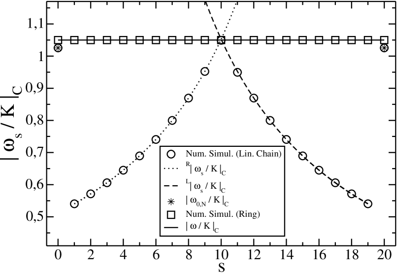
Figure 2: Critical threshold $\left|\omega_{s}/K\right|_{C}$ as function of the position $s$ of the pacemaker on a one-dimensional lattice (for both free and periodic boundary conditions). Here $N=20$, $\alpha=100.0$ and $\epsilon_{s}=0$. Theoretical predictions [dotted, dashed and full lines from Eq.s(6), (7) and (14),respectively, and stars from Eq.(9)] are in perfect agreement with results obtain from numerical simulations (circles and squares).

III.2 Ring topology and next-neighbor interactions

For $\alpha\to\infty$ and $(N+1)$ oscillators placed on a ring, it is easy to see that the normalization factor defined in Eq.(2) is the same for all oscillators $i$ [therefore Eq.(4) gives the right value of $\Omega$]. It can be written as

$$\eta=\left\{\begin{array}[]{ll}2\sum_{j=1}^{N/2}\;j^{-\alpha}&\textrm{ , if }N\textrm{ is even}\\ 2\sum_{j=1}^{(N-1)/2}\;j^{-\alpha}\;+\;\left(\frac{N+1}{2}\right)^{-\alpha}&\textrm{ , if }N\textrm{ is odd}\end{array}\right.\;\;\;.$$ (12)

The derivation on the upper bound of the pacemaker’s frequency $\left|\omega/K\right|_{C}$ for a ring proceeds in analogy to Eq.s (6), (7) and (9), apart from the fact that the boundary conditions are periodic

$$\varphi_{t}\equiv\varphi_{\left(N+1\right)+t}\;\;\;,\;t\in\mathbb{Z}\;.$$ (13)

The result is

$$\left|\frac{\omega}{K}\right|_{C}\;=\;\frac{N+N\epsilon+1}{N}\;\;\;.$$ (14)

III.3 All-to-all coupling

In case of all-to-all coupling ($\alpha=0$) the topology of the system has no longer an effect on the phase entrainment; moreover the normalization factor of definition (2) is $\eta_{i}\equiv N\;\;,\;\forall\;i=0,\ldots,N$, therefore the common frequency is given by Eq.(4). Since we know that in the case of all-to-all couplings the mean-field approximation becomes exact, it is natural to introduce a quantity that usually serves as order parameter kuraoriginal for indicating the synchronized phase, i.e.

$$R\;e^{i\psi}:=\frac{1}{N}\sum_{j\neq s}e^{i\varphi_{j}}\;\;\;.$$ (15)

In our definition $R\;e^{i\psi}$ differs from the usual order parameter only by the fact that the sum runs over $j\neq s$. In terms of the order parameter we can rewrite the system (1) according to

$$\left\{\begin{array}[]{ll}\Omega=\omega_{s}+(1+\epsilon_{s})KR\sin{(\psi-\varphi_{s})}&\\ \Omega=\frac{K}{N}\sin{(\varphi_{s}-\varphi_{i})}+KR\sin{(\psi-\varphi_{i})}&\textrm{ , }\forall\;i\neq s\end{array}\right.\;.$$ (16)

As we see from Eq.s (16), all oscillators different from the pacemaker satisfy exactly the same equation. One possible solution is given by

$$\varphi_{i}\equiv\psi\;\textrm{ , }\forall\;i\neq s\;\;\;,$$

so that all phases of the oscillators different from the pacemaker are equal. Using system (16) and the fact that the sine function is bounded, it is easily seen that the critical ratio $\left|\omega/K\right|_{C}$ is still given by Eq.(14), valid for the ring and $\alpha\to\infty$.

III.4 A switch to synchronization

Let us summarize the results we obtained so far in Figure 2. The full lines represent the analytical results for $\left|\omega_{s}/K\right|_{C}$ for the open chain with $\alpha\to\infty$, more precisely for $\alpha=100$, and the ring for $\alpha=100$, the circles and squares represent numerical data that reproduce the analytical predictions within the numerical accuracy. All results are obtained for $N=20$ and $\epsilon_{s}=0$, they are plotted as a function of the pacemaker’s position that only matters in case of the open chain and for $\alpha>0$. The horizontal line at $\left|\omega_{s}/K\right|_{C}=(N+1)/N$ obviously refers to the ring, the two branches (left and right), obtained for the chain, cross this line when the pacemaker is placed at $s=N/2$ in the middle of the chain. When the pacemaker is located at the boundaries $s=0$ and $s=N$, we obtain two isolated data points, cf. the corresponding Eq.(9), close to the horizontal line.
Let us imagine that for given $N$ and $\epsilon_{s}$ the absolute value of the pacemaker’s frequency $\left|\omega_{s}\right|$ and the coupling $K$ are specified out of a range for which

$$\left|\frac{\omega_{s}}{K}\right|_{C}\;<\;\left|\frac{\omega_{s}}{K}\right|\;\leq\;\left|\frac{\omega}{K}\right|_{C}$$

such that the ratio is too large to allow for phase-locked motion on a chain, but small enough to allow the phase-entrainment on a ring. It is then the mere closure of the open chain to a ring that leads from non-synchronized to synchronized oscillators with phase-locked motion. Therefore, for a whole range of ratios $\left|\omega_{s}/K\right|$, no fine-tuning is needed to switch to a synchronized state, but just a simple change in topology. Because of its simplicity we suspect that this mechanism is realized in biological systems that need the possibility of an easy switch between synchronization and desynchronization. In our numerical integration we simulated such a switch and plot the phase portrait in Figure 3. The phase evolution $\varphi$ as function of time is always projected to the interval $\left[0,2\pi\right)$: we use a thick black line for the phase of the pacemaker and thin dark-grey lines for the other oscillators. In the numerical simulation with $T=8000$ integration steps over time we analyzed a one-dimensional lattice of Kuramoto oscillators with $N=6$, $\alpha=5.0$, $s=2$, $\omega_{s}/K=1$ and $\epsilon_{s}=0$. In the time interval from $0$ to “ON” ($T/3$) we see for the system motions with non-constant slopes: more steep for the pacemaker and the left part of the system (oscillators $i=0,1$) and less steep for the right part (oscillators $i=3,4,5,6$). At the instant “ON” we close the chain, passing to a ring topology. The system almost instantaneously reaches a phase-locked motion (all phases moving with the same slope). At time “OFF” ($2T/3$) we open the ring, again, and the system shows qualitatively the same behavior as before the closure.

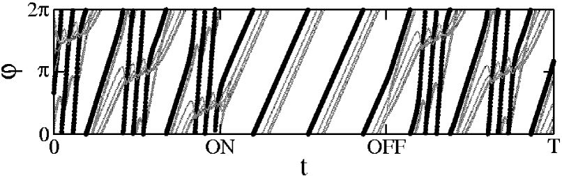
Figure 3: Phase portrait of a system of Kuramoto oscillators on a one-dimensional lattice with $N=6$, $\alpha=5$, $s=2$, $\epsilon_{s}=0$ and $\omega_{s}/K=1$. The phase of the pacemaker is represented by the fat black line, while the phases of the other oscillators are drawn with thin dark-grey lines. We start from a chain (free boundary conditions), for which we are above the critical threshold given in Eq.(8), here the stable state of the system is characterized by a non-constant frequency (the frequency of the oscillators are different from each other and vary during time). We observed the system for $8000$ integration steps altogether. At the instant “ON” ($T/3$) we closed the chain, passing to a ring topology: now the ratio $\omega/K$ is less than the one given by Eq.(14), so that the system can synchronize in the frequency domain (it reaches a phase-locked motion where all the phases have the same constant slope). At instant “OFF” ($2T/3$) we opened the ring and the system falls again into a non-phase-locked motion, similarly to that seen in the interval [$0$,ON].

Furthermore it should be noticed from Figure 2 that it is also favorable to put the pacemaker at the boundaries of an open chain to facilitate synchronization. For $d=1$ the pacemaker then has to entrain only one rather than two nearest neighbors so that the range of allowed frequencies $\left|\omega_{s}\right|$ increases.
¿From these results it is natural to try to utilize the topology in a way that facilitates synchronization in artificial networks when synchronized states are needed. Given $N$ oscillators and a number of $p_{0}$ pacemakers, one can optimize the placement of the pacemakers when only a limited range of couplings is available and no other fine-tuning of parameters is feasible.

III.5 Intermediate range of couplings

Recall from section III that the common frequency $\Omega$ of phase-locked motion was independent on $\alpha$ in case of a ring and depending on $\alpha$ in a well-defined way [cf. Eq.s(3),(5)] in case of an open chain. The upper bound on the pacemaker’s frequency, however, was analytically derived only for $\alpha=0$ and $\alpha\to\infty$. For intermediate values of $\alpha$ we studied the behavior of $\left|\omega_{s}/K\right|_{C}$ as a function of $\alpha$ numerically. The results are shown in Figures 4 and 5.

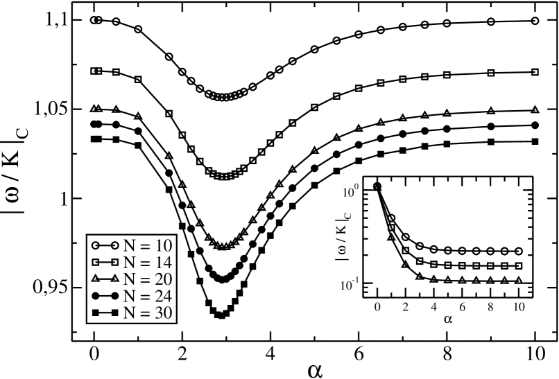
Figure 4: Critical ratio $\left|\omega/K\right|_{C}$ for a one-dimensional ring with $\epsilon=0$ as function of $\alpha$ for various system sizes, showing a non-monotonic behavior with a minimum at $\alpha_{M}\leq 3$. The inset shows the same critical ratio for $N=10,14,20$, but for the system (1) with $\eta=N$, chosen independently on $\alpha$: now $\left|\omega/K\right|_{C}$ behaves as a monotonically decreasing function of $\alpha$.

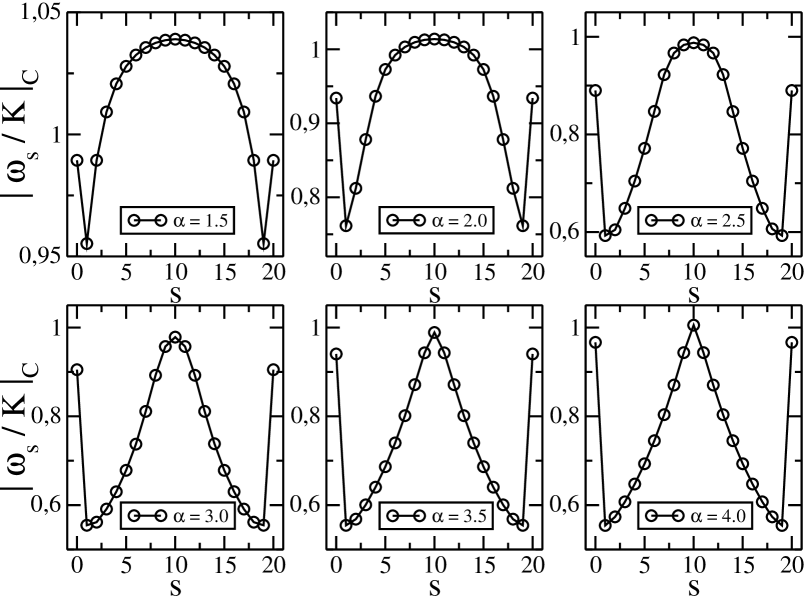
Figure 5: Critical ratio $\left|\omega_{s}/K\right|_{C}$ as function of the pacemaker’s position for an open chain and various values of $\alpha$, indicating a qualitative change in the behaviour between $\alpha=2.5$ and $\alpha=3$.

In case of the ring topology (Figure 4) we observe a non-monotonic function of $\alpha$ with a minimum at $\alpha_{M}\leq 3$ that seems to decrease as the system size increases, here from $N=10$ to $30$. The shape of $\left|\omega_{s}/K\right|_{C}$ depends on the choice of the normalization with $K/\eta_{i}$ in the interaction term of Eq.(1). If we had chosen $K/N$ instead of $K/\eta_{i}$, we would find a monotonic decrease (inset of Figure 4). Instead we see here that all-to-all and next-neighbor interactions lead to the same ratio of $\left|\omega/K\right|_{C}$, while synchronization becomes more and more difficult for $\alpha$ around $\alpha_{M}$. The existence of $\alpha_{M}$ is also supported by numerical results of rogers for $N=100$ oscillators, where it was found that the system approaches the same behavior as the original Kuramoto model with $\alpha=0$ for $\alpha\leq 2$ so that there is a different behavior for long- and intermediate-range couplings. We expect that our values for $\alpha_{M}$ decrease to $\alpha_{M}\propto 2$ for larger system sizes.
Figure 5 shows the same critical ratio $\left|\omega_{s}/K\right|_{C}$ as a function of the pacemaker’s position $s$ for an open chain, $N=20$, $\epsilon_{s}=0$, and various values of $\alpha$. Here it is interesting to see that the shape of $\left|\omega_{S}/K\right|_{C}$ drastically changes around the same value of $\alpha_{M}\leq 3$ as for the ring: for $\alpha<\alpha_{M}$, the critical fraction looks differentiable for all positions $s$ of the pacemaker along the chain, apart from the boundaries $s=0$ and $s=N$, while for $\alpha>\alpha_{M}$ it appears non-differentiable around $s=N/2$ and has a cusp. An analytical understanding of $\left|\omega_{S}/K\right|_{C}$ as a function of $s$ and $\alpha$ is still missing.

III.6 Kuramoto oscillators on regular structures in higher dimensions

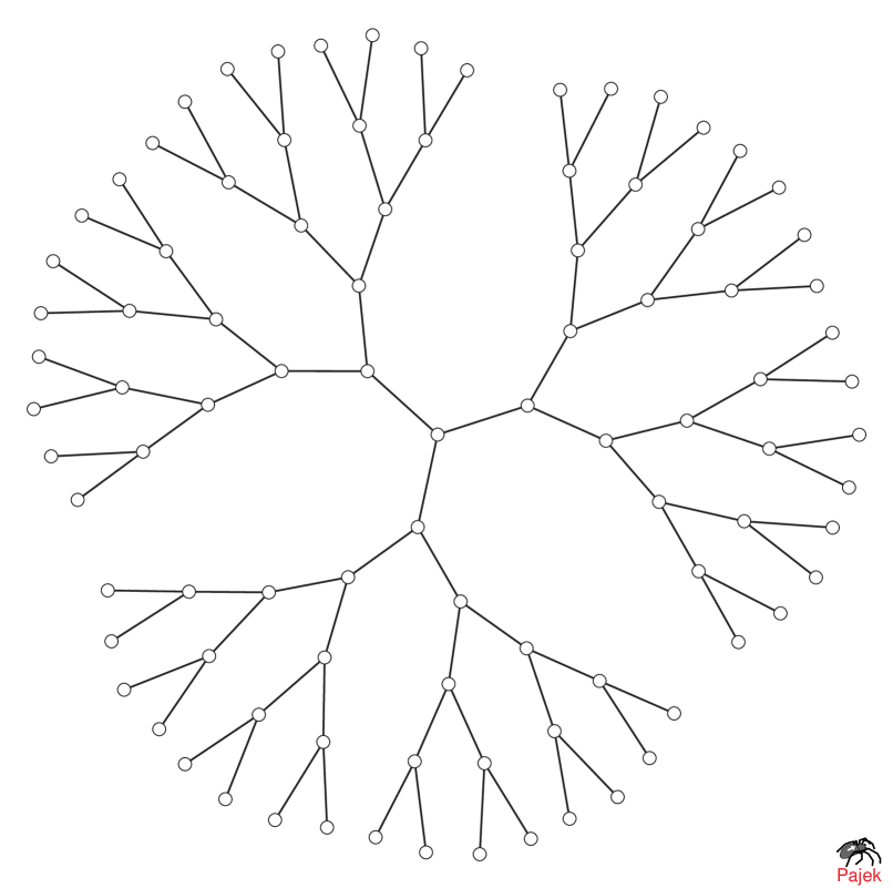
Figure 6: A Cayley tree with $z=3$ branches and radius $R=5$.

In order to generalize our previous results to regular structures in higher dimensions, we consider Cayley-trees and hypercubic lattices. Cayley-trees have $z$ branches to nearest neighbors at each node, cf. Figure 6, apart from nodes in the outermost shell, where the number of nearest neighbors is only $z-1$. Cayley-trees generalize linear chains from $z=2$ to $z>2$ branchings at each node. They provide a geometry that often allows for exact analytical solutions, cf. the percolation problem on a Cayley-tree havlin . Cayley-trees are infinite-dimensional in the sense that the number of nodes in the boundary (outermost shell at distance $R$ from the origin) are proportional to the volume, i.e. the total number of nodes in the tree. Throughout our calculations we place one pacemaker in the center of the tree and assign all other Kuramoto oscillators with eigenfrequency zero to the remaining nodes. We start from a modified version of the equations (1)

$$\dot{\varphi}_{i}=\delta_{i,0}\omega_{0}+\frac{K}{z}\ \sum_{j\neq i}A_{ji}\;\sin{(\varphi_{j}-\varphi_{i})}\;\;\;,\;\forall\;i=0,\ldots,N\;\;\;,$$ (17)

where $A_{ji}$ is the adjacency matrix of a Cayley-tree. Naively we would expect that the larger the number of branches $z$ and the larger the radius $R$, the more difficult gets the synchronization of the tree. Therefore we calculate the common frequency $\Omega$ and the critical threshold $\left|\omega_{0}/K\right|_{C}$ as a function of $z$ and $R$. It is convenient to assign the distance $r$ from the origin (center node) as coordinate of a node together with the path, along which it is reached from the origin, that is $(r,s_{1},s_{2},...,s_{r})$ with $s_{1}=1,..,z$, $s_{i}=1,...,z-1$ for all shells $i=2,...,r$. Imposing the condition of phase-locked motion, we see that all oscillators at distance $r$ satisfy the same equation, independently on the position within this shell (i.e. independently on the path along which they are reached from the center), so that we finally can drop $s_{1},...,s_{r}$ and keep only the distance, $\varphi_{r,s_{1},s_{2},...,s_{r}}\equiv\varphi_{r}$. Again one can derive recursive relations for phase differences between phases $\varphi$ in neighboring shells (cf. the Appendix) and express the final difference between shell $0$ and shell $1$ exclusively in terms of the parameters of the system, i.e. $z$ and $R$, leading to

$$\Omega\;=\;\omega_{0}\;\left(\ 1\ +\ z\ \sum_{q=0}^{R-2}\ (z-1)^{q}\;+\;(z-1)^{R-1}\;\right)^{-1}\;\;\;.$$ (18)

As it is seen from Eq.(18), $\Omega$ goes to zero for $R\to\infty$, $z\to\infty$ or both. The critical threshold $\left|\omega_{0}/K\right|_{C}$ is obtained from an expression for $\sin(\varphi_{r}-\varphi_{r-1})$ (cf. the Appendix) that is always negative and monotonically increasing as a function of $r$ if $\omega_{0}>0$ (or always positive and monotonically decreasing as a function of $r$ if $\omega_{0}<0$) , so that it takes a minimum (maximum) at $r=1$. It is then again the bound of the sine function that leads to the critical ratio

$$\left|\frac{\omega_{0}}{K}\right|_{C}\;=\;\frac{1\ +\ z\ \sum_{s=0}^{R-2}\ (z-1)^{s}\ +\ (z-1)^{R-1}}{z\ \sum_{s=0}^{R-2}\ (z-1)^{s}\ +\ (z-1)^{R-1}}\;\;\;\;.$$ (19)

Similarly to the result for $\left|\omega_{s}/K\right|_{C}$ for the linear chain, this ratio goes to one for $z\to\infty$ or $R\to\infty$ or both, while $\Omega\to 0$ in the same limiting cases. For the special case of $z=2$ the Cayley-tree reduces to a linear open chain with the pacemaker placed in the middle of the chain, and Eq. (19) reduces to Eq.(10) with $\epsilon_{s}=0$.
Since we are interested in finite systems, we also consider Eq.(19) as a condition on the critical size in terms of $z$ and $R$ which may not be exceeded for keeping phase-locked motion if the pacemaker’s frequency $\omega_{0}$ and the coupling strength $K$ are given. The fact that for sufficiently small $z$ and $R$ synchronization on a Cayley- tree is possible, is in qualitative agreement with a result, recently obtained for an ensemble of Rössler oscillators on a Cayley-tree soonhmo . Rössler oscillators that are individually even chaotic systems, also approach a synchronized state on a Cayley-tree if $z$ and $R$ are sufficiently small. We can extend qualitatively all the results so far obtained for any dimension $d$, when system (1) is placed on a hypercubic lattice with $(N_{j}+1)$ oscillators in each dimension, so that we have an ensemble of $\Pi_{j=1}^{d}(N_{j}+1)$ Kuramoto oscillators. The $i$-th oscillator’s position is labelled by $d$-dimensional vectors $\vec{x}^{(i)}$, with $0\leq x^{(i)}_{j}\leq N\;\;\;,\;\forall\;j=1,\ldots,d$. A phase-locked motion now occurs for $\left|\omega_{x^{(s)}_{1}\ldots x^{(s)}_{d}}/K\right|$ $\leq\left|(\omega_{x^{(s)}_{1}\ldots x^{(s)}_{d}}/K\right|_{C}$, the critical ratio for the pacemaker’s frequency at position $\vec{x}^{(s)}=(x^{(s)}_{1},\ldots,x^{(s)}_{d})$. In Figure 7 we have sketched $\left|\omega_{x^{(s)}y^{(s)}}/K\right|_{C}$ for a square lattice in two dimensions with the pacemaker at $\vec{x}^{(s)}=(x^{(s)},y^{(s)})$, $x^{(s)}\in[0,1,...,6]$, $y^{(s)}\in[0,1,...,6]$, $\alpha=1.0$ (Figure 7a) and $\alpha=100.0$ (Figure 7b), $\epsilon_{s}=0$.

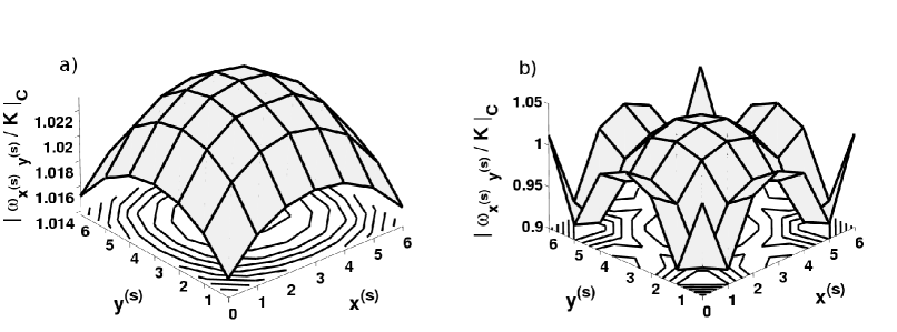
Figure 7: Critical ratio $\left|\omega_{x^{(s)}y^{(s)}}/K\right|_{C}$ for a two-dimensional lattice with $N=6$, $\epsilon_{s}$=0 and a) $\alpha=1.0$, b) $\alpha=100.0$.

The largest range for synchronized states is obtained if the pacemaker is either put in the center of the square (for open boundary conditions), or on a torus in two dimensions (as generalization of the closed ring in $d=1$ dimension). The different shape of the ”hats” at the boundaries is due to the dependence of the critical ratio on $\alpha$, in particular at the boundaries, as it was visible also in Fig.5. Recall that Eq. (9) was derived only for $\alpha\to\infty$.

IV Above the Critical Threshold

In this section we study the phase evolution of the oscillators when the ratio of the pacemaker’s eigenfrequency $\omega$ over the coupling $K$ lies above the threshold of phase-locked motion. As our numerical integration of the differential equations shows, there are still some regular remnants to phase-locked motion above the transition. Far above the transition the oscillators can no longer follow the pacemaker and get stuck to their eigenfrequency zero. These features are manifest in a phase portrait $\varphi_{i}(t)$ of all oscillators $i$ as a function of time, and in some average frequency $\overline{\Omega}(\omega)$ as a function of the pacemaker’s eigenfrequency $\omega$; $\overline{\Omega}$ replaces the common frequency $\Omega$ below the critical threshold. Its precise definition is given below. Here we consider only the one-dimensional ring-topology. We report our results in Figures 8 and 9.

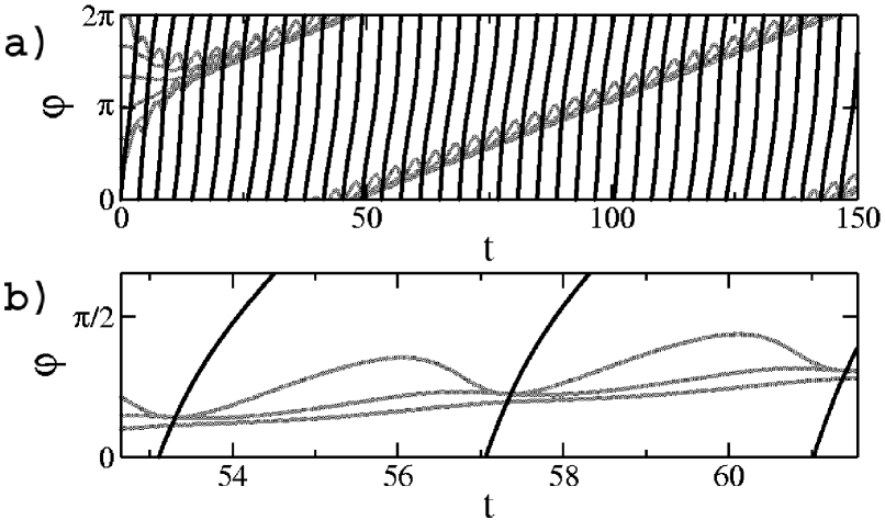
Figure 8: Phase portrait above the critical threshold ($\omega/K=2>\left|\omega/K\right|_{C}$) for $N=6$ oscillators on a ring with $\alpha=5.0$ and $\epsilon=0$. The almost vertical black lines represent the pacemaker’s phase, while the phases of the other oscillators are plotted with thin dark-grey lines. a) The pacemaker moves faster (steep slope) than the rest of the system that seems to move coherently with a common frequency; b) zooming into the phase portrait, it is clear that the phase of each of the oscillators different from the pacemaker oscillates around the common frequency with an amplitude inversely proportional to the distance from the pacemaker.

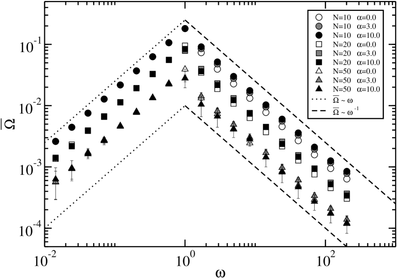
Figure 9: Dependence of the average frequency $\overline{\Omega}$ [Eq.(22)] as function of the pacemaker’s frequency $\omega$. Numerical results refer to the case of a ring, with $\epsilon=0$, $\omega>0$, $K=1$ and to different sizes of the system (i.e. different values of $N$) and/or ranges of the interactions (i.e. different values of $\alpha$). In this case, system (1) is integrated using the eight-order Runge-Kutta method with variable time step. Each point is given by the average over twenty different trials (for which the initial phases are chosen at random from a uniform distribution) and the error bars represent the standard deviation from the mean values. Error bars appear only from $N=50$ on and for $\alpha>0$, because the value of $t_{0}\sim 10^{3}$ is not always large enough to ensure that the system reaches the stable state for the given initial condition.

Phase portrait

Figure 8a shows the portrait of a non-synchronized ring with $N=6$, $\alpha=5.0$, $\epsilon=0$, and $\left|\omega/K\right|=2.0>\left|\omega/K\right|_{C}$. The phases $\varphi$ are projected to the interval $[0,2\pi)$. The fat vertical lines represent the phase evolution of the pacemaker, while the thin dark-grey lines correspond to the phase evolution of all other oscillators which seem to almost coincide along these lines, but a zoom, shown in Figure 8b, displays their difference in amplitudes as well as the superposition of a fast and a slow motion. Rewriting the differential equation for the $i$-th oscillator from system (1), with periodic boundary conditions, as

$$\dot{\varphi}_{i}=\frac{K}{\eta}\frac{\sin{\left(\varphi_{s}-\varphi_{i}\right)}}{r_{si}^{\alpha}}+\frac{K}{\eta}\sum_{j\neq s,i}\frac{\sin{\left(\varphi_{j}-\varphi_{i}\right)}}{r_{ji}^{\alpha}}\;\;\;,\;\forall\;i\neq s\;\;\;,$$ (20)

we can distinguish the interaction between the $i$-th oscillator and the pacemaker from the interactions between the $i$-th oscillator and the rest of the system. Calculating from Eq.(20) the average frequency $\overline{\Omega}$ of all the oscillators different from the pacemaker

$$\overline{\Omega}:=\frac{1}{N}\sum_{i\neq s}\dot{\varphi}_{i}=\frac{K}{N\eta}\sum_{i\neq s}\frac{\sin{\left(\varphi_{s}-\varphi_{i}\right)}}{r_{si}^{\alpha}}\;\;\;,$$ (21)

we see that $\overline{\Omega}$ is given by a weighted average of the interactions between the pacemaker and the other oscillators, without any contribution from the mutual interactions between oscillators different from the pacemaker.
Numerically we approximated the average frequency of Eq.(21) as

$$\overline{\Omega}=\frac{1}{N}\sum_{i\not=s}\frac{\varphi_{i}(t_{0}+t_{1})-\varphi_{i}(t_{0})}{t_{1}-t_{0}}\;\;\;,$$ (22)

with $10^{5}\sim t_{1}\gg t_{0}\sim 10^{3}$. The values of $t_{1}$ and $t_{0}$ are chosen sufficiently large to capture only the slow motion ($2\pi/(t_{1}-t_{0})\ll\omega$). Note that $\overline{\Omega}$ reduces to $\Omega$ when $\left|\omega/K\right|\leq\left|\omega/K\right|_{C}$, since in the phase-locked regime $\frac{\varphi_{i}(t_{0}+t_{1})-\varphi_{i}(t_{0})}{t_{1}-t_{0}}=\Omega\;\;\;,\;\forall\;i$.

Average frequency as a function of the pacemaker’s eigenfrequency

Moreover, it is of interest to study the absolute value of the average frequency $\overline{\Omega}$ as a function of the pacemaker’s eigenfrequency $\omega$, see Figure 9, where we have chosen $K=1$ for simplicity as well as $\omega>0$. For $\omega\leq\omega_{C}\simeq 1$ we obtain the linear increase of $\overline{\Omega}=\Omega\propto\omega$, as we expect from Eq.(4). For $\omega\to\infty$ we expect $\overline{\Omega}\to 0$, since the oscillators can no longer follow the pacemaker when its eigenfrequency goes to infinity. However, we have no analytical understanding of the decay of $\overline{\Omega}$ as an inverse power of $\omega$, $\overline{\Omega}\propto\omega^{-1}$ for $\omega\gg 1$. The dotted envelopes mark $\overline{\Omega}\propto\omega$, while the dashed curves correspond to $\overline{\Omega}\propto\omega^{-1}$. The numerical results show a weak dependence on the interaction range ($\alpha$ varies between $0$ and $10$), as well as a stronger dependence on the size $N$ of the system [for $\omega\leq\omega_{C}$ as predicted by Eq.(4)], $N$ varying between $10$ and $50$. For the numerical integration of the differential equations we used the eight-order Runge-Kutta algorithm with adapted time steps in order to accelerate the integration with variable time step. This introduces some “noise” in the numerical estimate of the first derivatives. Each data point corresponds to an unweighted average over twenty different choices of the initial phases (i.e. chosen at random from a uniform distribution). (To achieve a complete independence on the choice of initial conditions and a full stabilization would need a longer simulation time.) The size of the errors increases with $N$ as indicated in Figure 9.

V Summary and Conclusions

We considered ensembles of Kuramoto oscillators with zero eigenfrequency apart from one, the so-called pacemaker, with eigenfrequency larger than zero and coupled to the others in a symmetric ($\epsilon_{s}=0$) or asymmetric ($-1\leq\epsilon<0$) way. The oscillators were assigned to d-dimensional regular topologies, in particular to a one-dimensional open chain, a one-dimensional ring, a Cayley-tree with $z$ branches and a hypercubic lattice in $d$ dimensions. In general, we studied the conditions for having phase-locked motion as a function of the system size $N$, the coupling strength $K$, the pacemaker’s eigenfrequency $\omega_{s}$ and the asymmetry parameter $\epsilon_{s}$. The interaction range between the oscillators was varied between next-neighbor and all-to-all couplings via the parameter $\alpha$. We derived the common frequency $\Omega$ of the phase-locked motion, and the critical threshold $\left|\omega_{s}/K\right|_{C}$, analytically for the limiting cases $\alpha\to\infty$ and $\alpha=0$, in particular for a chain with arbitrary position of the pacemaker and a ring in one dimension, as well as for a Cayley-tree with coordination number $z\geq 2$. Intermediate coupling ranges $0<\alpha<\infty$ and the phase evolution above the critical threshold for phase-locked motion were treated numerically.
In the large $N$ limit, phase-locked motion is impossible in all cases we have considered, that is, for both chain- and ring- topologies, and for symmetric $(\epsilon_{s}=0)$ and asymmetric $(-1\leq\epsilon_{s}<0)$ couplings of the pacemaker. For $(\epsilon=-1)$, the common frequency $\Omega$ converges to the pacemaker’s $\omega_{s}$, but $\left|\omega_{s}/K\right|_{C}$ goes to zero for $N\to\infty$, whereas for $\epsilon=0$ $\Omega$ goes to zero while $\left|\omega_{s}/K\right|_{C}$ goes to one for $N\to\infty$. Similarly, on a Cayley-tree, which we studied for $\epsilon_{0}=0$, $\Omega$ and $\left|\omega_{0}/K\right|_{C}$ go to zero for $N\to\infty$, independently of whether the limit is realized as $z\to\infty$, or $R\to\infty$, or both. However, we were not only interested in the ”thermodynamic” limit and do not mean the transition to the desynchronized phase for finite $N$ in the thermodynamic sense of a phase transition. Our main result for finite $N$ and $-1\leq\epsilon\leq 0$ was that for a whole range of ratios $\left|\omega_{s}/K\right|$ it is possible to induce synchronization by a mere closure of a chain to a ring. (For ratios below this range the system synchronizes even for an open chain with pacemaker at position $s$, for ratios above this range synchronization is neither possible on a ring.)

Two interesting results were obtained from the numerical integration of the differential equations. Firstly, as a function of the interaction range (parameterized by $\alpha$), the critical ratio $\left|\omega/K\right|_{C}$ showed a minimum at some intermediate value around $\alpha_{M}\leq 3$ (for given $N$ and $\epsilon$ that we considered). This non-monotonic shape was obtained for our choice of normalization $\eta_{i}$, defined in Eq.(2). For the pacemaker it is therefore as easy to entrain the phases of the other oscillators if it only interacts with nearest neighbors as if it interacts with all other oscillators as nearest neighbors (mean-field case). This is well understandable from Eq.s(24) and (25) in the Appendix, from which it is seen that it is sufficient for the pacemaker to entrain its nearest neighbors in order to entrain all other oscillators. Formulas (24) and (25) were derived under the condition of nearest-neighbor interactions. Therefore the argument does not go through for intermediate values of $\alpha$, for which the numerical results show that the pacemaker has a ”harder job” to entrain the remaining ensemble.

Secondly, above the transition from the phase-locked motion to the desynchronized phase, we found some regular remnants of phase-locked motion. It is still the pacemaker that determines the fast frequency of phase fluctuations of the others around some average value $\overline{\Omega}$ (also determined by the pacemaker), and it is the distance to the pacemaker that determines the amplitude of these fluctuations. The value of the average frequency $\overline{\Omega}$ varies slowly as compared to the pacemaker’s frequency $\omega$. As expected, $\overline{\Omega}$ approaches zero for $\left|\omega/K\right|_{C}\to\infty$ as an expression of the fact that the system can no longer follow the pacemaker in this limit. The simple power-law of the decrease of $\overline{\Omega}$ remains to be understood analytically.
The sensitive dependence of synchronization on the topology in a certain range of parameters may be exploited in artificial networks and is -very likely- already utilized in natural systems, in which a switch to a synchronized state should be easily feasible.

Appendix

Kuramoto Model on a $d$-dimensional lattice

We start with the system given by Eq.s(1) and (2), defined on a $d$-dimensional lattice. Imposing the phase-locked condition

$$\dot{\varphi}_{i}\equiv\Omega\;\;\;,\;\forall\;i=0,\ldots,N\;\;\;\;\;\;,$$

we have

$$\Omega=\delta_{i,s}\omega_{s}+(1+\delta_{i,s}\epsilon_{s})\ \frac{K}{\eta_{i}}\ \Omega_{i}\;\;\;,\;\forall\ i=0,\ldots,N\;\;\;,$$

where

$$\Omega_{i}:=\sum_{j\not=i}\frac{\sin{(\varphi_{j}-\varphi_{i})}}{r_{ji}^{\alpha}}\;\;\;.$$

Common frequency in the phase-locked regime

As it is easily seen from the odd parity of the sine function,

$$\sum_{i}\Omega_{i}=0\ \ \textrm{ and }\ \ \sum_{i\neq g}\Omega_{i}=-\Omega_{g}\;,$$

so that

$$\begin{array}[]{l}\sum_{i\neq s}\Omega\frac{\eta_{i}}{K}=\sum_{i\neq s}\delta_{i,s}\frac{\eta_{i}\omega_{s}}{K}+\sum_{i\neq s}(1+\delta_{i,s}\epsilon_{s})\Omega_{i}\\ \Rightarrow\ \frac{\Omega}{K}\sum_{i\neq s}\eta_{i}=-\Omega_{s}\end{array}\;\;\;,$$

while for $j\neq s$

$$\begin{array}[]{l}\sum_{i\neq j}\Omega\frac{\eta_{i}}{K}=\sum_{i\neq j}\delta_{i,s}\frac{\eta_{i}\omega_{s}}{K}+\sum_{i\neq j}(1+\delta_{i,s}\epsilon_{s})\Omega_{i}\\ \Rightarrow\ \frac{\Omega}{K}\sum_{i\neq j}\eta_{i}=\frac{\eta_{s}\omega_{s}}{K}-\Omega_{j}+\epsilon_{s}\Omega_{s}\\ \Rightarrow\ \frac{\Omega}{K}\sum_{j\neq s}\sum_{i\neq j}\eta_{i}=\sum_{j\neq s}\frac{\eta_{s}\omega_{s}}{K}-\sum_{j\neq s}\Omega_{j}+\sum_{j\neq s}\epsilon_{s}\Omega_{s}\\ \Rightarrow\ \frac{\Omega}{K}\sum_{j\neq s}\sum_{i\neq j}\eta_{i}=\frac{N\eta_{s}\omega_{s}}{K}+(1+\epsilon_{s}N)\Omega_{s}\end{array}\;\;\;,$$

which implies

$$\frac{\Omega}{K}\Big{[}(1+\epsilon_{s}N)\sum_{i\neq s}\eta_{i}+\sum_{j\neq s}\sum_{i\neq j}\eta_{i}\Big{]}=\frac{N\eta_{s}\omega_{s}}{K}\;\;\;.$$

The common frequency $\Omega$ then follows as in Eq.(3).
When the topology has a symmetry such that the normalization factor defined in Eq.(2) is independent of the index $i$

$$\eta_{i}\equiv\eta\;\;\;,\;\forall\;i=0,\ldots,N\;\;\;,$$

then

$$\left(1+\epsilon N\right)\sum_{i\neq s}\eta+\sum_{j\neq s}\sum_{i\neq j}\eta=\left(1+\epsilon N\right)N\eta+N^{2}\eta=N\eta\left(N+\epsilon N+1\right)\;\;\;,$$

thus we obtain Eq.(4).
Such symmetries are realized for $\alpha=0$, and for arbitrary $\alpha$ if we have periodic boundary conditions.

Critical ratio $\left|\omega_{s}/K\right|_{C}$ for the one-dimensional lattice

In the case of next-neighbor interactions (i.e. for $\alpha\rightarrow\infty$), on an open chain, we can solve the system (1) recursively. We start from the equation for the pacemaker (assuming $0<s<N$ and $\epsilon_{s}\neq-1$) and move first to the right of the pacemaker

$$\begin{array}[]{l}\Omega=\frac{K}{2}\Big{[}\sin{(\varphi_{s}-\varphi_{s+1})}+\sin{(\varphi_{s+2}-\varphi_{s+1})}\Big{]}\\ \Leftrightarrow\ \sin{(\varphi_{s+2}-\varphi_{s+1})}=\frac{2\Omega}{K}+\sin{(\varphi_{s+1}-\varphi_{s})}\;.\end{array}$$

For all $\ 1\leq j\leq N-s$ it then follows that

$$\begin{array}[]{l}\Omega=\frac{K}{2}\Big{[}\sin{(\varphi_{s+(j-2)}-\varphi_{s+(j-1)})}+\\ \quad+\sin{(\varphi_{s+j}-\varphi_{s+(j-1)})}\Big{]}\\ \Leftrightarrow\ \sin{(\varphi_{s+j}-\varphi_{s+(j-1)})}=\\ =\frac{2\Omega}{K}+\sin{(\varphi_{s+(j-1)}-\varphi_{s+(j-2)})}=\\ =(j-1)\frac{2\Omega}{K}+\sin{(\varphi_{s+1}-\varphi_{s})}\end{array}\;\;\;\;.$$

In particular for $j=N-s$, we have

$$\sin{(\varphi_{N}-\varphi_{N-1})}=(N-s-1)\frac{2\Omega}{K}\sin{(\varphi_{s+1}-\varphi_{s})}\;.$$

Imposing the boundary conditions

$$\begin{array}[]{l}\Omega=K\sin{(\varphi_{N-1}-\varphi_{N})}\\ \Leftrightarrow\ \sin{(\varphi_{N-1}-\varphi_{N})}=\frac{\Omega}{K}\;\;,\end{array}$$

we obtain for all $1\leq j\leq N-s$

$$\sin{(\varphi_{s+j}-\varphi_{s+(j-1)})}=(2s-2N-1)\frac{\Omega}{K}+2j\frac{\Omega}{K}\;\;\;,$$ (23)

which implies Eq.(6) by imposing the condition that the sine is a bounded function ($|\sin x|\leq 1$). When $\omega_{s}>0$ [$\omega_{s}<0$], Eq.(23) is always negative [positive] and has its minimum [maximum] value for $j=1$. So if

$$\begin{array}[]{ll}\sin{(\varphi_{s+1}-\varphi_{s})}\geq-1&\textrm{ , if }\omega_{s}>0\\ \sin{(\varphi_{s+1}-\varphi_{s})}\leq 1&\textrm{ , if }\omega_{s}<0\end{array}\Longleftrightarrow\left|\sin{(\varphi_{s+1}-\varphi_{s})}\right|\leq 1\;\;\;,\;\forall\;\omega_{s}\neq 0$$ (24)

then

$$\begin{array}[]{ll}\sin{(\varphi_{s+j}-\varphi_{s+(j-1)})}\geq-1&\textrm{ , if }\omega_{s}>0\\ \sin{(\varphi_{s+j}-\varphi_{s+(j-1)})}\leq 1&\textrm{ , if }\omega_{s}<0\end{array}\Longleftrightarrow\left|\sin{(\varphi_{s+j}-\varphi_{s+(j-1)})}\right|\leq 1\;\;\;,\;\forall\;\omega_{s}\neq 0\;\;\;,$$ (25)

$\forall\;1\leq j\leq N-s$. In other words, if the first neighbor on the right hand side of the pacemaker (the $(s+1)$-th oscillator) follows the pacemaker [i.e. if Eq.(24) is satisfied], then all the others follow the pacemaker with the same velocity [i.e. Eq.(25) is also satisfied].
In the same way we obtain Eq.(7) for oscillators to the left of the pacemaker. Of course we need that both the left and the right parts are synchronized in frequency, hence Eq.(8) is the global solution.
Eq.(9), for which the pacemaker is at the first ($s=0$) [or at the last ($s=N$)] position of the chain, is obtained in the same way, but in these particular cases only a motion to the right [or to the left] is possible because the left [or the right] part does not exist. In case of the ring the procedure for deriving Eq.(14) is the same, apart from applying the different boundary conditions, periodic ones in this case.

For $\alpha=0$ and phase-locked conditions, the system (1) and (2) becomes

$$\Omega=\delta_{i,s}\omega_{s}+(1+\delta_{i,s}\epsilon_{s})\frac{K}{N}\sum_{j}\sin{(\varphi_{j}-\varphi_{i})}\;\;\;.$$

Introducing the definition of Eq.(15) (which serves as an order parameter in a mean-field approximation that here becomes exact), we write

$$\left\{\begin{array}[]{l}\Omega=\omega_{s}+(1+\epsilon_{s})KR\sin{(\psi-\varphi_{s})}\;\;\;for\;\;i=s\\ \Omega=\frac{K}{N}\sin{(\varphi_{s}-\varphi_{i})}+KR\sin{(\psi-\varphi_{i})}\;\;\;,\;\forall\;i\neq s\end{array}\right.\;\;\;\;.$$

Here all oscillators different from the pacemaker satisfy exactly the same equation. One possible solution is that all the phases of the oscillators different from the pacemaker are equal

$$\varphi_{i}\equiv\psi\;\;\;,\;\forall\;i\neq s\;\;\;,$$

from which it follows that

$$\Omega=\frac{K}{N}\sin{(\varphi_{s}-\varphi_{i})}\;\;\;,\;\forall\;i\neq s\;\;.$$

Using the last equation, the fact that the sine-function is bounded and finally the value of the common frequency, previously calculated in Eq.(4), it is straightforward to derive Eq.(14).

Kuramoto Model on a Cayley Tree

Consider a node at distance $R$ from the pacemaker, reached along the path $(s_{1},s_{2},s_{3},\ldots,s_{R-1},s_{R})$ from the central node. Here $s_{1}=1,\ldots,z$ , while $s_{i}=1,\ldots,z-1$ , $\forall i=2,\dots,R$. For this node we can write Eq. (17) as

$$\begin{array}[]{l}\dot{\varphi}_{R,s_{1},s_{2},\ldots,s_{R-1},s_{R}}=\Omega=\\ =K\sin{(\varphi_{R-1,s_{1},s_{2},\ldots,s_{R-1}}-\varphi_{R,s_{1},s_{2},\ldots,s_{R-1},s_{R}})}\\ \Leftrightarrow\ \sin{(\varphi_{R-1,s_{1},s_{2},\ldots,s_{R-1}}-\varphi_{R,s_{1},s_{2},\ldots,s_{R-1},s_{R}})}=\frac{\Omega}{K}\end{array}\;\;\;\;,$$

from which we can see that all oscillators at distance $R$, independently on the path along which they are reached from the center, satisfy the same equation.
Proceeding in an analogous way to before, we can write

$$\begin{array}[]{l}\dot{\varphi}_{R-1,s_{1},s_{2},\ldots,s_{R-2},s_{R-1}}=\Omega=\\ =\frac{K}{z}\Big{[}\sum_{s_{R}=1}^{z-1}\ \sin{(\varphi_{R,s_{1},s_{2},\ldots,s_{R-1},s_{R}}-\varphi_{R-1,s_{1},s_{2},\ldots,s_{R-1}})}+\\ \quad+\sin{(\varphi_{R-2,s_{1},s_{2},\ldots,s_{R-2}}-\varphi_{R-1,s_{1},s_{2},\ldots,s_{R-1}})}\Big{]}=\\ =\frac{K}{z}\Big{[}-(z-1)\frac{\Omega}{K}+\sin{(\varphi_{R-2,s_{1},s_{2},\ldots,s_{R-2}}-\varphi_{R-1,s_{1},s_{2},\ldots,s_{R-1}})}\Big{]}\\ \Leftrightarrow\ \sin{(\varphi_{R-2,s_{1},s_{2},\ldots,s_{R-2}}-\varphi_{R-1,s_{1},s_{2},\ldots,s_{R-1}})}=\frac{\Omega}{K}[z+(z-1)]\;\;,\end{array}$$

next

$$\begin{array}[]{l}\dot{\varphi}_{R-2,s_{1},s_{2},\ldots,s_{R-2}}=\Omega=\\ \frac{K}{z}\Big{[}\sum_{s_{R-1}=1}^{z-1}\ \sin{(\varphi_{R-1,s_{1},s_{2},\ldots,s_{R-2},s_{R-1}}-\varphi_{R-2,s_{1},s_{2},\ldots,s_{R-2}})}+\\ +\sin{(\varphi_{R-3,s_{1},s_{2},\ldots,s_{R-3}}-\varphi_{R-2,s_{1},s_{2},\ldots,s_{R-2}})}\Big{]}=\\ =\frac{K}{z}\Big{[}-(z-1)\frac{\Omega}{K}[z+(z-1)]+\sin{(\varphi_{R-3,s_{1},s_{2},\ldots,s_{R-3}}-\varphi_{R-2,s_{1},s_{2},\ldots,s_{R-3},s_{R-2}})}\Big{]}\\ \Longrightarrow\ \sin{(\varphi_{R-3,s_{1},s_{2},\ldots,s_{R-3}}-\varphi_{R-2,s_{1},s_{2},\ldots,s_{R-3},s_{R-2}})}=\frac{\Omega}{K}[z+z(z-1)+(z-1)^{2}]\end{array}$$

and so on, until we arrive at

$$\sin{(\varphi_{R-(t+1),s_{1},s_{2},\ldots,s_{R-(t+1)}}-\varphi_{R-t,s_{1},s_{2},\ldots,s_{R-(t+1)},s_{R-t}})}=\frac{\Omega}{K}\ [\ z\ \sum_{q=0}^{t-1}\ (z-1)^{q}\ +\ (z-1)^{t}\ ]\;\;\;\;.$$

For $t=R-1$, we have

$$\sin{(\varphi_{0}-\varphi_{1,s_{1}})}=\frac{\Omega}{K}\ [\ z\ \sum_{q=0}^{R-2}\ (z-1)^{q}\ +\ (z-1)^{R-1}\ ]\;\;\;\;,$$

but also, at the center of the Cayley tree,

$$\Omega=\dot{\varphi}_{0}=\omega_{0}+\frac{K}{z}\ \sum_{s_{1}=1}^{z}\ \sin{(\varphi_{1,s_{1}}-\varphi_{0})}=\omega_{0}-K\ \frac{\Omega}{K}\ [\ z\ \sum_{q=0}^{R-2}\ (z-1)^{q}\ +\ (z-1)^{R-1}\ ]\;\;\;.$$ (26)

Eq.(18) is easily obtained from Eq.(26).
As we have seen, all oscillators at the same distance $r$ from the pacemaker satisfy the same equation. We can write

$$\sin{(\varphi_{r}-\varphi_{r-1})}\ =\ -\ \frac{\omega_{0}}{K}\ \frac{z\ \sum_{q=0}^{R-r-1}\ (z-1)^{q}\ +\ (z-1)^{R-r}}{\ 1\ +\ z\ \sum_{q=0}^{R-2}\ (z-1)^{q}\ +\ (z-1)^{R-1}}\;\;\;\;,$$

suppressing the path that was followed to reach the node. It is convenient to rewrite this equation according to

$$\begin{array}[]{l}z\ \sum_{q=0}^{R-r-1}\ (z-1)^{q}\ +\ (z-1)^{R-r}=\\ =\frac{1}{(z-1)^{r-1}}\Big{[}z\sum_{q=0}^{R-r-1}(z-1)^{q+r-1}+(z-1)^{R-r+r-1}\Big{]}=\\ =\ \frac{1}{(z-1)^{r-1}}\Big{[}z\sum_{s=r-1}^{R-2}\ (z-1)^{s}\ +\ (z-1)^{R-1}\Big{]}\ =\\ =\ \frac{1}{(z-1)^{r-1}}\Big{[}z\sum_{s=0}^{R-2}\ (z-1)^{s}\ -\ z\sum_{s=0}^{r-2}\ (z-1)^{s}\ +\ (z-1)^{R-1}\Big{]}\ =\\ =\ \frac{1}{(z-1)^{r-1}}\Big{[}1\ +\ z\sum_{s=0}^{R-2}\ (z-1)^{s}\ +\ (z-1)^{R-1}\ -\ z\sum_{s=0}^{r-2}\ (z-1)^{s}\ -\ 1\Big{]}\end{array}\ \ .$$

for $R\geq 2$. Finally we obtain

$$\sin{(\varphi_{r}-\varphi_{r-1})}\ =\frac{\omega_{0}}{K\ (z-1)^{r-1}}\ \Big{[}\ \frac{1\ +\ z\ \sum_{s=0}^{r-2}\ (z-1)^{s}}{1\ +\ z\ \sum_{s=0}^{R-2}\ (z-1)^{s}\ +\ (z-1)^{R-1}}\ -\ 1\ \Big{]}\;\;.$$ (27)

When $\omega_{0}>0$, Eq. (27) is always negative, monotone and increasing and takes its minimum value for $r=1$, while when $\omega_{0}<0$, Eq. (27) is always positive, monotone and decreasing and takes its maximum value for $r=1$, namely

$$\sin{(\varphi_{1}-\varphi_{0})}\ =\ \frac{\omega_{0}}{K}\ \Big{[}\ \frac{1}{1\ +\ z\ \sum_{s=0}^{R-2}\ (z-1)^{s}\ +\ (z-1)^{R-1}}\ -\ 1\ \Big{]}\;\;\;\;.$$

In order to derive the maximal value for $\left|\omega_{0}/K\right|$, we use the bound on sine function, from which we find the critical fraction of Eq.(19).

References

• (1) J. Buck, Nature 211, 562 (1966).
• (2) T.J. Walker, Science 166, 891 (1969).
• (3) Y. Kuramoto ”Chemical Oscillators, Waves, and Turbolence”, (Springer New York 1984).
• (4) A.T. Winfree , ”The geometry of biological time” , (Springer-Verlag New York 1980).
• (5) J.A. AcebrΓ³n, L.L. Bonilla, C.J. PΓ©rez-Vicente, F. Ritort, and R. Spigler, Rev. Mod. Phys. 77, 137 (2005).
• (6) H. Yamada, Prog. Theor. Phys. , 108 (2002).
• (7) H. Daido , Phys. Rev. Lett. 61 , 231 , (1988).
• (8) S.H. Strogatz , and R.E. Mirollo , J. Phys. A: Math. Gen. 21 , L699 , (1988).
• (9) J. Rogers , L.T. Wille , Phys. Rev. E 54 , R2192-R2196, (1996).
• (10) A. Bunde , and S. Havlin , ”Fractals and disordered systems” , (Springer-Verlag Berlin 1991).
• (11) S.H. Yook , and H. Meyer-Ortmanns , preprint cond-mat/0507422 , (2005).