Slip, immiscibility and boundary conditions at the liquid-liquid interface

Abstract

The conventional boundary conditions at the interface between two flowing liquids include continuity of the tangential velocity. We have tested this assumption with molecular dynamics simulations of Couette and Poiseuille flows of two-layered liquid systems, with various molecular structures and interactions. When the total liquid density near the interface drops significantly compared to the bulk values, the tangential velocity varies very rapidly there, and would appear discontinuous at continuum resolution. The value of this apparent slip is given by a Navier boundary condition.

Recent studies of the nanoscale behavior of flowing fluids have reinvigorated interest in the nature and validity of the boundary conditions which accompany the Navier-Stokes equations. The velocity condition at a solid-liquid interface, and the possibility of slip there, has been a particular focus lauga due to its relevance in possible “lab on a chip” and other devicesgc ; ssa . At a liquid-liquid interface the conventional boundary condition is also no-slip. An obvious physical argument is that the interface between the two liquids is actually a region whose thickness is at least a few molecular diameters, where molecules of both materials are present and interacting with each other. It is difficult to imagine how two intermixed dense liquids could maintain distinct molecular speeds, and one expects a single velocity for both liquids in the interface, and that this velocity would vary smoothly in moving from the interface into either bulk region as the species concentrations change gradually. In the light of the examples of solid-liquid slip cited above, this argument might fail when interfacial mixing is poor and the molecules of different species are spatially separated. For simple liquids, we are not aware of any experimental measurements or systematic computational studies of liquid-liquid slip at all, although for polymer melts there is by now convincing indirect zm and direct lam evidence for slip. The former study is based on the interpretation of measurements of pressure drop vs. shear rate in extrusion, and the latter on confocal microscopic observation with a spatial resolution of about 10$\mu$m. At the molecular scale, there are MD simulations for model polymers br and self-consistent field theory calculations lo which find slip, but no direct experimental results.

To investigate the question of liquid-liquid slip on a fundamental microscopic basis, we have conducted molecular dynamics (MD) simulations of the Couette and Poiseuille flows of two-layered immiscible liquid systems for a number of simple choices of interactions and molecular architecture. Standard MD techniques at ; kb95 are used, and the computational details are similar to those of Refs. ckb . The basic interatomic potential of Lennard-Jones form, $V_{ij}(r)=4\epsilon\left[(r/\sigma)^{-12}-A_{ij}(r/\sigma)^{-6}\right]$, where $r$ is the interatomic separation, $\sigma$ is roughly the size of the repulsive core, of order a few Angstroms, $\epsilon$ is the strength of the potential and $A_{ij}=A_{ji}$ is a dimensionless parameter that controls the attraction between atoms of atomic species $i$ and $j$. Numerical results are expressed in terms of the length scale $\sigma$ (a few Angstroms), the atomic mass $m$, and a time scale $\tau=\sigma(m/\epsilon)^{1/2}$, a few picoseconds. Temperature is controlled by a Nosé-Hoover thermostat, and the atoms are in many cases grouped into flexible chain molecules using a FENE potential $V_{\rm FENE}(r)=-(k/2)\ln\left[1-{r^{2}/r_{0}^{2}}\right]$ with maximum bond length $r_{0}=1.5\sigma$ and spring constant $k=30\epsilon/\sigma^{2}$. The liquids are confined between solid walls, each made of a layer of fcc unit cells whose atoms are tethered to lattice sites with a stiff linear spring. Periodic boundary conditions are applied in the two lateral directions. Couette flow is achieved by translating the upper and lower wall tether sites at constant velocity $\pm U$, and Poiseuille flow results from applying an acceleration $g$ parallel to the walls to each liquid atom.

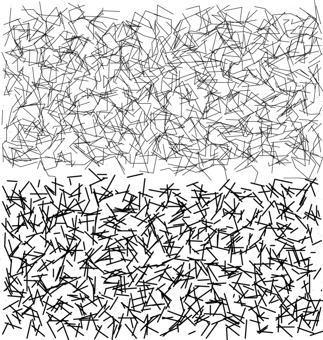
Figure 1: Interfacial region for the (2,4) system for miscible (top) and immiscible (bottom) interactions. The figure shows a three dimensional slab centered on the interface, as viewed from a long distance. Molecules are represented by the line segments joining the atomic centers, using thick/thin lines for dimer/tetramer molecules. The width of the system is 17.1$\sigma$, and the instantaneous gap between the upper and lower liquids in the immisicble case is 0.5-1.0$\sigma$.

The different simulated systems are characterized by the interaction coefficients $A_{ij}$ and the lengths $\ell_{1}$ and $\ell_{2}$ – the number of atoms per chain – of the two species of liquid molecule. The interactions are either immiscible, with $A_{12}=0$ and all other $A_{ij}=1$, or partially miscible as given by the Lorentz-Berthelot combination rules at , with $A_{11}=5/4$, $A_{22}=3/4$, and $A_{12}=\sqrt{A_{11}\,A_{22}}=0.97$. Although the interactions are somewhat simplified as compared with realistic molecules, these systems exhibit a sufficient variety of behaviors to identify some trends. We have examined systems with both types of interactions, for the cases $(l_{1},l_{2})=(1,1)$, (2,4) and (4,16). In the first two cases, the simulated system consists of 4000 atoms of each fluid, and 576 solid atoms in each wall, and has length $17.1\sigma$ in the flow and neutral directions and $34.2\sigma$ between walls; the third system was twice as large in each dimension and has eight times the number of atoms. The simulated Reynolds numbers are $O(10^{-2}-1)$, and the Deborah number based on the characteristic atomic time $\tau$ is ${\rm De}=\dot{\gamma}\tau=O(10^{-2})$. We will discuss the results for the prototypical (2,4) case in some detail. Numerical results are summarized in Table I below.

A crucial feature of these two-liquid systems is the microscopic structure of the interface, and in Fig. 1 we show a snapshot of the atoms in this region for the miscible and immiscible cases. In the miscible case atoms of the two molecules attract each other, so an overlap region separates the bulk liquids, whereas in the immiscible case the two types of atom repel each other, and there is an open gap. The time-averaged density profiles in Fig. 2 reflect this behavior: in the miscible case the density varies monotonically from one bulk value to the other whereas the immiscible case shows a substantial dip in density in the interfacial region. A quantitative measure of this density dip used below is the the difference between the mean of the two bulk densities and the density at the interface, relative to the mean, $\delta=0.66$ in this case. In Couette flow, we see that the velocity profile for the miscible system consists of two straight segments with different slopes (reflecting the different viscosities of the two liquids) with a rounded transition located at the position of the interface. The shear stress (not shown) has a constant value throughout both liquids. In Poiseuille flow for the miscible system, the density profile is essentially unchanged, while the velocity profile Fig. 3 corresponds to two distinct parabolas with a smooth transition, and the shear stress has two straight segments of different slope (reflecting the different liquid densities) which join smoothly to produce a continuous function of position.

Figure 2: Density and velocity profiles in Couette flow for (2,4) systems. The coordinate $y$ runs normal to the interface, and the profiles average over the other two directions. In the density profiles, miscible (left) and immiscible (right), the ($\times$) symbols refer to the dimers and ($*$) to the tetramers, while the continuous curve is the total liquid density. In the velocity and other plots below, points labeled (o) and (+) refer to the miscible and immiscible systems, respectively.

In the immiscible case, while the velocity profiles are again continuous functions, they exhibit a very rapid transition in traversing the interface in both flows, while the shear stress has the same qualitative features as in the previous case. Note that in obtaining these density, velocity and stress profiles, we divide the region between the walls into very narrow slabs of thickness $0.17\sigma$ parallel to the interface and average over a 5000$\tau$ time interval. Most conceivable experiments and all continuum modeling will not have the sub-Angstrom spatial resolution of these simulations, and the smoothed step in the velocity field in the immiscible case would appear to be a discontinuity, which we would describe precisely as “apparent velocity slip.”

Figure 3: Velocity and shear stress profiles in Poiseuille flow for the (2,4) systems, with points marked by (o) and (+) miscible and immiscible respectively. In the stress plot, the straight lines are a linear fit to each liquid region.

System	Flow	$\Delta u$	$S$	$\alpha$	$\delta$
(1,1)	0.001 C	0.0029	0.0011	2.6	0.49
	0.05 C	0.014	0.0059	2.4	0.49
	0.1 C	0.031	0.012	2.6	0.49
	0.2 C	0.050	0.020	2.5	0.49
	0.01 P	0.0	0.0	–	0.49
(2,4)	0.05 C	0.038	0.0063	6.0	0.66
	0.1 C	0.070	0.012	5.8	0.66
	0.2 C	0.13	0.021	6.2	0.66
	0.01 P	0.071	0.012	5.9	0.66
	0.02 P	0.15	0.025	6.0	0.66
(4,16)	0.1 C	0.032	0.0099	3.2	0.46
	0.2 C	0.070	0.021	3.3	0.46
	0.01 P	0.15	0.049	3.0	0.46
	0.02 P	0.22	0.70	3.1	0.46

Table 1: Numerical results for slip. The notation is that $(l_{1},l_{2})$ refers to a liquid made of flexible chains of length $l_{1}$ in contact with a second liquid of chains of length $l_{2}$, with interactions either of the immiscible or miscible (LB) type. “0.1 C” means Couette flow with wall velocities $\pm$0.1, and ”0.01 P” means gravity driven Poiseuille flow with acceleration 0.01. $\Delta u$, $S$, $\alpha$ and $\delta$ are the apaprent slip, shear stress at the interface, Navier coefficient and relative density dip, respectively. All entries are in MD units.

It remains to characterize the velocity discontinuity in terms of a boundary condition suitable for continuum calculations. Following the history of the no-slip condition lauga , simple plausibility, and the results of Zhao and Macosko zm for polymer systems, we consider the Navier condition $\Delta u=\alpha\,S$, where $S$ is the shear stress at the position of the interface, and $\alpha$ is a slip coefficient that depends on the nature of the two liquids present. ($\alpha$ is the inverse of the coefficient $\beta$ introduced in zm .) In the (1,1) immiscible system, the two liquids are identical except for their mutual repulsion and have equal viscosities and densities, so that the interface lies exactly in the middle of the channel. In Poiseuille flow, the shear stress then vanishes at the interface, and the Navier condition predicts no velocity discontinuity, exactly as seen in the simulations.

In Table I, we evaluate the slip coefficient from the MD data in the various cases simulated. The key feature of the Table is the approximately constant value of $\alpha$ obtained for each liquid pair, independent of the flow configuration and the value of the driving force. The numerical values have not been determined with very high precision, partly due to statistical fluctuations in the shear stress, and partly due to uncertainties in extrapolating across the interfacial region, but the trend is clear. At sufficiently high shear rates, non-Newtonian effects would appear, and $\alpha$ might vary accordingly, as found in zm . We conclude that the Navier condition is an appropriate and genuine boundary condition for a liquid-liquid interface.

An outstanding issue is the value of the slip coefficient $\alpha$. If we use parameter values for Argon (for which the Lennard-Jones potential with $A_{ij}=1$ is quantitatively valid) to translate the (1,1) coefficient into physical units, we have $\alpha\sim 10^{-5}$m/Pa s, a value three orders of magnitude larger than observed or inferred in polymer melts lam ; zm at low shear rates. A likely explanation for the discrepancy is that the interactions used here may be too repulsive as compared to those in the experimental systems. To pursue this possibility, in the (2,4) system we ran additional simulations with decreasing immiscibility, using a sequence of higher values of the inter-liquid interaction strengh $A_{12}=0.2\ldots 0.8$. The apparent slip and the density dip were found to decrease roughly linearly to zero from their values at $A_{12}=0$ in Table I. More generally, $\alpha$ depends in a non-trivial way on the molecular structure and interaction of both fluids present at the interface, as well as operating conditions such as temperature and density, and perhaps on driving force as well at higher shear and velocity, and little insight into its value is available at the moment.

A dip in the density at a liquid-liquid interface is somewhat unusual, and in the light of the preceding paragraph one may be concerned about the realism of the Lennard-Jones potentials used in this paper. In fact, simulations in the literature using fairly realistic interactions either do or do not exhibit a dip, depending on the liquids involved: for example, a dip is present at the water/octane interface octane but not in the water/carbon tetrachloride case ccl4 . Experimental evidence for a density dip is lacking, but an experimental measurement is difficult. While it is possible to obtain high resolution normal to an interface using x-ray scattering for example, the horizontal resolution is much coarser, and at larger length scales an interface is subject to thermal roughening which would smooth the density profile.

We thank M. M. Denn and M. Rauscher for discussions. This work was supported by the NASA Exploration Systems Mission Directorate.

References

- (1) A recent survey is E. Lauga, M. P. Brenner and H. A. Stone, cond-mat/0501557, to appear in Handbook of Experimental Fluid Dynamics, ed. J. Foss, C. Tropea and A. Yarin (Springer, New York, 2005).
- (2) N. Giordano and J.-T. Cheng, J. Phys.:Condens. Matter 13, R271 (2001).
- (3) H. A. Stone, A. D. Stroock and A. Adjari, Annu. Rev. Fluid Mech. 36, 381 (2004).
- (4) R. Zhao and C. W. Macosko, J. Rheol. 46, 145 (2002).
- (5) Y. C. Lam, et al., J. Rheol. 47, 795 (2003).
- (6) S. Barsky and M. O. Robbins, Phys. Rev. E 63, 021801 (2001); ibid. 65, 021808 (2002).
- (7) T. S. Lo, M. Mihajlovic, Y. Schnidman, W. Li and D. Gersappe, Phys. Rev. E 72, 040801 (2005).
- (8) M. P. Allen and D. J. Tildesley, Computer Simulation of Liquids (Clarendon, Oxford, 1987).
- (9) J. Koplik and J. R. Banavar, Annu. Rev. Fluid Mech. 27, 257 (1995).
- (10) M. Cieplak, J. Koplik and J. R. Banavar, Phys. Rev. Lett. 86, 803 (2001).
- (11) H. A. Patel, E. B. Nauman and S. Garde, J. Chem. Phys. 119, 9199 (2003).
- (12) S. Senapati and M. L. Berkowitz, Phys. Rev. Lett. 87, 176101 (2001).