Exploring the energy landscape of model proteins: a metric criterion for the determination of dynamical connectivity

Abstract

A method to reconstruct the energy landscape of small peptides is presented with reference to a 2d off–lattice model. The starting point is a statistical analysis of the configurational distances between generic minima and directly connected pairs (DCP). As the mutual distance of DCP is typically much smaller than that of generic pairs, a metric criterion can be established to identify the great majority of DCP. Advantages and limits of this approach are thoroughly analyzed for three different heteropolymeric chains. A funnel–like structure of the energy landscape is found in all of the three cases, but the escape rates clearly reveal that the native configuration is more easily accessible (and is significantly more stable) for the sequence that is expected to behave as a real protein.

I Introduction

Several states of matter are characterized by a rich energy landscape (EL), which, in turn, hints at peculiar structural and dynamical features. Supercooled liquids, glasses, atomic clusters and biomolecules wales are typical examples of systems whose complex thermodynamic behavior can be traced back to the intricate topological properties of the EL. The pioneering work by Stillinger and Weber on “inherent” structures of liquids still2 revealed the importance of investigating the stationary points of the EL for characterizing their dynamical and thermodynamic properties. Similar approaches have been proposed and successfully applied to the identification of the structural–arrest temperature in glasses sastry and supercooled liquids angelani .

More recently, this kind of analysis has been extended to the study of protein models krivov ; evans ; baumketner . They suggest that also the folding process of a protein towards its native configuration (NC) depends on the structure of its EL. This has been found to possess a funnel–like shape: the NC is located inside the so–called native valley (NV) at the bottom of the funnel funnel .

Below the folding temperature, the evolution from a coil state to the NC is determined by the propensity of the protein to enter the relatively small fraction of states composing the NV without having to visit the entire phase-space. In a statistical sense, the folding process can be viewed as a weighted sampling mechanism which favours specific intermediate configurations. They correspond to assembling the building blocks which eventually constitute the NC. Well above the folding temperature, no marked difference exists among the various states and the protein spends most of the time jumping between different random coil configurations.

In the absence of external forces, only thermal fluctuations can drive the protein dynamics through different regions of the EL. In particular, below the folding temperature, the protein is expected to evolve mainly inside the NV. Nonetheless, large deviations from the NC cannot be avoided, but they are both rare and very short lived. This scenario was confirmed by simulations performed in a 2d off–lattice modeltlp . A more detailed analysis of the model tap revealed that the protein dynamics can viewed as a sequence of jumps between pairs of minima separated by one saddle, that we call directly connected pairs (DCP). Each jump is a thermally activated process: the protein performs random oscillations in the basin of a local minimum until a sufficiently large thermal fluctuation allows it to overtake the energy barrier separating the minimum from a neighbouring one. In a high–dimensional space, the transition rate can be computed as the product of the Arrhenius factor times an entropic weight which depends on the DCP and on the saddle curvatures (see Section IV). In other words, the relevant information about the protein dynamics can be obtained from the knowledge of the DCP and of the corresponding saddles. However, the reconstruction of the EL is a very difficult task to be accomplished in practice. Indeed, the identification of DCP by a systematic exploration of the entire set of the $N$ identified minima requires to exploring $N^{2}$ pairs, which is already on the order of $10^{9}$ for the partial database generated (see the Appendix for a description of the algorithm) in the relatively small polypeptidic chains investigated in this paper (see section II). It is therefore, crucial to develop effective strategies for identifying DCP within the set of all, a priori possible, candidates. This is the main issue addressed in this paper.

It is reasonable to conjecture that the distance separating DCP is typically smaller than that between generic pairs of minima. It is therefore tempting to restrict the analysis to those pairs whose mutual distance is smaller than some prescribed threshold. However, whether this approach effectively works may depend on several factors one of which is the adopted definition of distance. For this reason, in section III we introduce and compare different conformational distances. It turns out that the bond–angle distance, defined by the absolute–value norm is the one that makes the implementation of such a criterion most accurate in the identification of DCP. The price one has to pay is that, unavoidably, all DCP characterized by a distance larger than the given threshold are missed. The detailed analysis of the EL dscribed in Section IV indicates that the average distance between DCP is larger for minima that are closer to the NC. Accordingly, the computational advantage guaranteed by the choice of a relatively small threshold could be frustrated by the loss of important connections located in the NV. For this reason, we argue that the distance criterion has to be complemented by a systematic search of all DCP involving minima in the NV, a much more accessible task, given the limited number of such minima (for an operative definition of the NV see section IV).

II The model

The model studied in this paper is a modified version of the 2d off-lattice model introduced by Stillinger et al. still and already investigated in Ref. tlp . It consists of a chain of $L$ point-like monomers mimicking the residues of a polypeptidic chain. For the sake of simplicity, only two types of residues are considered: hydrophobic (H) and polar (P) ones. Any chain is unambiguously identified by a sequence of binary variables $\{\xi_{i}\}$ ($i=1,\dots,L$), where $\xi_{i}=\pm 1$ corresponds to H and P residues, respectively. The intramolecular potential is composed of three terms: a stiff nearest-neighbour harmonic potential, $V_{1}$, intended to maintain the bond distance almost constant, a three-body interaction $V_{2}$, which accounts for the bending energy and a long–range Lennard-Jones interaction, $V_{3}$, acting on all pairs $i$, $j$ such that $|i-j|>1$

$$V_{1}(r_{i,i+1}) = \alpha(r_{i,{i+1}}-r_{0})^{2},$$

$$V_{2}(\theta_{i}) = \frac{1-\cos\theta_{i}}{16},$$

$$V_{3}(r_{i,j}) = \frac{1}{r_{i,j}^{12}}-\frac{c_{i,j}}{r_{i,j}^{6}}$$ (1)

Here, $r_{i,j}$ is the distance between the $i$-th and the $j$-th monomer and $\theta_{i}$ is the bond angle at the $i$-th monomer. The parameters $\alpha=20$ and $r_{0}=1$ (both expressed in adimensional arbitrary units) fix the strength of the harmonic force and the equilibrium distance between subsequent monomers (which, in real proteins, is on the order of a few Å). The value of $\alpha$ is chosen to ensure a value for $V_{1}$ much larger than the other terms of potential (1) in order to reproduce the stiffness of the protein backbone. $V_{3}$ is the only term of the potential energy which depends on the nature of the monomers: the parameters $c_{i,j}=\frac{1}{8}(1+\xi_{i}+\xi_{j}+5\xi_{i}\xi_{j})$ are chosen in such a way that the interaction is attractive if both residues are either hydrophobic or polar ($c_{i,j}=1$ and $1/2$, respectively), while it is repulsive if the residues belong to different species ($c_{ij}=-1/2$).
Accordingly, the Hamiltonian of the system reads

$$H=\sum_{i=1}^{L}\frac{p_{x,i}^{2}+p_{y,i}^{2}}{2}+\sum_{i=1}^{L-1}V_{1}(r_{i,i+1})+$$

$$+\sum_{i=2}^{L-1}V_{2}(\theta_{i})+\sum_{i=1}^{L-2}\sum_{j=i+2}^{L}V_{3}(r_{ij},\xi_{i},\xi_{j})$$ (2)

where, for the sake of simplicity, all monomers are assumed to have the same unitary mass and the momenta are defined as $(p_{x,i},p_{y,i})\equiv({\dot{x}}_{i},{\dot{y}}_{i})$. Despite its simplicity, this toy–model of a heteropolymer does reproduce the expected properties of polypeptidic chains and is thus very useful for testing dynamical and statistical indicators. For instance, accurate Monte-Carlo simulations, performed by employing innovative schemes marinari , have revealed that, in analogy with real proteins, only a few sequences systematically fold onto the same native structure: this is why they have been named “good folders” irback1 ; irback2 . Such studies have been confirmed and complemented by direct molecular dynamics simulations tlp .

In this paper we limit ourselves to investigating the three following sequences of twenty monomers,

• [S0] a homopolymer composed of 20 H residues;

• [S1]=[HHHP HHHP HHHP PHHP PHHH] a sequence that has been identified as a good folder in irback2 ;

• [S2]=[PPPH HPHH HHHH HHHP HHPH] a randomly generated sequence, that has been identified as a bad folder in tlp .

These sequences have been chosen because they represent the three classes of different folding behaviors observed in this model. The main thermodynamic features of all of them can be summarized with reference to three different transition temperatures tap . Decreasing the temperature from high values, one first encounters the temperature $T_{\theta}$ below which the sequence is typically found in a collapsed configuration, rather than in a random-coil one degennes . Then, one finds the so–called folding temperature $T_{f}$ below which the heteropolymer stays predominantly in the native valley. Finally, at even lower temperatures one finds $T_{g}$: this is the glass-transition temperature, below which a structural arrest of the system occurs.

In the following we aim at a deeper understanding of the folding process by investigating directly the EL structure of all these sequences.

III Analysis of the energy landscape

As pointed out in the introduction, the main problem for reconstructing the EL amounts to finding DCP and the corresponding saddles of the potential energy $V=V_{1}+V_{2}+V_{3}$ (see Eq.(2)). An exhaustive search of DCP among all pairs of minima rapidly becomes unfeasible with increasing the chain length $L$, due to the exponential increase of the number of minima with $L$ itself wales . Since the total number of DCP is a rather small fraction of all possible pairs (see, e.g., the Table in the Appendix), it would be very helpful finding an effective criterion to restrict the search of potentially directly connected minima. A priori, the distance seems to be the right indicator to discriminate between connected and not-contiguous pairs of minima. In this section we investigate several definitions of distance with the goal of identifying the most appropriate one to identify DCP.

As a first candidate, we introduce the generalized angular distance $\delta_{{\theta}}^{(q)}({\cal C}_{1},{\cal C}_{2})$ between configurations ${\cal C}_{1}$ and ${\cal C}_{2}$,

$$\delta_{{\theta}}^{(q)}({\cal C}_{1},{\cal C}_{2})=\left(\frac{1}{L-2}\sum_{i=2}^{L-1}|\theta(i;{\cal C}_{1})-\theta(i;{\cal C}_{2})|^{q}\right)^{1/q},$$ (3)

where $\theta(i,{\cal C})$ is the $i$-th bond angle of the configuration $\cal C$. Notice that this angular distance is much sensitive to local flucutuations along the chain. A generalized distance which depends more on the global than on the local structure of a configurations is

$$\delta_{r}^{(q)}({\cal C}_{1},{\cal C}_{2})=\left(\frac{2}{L(L-1)}\sum_{i>j+1}^{L}|r(i,j;{\cal C}_{1})-r(i,j;{\cal C}_{2})|^{q}\right)^{1/q},$$ (4)

where $r(i,j;{\cal C})$ is the intra–bead distance between $i$th and $j$th monomer of the configuration $\cal C$. This distance is related to the $\chi$-indicator, previously employed in the analysis of the folding dynamics in on– and off–lattice models of heteropolymers in 2d and 3d veit ; tlp . For $q=1$, 2, and $+\infty$, both definitions of generalized distances reduce to the standard absolute–value, Euclidean and maximum norms, respectively. Such distances have been computed for all the pairs of minima in the databases of the sequences S0, S1 and S2. The algorithm used to generate the databases is described in the Appendix. We want to point out that any numerical procedure, including ours, cannot guarantee the identification of all minima and saddles in the EL. Nonetheless, we have independently verified that the algorithm allows obtaining at least a very accurate description of the native valley.

Then, we have computed the probability densities of the generalized distances between generic ($P(\delta)$) and directly connected ($P_{c}(\delta)$) pairs of minima. In all cases, $P$ has a bell shape with a maximum close to 1, while $P_{c}$ is sharply peaked at much smaller values (see, e.g., Fig. 1, where $P(\delta_{\theta}^{(1)})$ and $P_{c}(\delta_{\theta}^{(1)})$ are plotted for the sequences S0, S1 and S2). This confirms the naive idea that DCP are typically much closer than randomly chosen pairs of minima.

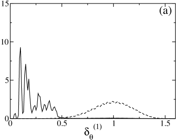
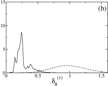
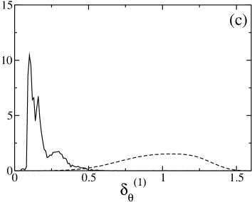
Figure 1: Probability density of angular distances $\delta_{\Theta}^{(1)}$ for all the pairs of minima, $P_{a}$ (dashed line), and for DCP, $P_{c}$ (solid line), for the sequences S0 (a) and S1 (b) and S2 (c).

A qualitatively similar difference between $P$ and $P_{c}$ is observed also for different choices of $q$ as well as for the global distance $\delta_{r}^{(q)}$. In order to identify the most appropriate value of $q$, it is convenient to introduce the integrated fraction $R(\delta)$ of pairs of minima whose distance is smaller than $\delta$

$$R(\delta)=\int_{0}^{\delta}P(x){\rm d}x$$ (5)

and, equivalently,

$$R_{c}(\delta)=\int_{0}^{\delta}P_{c}(x){\rm d}x\,,$$ (6)

relative to DCP. Upon considering $\delta$ as a dummy variable, it is possible to plot $R_{c}$ versus $R$. A fast convergence of $R_{c}$ to 1 means that almost all DCP can be already identified by limiting the search to relatively close pairs of minima. The data plotted in Fig.2a for S1 and $q=1$ indeed reveal such a fast growth of $R_{c}$, that almost $90\%$ of the DCP can be obtained by investigating only $1\%$ of all pairs both by considering the angular $\delta_{\theta}^{(q)}$ and the global $\delta_{r}^{(q)}$ distance. The curves in Fig.2b show that significantly worse performances are obtained when the maximum norm ($q=\infty$) is used to classify the pairs of minima. In order to clarify the role of the parameter $q$, in Figs.3,4, we have plotted $R_{c}$ versus $R$ for different values of this parameter. There we see that, upon decreasing $q$ from $\infty$ down to $1$, $R_{c}$ exhibits an increasingly fast saturation, while the opposite is observed when $q$ is further decreased below $1$. The bad performance observed at high $q$-values has a quite intuitive explanation: in that limit, the norm reduces to the maximum norm and the slow growth of $R_{c}$ tells us that distances between DCP are not uniformly small along all directions: DCP may significantly differ along specific directions in spite of being “on the average” much closer than generic pairs of minima. The relatively bad performance observed for $q\to 0$ has a complementary explanation. In that limit, the average distance is strongly biased by small differences $\delta\theta$ or $\delta r$, whose occasional occurrence may induce to classify as “close”, configurations that are significantly different instead. In all configurations we have investigated, it turns out that $q\approx 1$ is the best compromise between the above two effects. Having established that $q=1$ is the best choice, from now on, we limit ourselves to considering that value and drop the superscript $(1)$ in the definition of the distance.

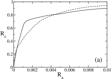
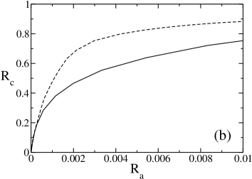
Figure 2: Integrated probability density $R_{c}$ versus $R_{a}$ for the angular $\delta_{\Theta}$ (solid lines) and global $\delta_{r}$ (dashed lines) distances. The data refer to the the sequence S1 and to the absolute value (a) and maximum (b) norm.

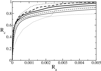
Figure 3: Integrated probability density $R_{c}$ versus $R_{a}$ for the angular distance for various norms for the sequence S0. Contiuous lines correspond to $q<1$ ($q=0.01$, $q=0.2$, $q=0.5$, and $q=0.75$, going from the thinnest to the tickest line, respectively). The dashed line corresponds to $q=1$ (norm of the absolute value). The dotted lines correspond $q>1$ ($q=2$, $q=5$, and $q=\infty$, going from the thickest to the thinnest line, respectively).

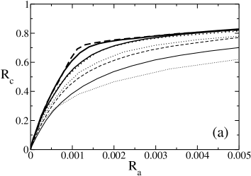
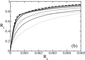
Figure 4: Integrated probability density $R_{c}$ versus $R_{a}$ for the angular distance for various norms for the sequences S1 (a) and S2 (b). The notations are the same as in Fig.3

In practice, since it is eventually necessary to identify a threshold distance $\delta_{\theta}^{\star}$, it is convenient to look also at the dependence of $R_{c}$ on $\delta_{\theta}$ and to introduce

$$\rho(\delta_{\theta})=\frac{R_{c}(\delta_{\theta})}{R(\delta_{\theta})}$$

From Fig. 5, we see that $\delta_{\Theta}^{\star}=0.5$ is a good choice, since $\rho(0.5)\sim{\cal O}(10^{-2})$, while $R_{c}(0.5)\sim 99\%$. Even reducing the threshold value to $\delta_{\theta}^{\star}=0.2$ a large fraction of DCP are still recovered ($R_{c}(0.2)\sim 90\%$).

These results indicate that if one restricts the search of DCP to the set of minima whose distance is smaller than a prescribed threshold $\delta_{\theta}^{\star}$, one can reduce significantly the most time-consuming part of the systematic search algorithm, which amounts to testing whether a generic pair of minima is separated by a single saddle.

Figure 5: The ratio $\rho$ between DCP and all pairs up to distance $\delta_{\Theta}$ (continuous line) compared with $R_{c}(\delta_{\Theta})$ (dashed line) for the three analyzed sequences, S0 (a), S1 (b) and S2 (c).

The drawback is that for any choice of $\delta_{\theta}^{\star}$, those DCP whose mutual distance is anomalously large are going to be missed. In the next Section we analyse the EL with the main goal of concluding whether such a component is of some relevance in the overall reconstruction of the EL.

IV A closer inspection of the Energy Landscape

A faithful reconstruction of the EL requires a sufficiently large database of stationary points, i.e. minima and saddles. The procedure described in the Appendix is quite reliable in this respect, but it is also computationally very time-consuming as already stated. In the previous section we have seen that a large fraction of DCP can be obtained by adopting a suitable metric criterion. However, it is not a priori clear whether the long-distance tail of $P_{c}$ is qualitatively irrelevant too.

In order to shed some light on this question we have divided the minima into “shells”: the $n$–th shell is defined as the collection of all minima which are separated from the NC by at least $n$ saddles. The identification of the minima belonging to each shell can be achieved recursively:

• the 0-th shell coincides with NC;

• a minimum ${\cal C}_{1}$, directly connected to a minimimum ${\cal C}_{2}$ of the $i$-th shell, is identified as part of the $i+1$-st shell if ${\cal C}_{2}$ does not belong to a shell of order $j\leq i$.

In Fig. 6, we report the average value $\bar{\delta}_{\theta}$ of the distance between DCP belonging to consecutive shells for all of the three sequences. This figure indicates that the interminimum distance grows in the vicinity of the NC. The average distance $\langle\delta_{\theta}\rangle$ between DCP lying inside the same shell exhibits the same behaviour. Finally, this rarefied density of minima in the vicinity of the NC is confirmed also by plotting the mutual distance versus the actual distance from the NC. In this case, in order to smoothen the wild pair-to-pair fluctuations, a coarse-graining has been performed by averaging over bins of widht 0.01 along the $\delta_{\theta}$ axis (see Fig. 7).

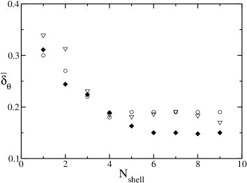
Figure 6: Average connection length between the minima of the $i$-th and $i-1$-th shell for the three sequences S0 (triangles), S1 (circles) and S2 (filled diamonds).

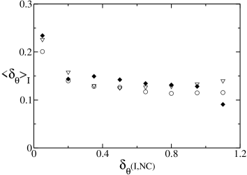
Figure 7: The average distance of minima from their connected set versus their distance from the NC for the sequence S0 (triangles), S1 (circles) and S2 (filled diamonds). The data are averaged also over intervals of length $I=0.01$ along the horizontal axis.

Altogether, the significative increase of the average distance close to the NV indicates that some of the DCP that are missed by the metric criterion discussed in previous section lie in the most relevant region for the characterization of the folding/unfolding processes. However, considering the limited number of minima in the NV, such a difficulty can be easily overcome by complementing the overall application of the metric criterion with an extensive comparison of such minima with all configurations in the database: the additional cost in terms of the computing time is indeed a minor one.

The increased distance between neighbouring minima hints at possibly deeper valleys and is, in turn, suggestive of the presence of a funnel in the EL, a structure that is typically expected to appear in true proteins funnel . However, we find this scenario in all of the three sequences analyzed in this paper, including the homopolymer S0 which cannot be certainly considered a reasonable model for a protein. In order to further clarify this point, we have computed the escape rates from the single valleys. Given any two directly connected minima ${\cal C}_{1}$ and ${\cal C}_{2}$ characterized by the potential energies $V_{1}$ and $V_{2}$ ($V_{1}\leq V_{2}$), the escape rate from the minimum ${\cal C}=\{{\cal C}_{1},{\cal C}_{2}\}$ through the saddle ${\cal C}_{s}$ (with potential energy $V_{s}$) is given by

$$\Gamma_{\cal C}=\frac{\omega_{\parallel}}{\pi\gamma}\frac{\prod_{i=1}^{L^{\prime}}\omega_{\cal C}^{(i)}}{\prod_{i=1}^{L^{\prime}-1}\omega_{\perp}^{(i)}}\exp\left\{-\frac{W_{\cal C}}{k_{B}T}\right\}\quad.$$ (7)

This formula, proposed by Langer langer ; review , is obtained by considering the harmonic approximation of the potential in the vicinity of ${\cal C}_{1}$, ${\cal C}_{2}$, and ${\cal C}_{s}$. The $\omega_{\cal C}^{(i)}$’s are the $L^{\prime}=2L-3$ non zero frequencies of the minimum $\cal C$ ($\omega_{\cal C}^{(i)}=\sqrt{-\Lambda_{\cal C}^{(i)}}$, where $\Lambda_{\cal C}^{(i)}$ is the $i$-th negative eigenvalue of the Hessian of the potential energy $V$). Analogously, $\omega_{\perp}^{(i)}$’s are the $L^{\prime}-1$ non zero frequencies of the saddle (those corresponding to the stable directions), while $\omega_{\parallel}$ is associated with the only expanding direction. Finally, $\gamma$ is the dissipation rate nota1 , while the Arrhenius exponential factor depends on the height of the barrier, $W_{\cal C}=V_{s}-V_{1,2}$, normalized to the reduced temperature $K_{B}T$, $K_{B}$ being the Boltzmann constant.

The above expression has been shown to reproduce reasonably well the numerically obtained escape rates for heteropolymers in 2d at moderate temperatures for $T<\approx T_{\theta}$ tap . Accordingly, in that regime, both the folding and the unfolding dynamics towards and from the NC are driven by thermal activation processes, which determine the transitions between DCP. Small $\Gamma$-values suggest that the heteropolymer may be trapped into some local valley of the EL, far from the NC. Eq. (7) shows explicitly that in high–dimensional spaces, the escape rate does not simply depend on the energy barriers but also on entropic factors, which depend on geometrical features of basins of attractions of the stationary configurations in the EL.

In Fig. 8 we have plotted the rates $\Gamma_{\cal C}$ as a function of $\delta_{\theta}$ for the three sequences at $T=T_{f}$ and $\gamma=1$ (since past simulations indicate that the effective value of $\gamma$ is the same at least in the whole NV, there is no need to know it when a comparative analysis is being carried out). There we notice a striking difference between S0 and S1 at large distances: actually the escape rates of S0 are two orders of magnitude smaller than those of S1. Moreover, $\Gamma_{{\cal C}_{2}}\sim{\cal O}(1)$ almost in the whole range of distances $\delta_{\theta}$ for S1, indicating that no trapping is expected in the shallower minima, while it exhibits an almost exponential decrease for S0. An intermediate situation is observed for S2 at large distances. As a result, we see that a true funnel-like structure is markedly present only in the EL of the sequence S1, that was indeed already identified as a good folder by looking at different indicators irback1 ; tlp .

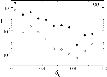
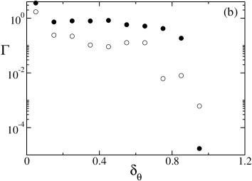
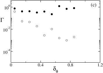
Figure 8: Escape rates (7) versus the angular distance $\delta_{\Theta}$ for each DCP for sequence S0 (a) and S1 (b) and S2 (c) at a temperature $T=T_{f}$ (namely, $T_{f}=0.044$ for S0 and S2, $T_{f}=0.061$ for S1). The filled circles refer to the transition rates $\Gamma_{{\cal C}_{1}}$, while the empty circles to $\Gamma_{{\cal C}_{2}}$.

V Conclusions and perspectives

In this paper we have analyzed the structure of the energy landscape (EL) of a 2d off-lattice model of a polypeptidic chain and found that the relative closeness between neighbouring minima can be exploited to implement an effective algorithm to identify directly connected minima. In order to put the analysis on firm quantitative grounds, we have tested several definitions of distance between configurations, finding that the best performances are obtained for the angular distance $\delta_{\theta}^{(1)}$ (see Eq. (3)). In fact, the $\delta_{\theta}^{(1)}$ distances corresponding to DCP are more sharply concentrated at small values than for all other definitions of distances. In particular, we have found that restricting the systematic search to all pairs of minima whose distance is smaller than $\delta_{\theta}^{(1)\star}=0.5$, one can recover almost $99\%$ of all DCP. The drawback of this approach is that a tiny fraction of DCP is unavoidably missed, but the consequences are not a priori clear. Since our analysis of the native valley has shown that minima are more rarefied in the vicinity of the native configuration (see Fig. 7), we conclude that it is wise to complement the above metric criterion with an extensive search limited to the minima of the native valley. It is now important to verify to what extent such a scenario extends to more realistic 3D systems, where the implementation of effective algorithms to reconstruct the EL is even more crucial than in 2D. Furthermore, important hints about the true relevance of missing links in a connectivity graph will come after imposing a dynamics on the graph itself by adding the activation rates $\Gamma$ relative to the transitions between directly connected minima. By comparing the resulting evolution with that of the original system one can in particular determine the minimal fraction of DCP that is necessary to identify for a meaningful reconstruction of the folding process.

Finally, in order to test how the observed rarefied density of minima in the vicinity of the NC is connected to the presence of a true funnel-like structure, we have computed the activation rate $\Gamma$ inside the NV. It turns out that moving away from the NC, while in the homopolymer $\Gamma$ decreases very rapidly, it stays almost constant in the sequence S1, previously identified as a good foolder by other means. This is a clear indication that the homopolymer can be trapped in several minima far from the minimal energy state, while an accessible native valley does exist for S1.

• Given two minima ${\cal C}_{1}$ and ${\cal C}_{2}$ and two configurations ${\cal P}_{1}$ and ${\cal P}_{2}$ belonging to their basins of attraction, one wants to determine two configurations ${\cal Q}_{1}$ and ${\cal Q}_{2}$ on the segment ${\cal P}_{1}{\cal P}_{2}$ arbitrarily close to the ridge dividing the two basins and lying on its opposite sides;

• given ${\cal Q}_{1}$ and ${\cal Q}_{2}$, as defined above, one wants to apply an iterative procedure, leading the two points to converge on the saddle.

The procedure is here described in more details:

1. given ${\cal Q}_{1}={\cal P}_{1}$ and ${\cal Q}_{2}={\cal P}_{2}$, an intermediate configuration ${\cal C}$ is defined, by setting its bond angles equal to the average of the corresponding angles of ${\cal Q}_{1}$ and ${\cal Q}_{2}$;

2. a steepest descent procedure is applied to ${\cal C}$ until a minimum ${\cal C}_{m}$ is reached;

3. 1. if ${\cal C}_{m}$ coincides with ${\cal C}_{1}$ (${\cal C}_{2}$), we replace ${\cal Q}_{1}$ (${\cal Q}_{2}$) with ${\cal C}$ and repeat the step (2) until the euclidean distance $d_{E}({\cal Q}_{1},{\cal Q}_{2})$ between ${\cal Q}_{1}$ and ${\cal Q}_{2}$ becomes smaller than a given threshold $\delta$;

   2. if ${\cal C}_{m}$ differs from both ${\cal C}_{1}$ and ${\cal C}_{2}$, we assume that the basins of attraction of the two minima are not directly connected (i.e., ${\cal C}_{1}$ and ${\cal C}_{2}$ are not neighbors) and ${\cal C}_{m}$ is added to the minima database, provided it is not already included;

   3. if $d_{E}({\cal Q}_{1},{\cal Q}_{2})<\delta$, we conclude they are close enough to the ridge (i.e. the stable manifold separating the basins of attraction of ${\cal C}_{1}$ and ${\cal C}_{2}$) and pass to item (4);

4. we let ${\cal Q}_{1}$ and ${\cal Q}_{2}$ evolve in time according to a steepest descent relaxation until $d_{E}({\cal Q}_{1}(t),{\cal Q}_{2}(t))$ becomes larger than $\delta$ and go back to (1), identifying ${\cal P}_{1}$ with ${\cal Q}_{1}(t)$ and ${\cal P}_{2}$ with ${\cal Q}_{2}(t)$;

5. when, during the steepest descent, the gradient of the potential both in ${\cal Q}_{1}$ and ${\cal Q}_{2}$ becomes smaller than another given threshold, we assume ${\cal Q}_{1}$ and ${\cal Q}_{2}$ to be close enough to a first order saddle and refine the configuration by means of a Newton’s algorithm.

It must be stressed that this algorithm not only allows to find first order saddles but also enriches the number of known minima. The saddle-searching strategy here proposed can then be viewed as an “all purpose” method suitable for a complete exploration of all the features of the EL relevant for protein dynamics.

The data reported in this paper were obtained by applying the algorithm to an initial database of minima determined by the method described in Ref. tap . It amounts to performing a high-temperature (typically above $T_{f}$) Langevin dynamics, when the system is expected to visit a large portion of the accessible phase space. The resulting trajectory is then sampled to pinpoint a series of configurations, which are afterwards relaxed according to a steepest descent dynamics and finally refined by means of a standard Newton’s method. This procedure was used for identifying a small database of 50-100 collapsed states for each of the three sequences described in section II.

All possible pairs in these initial minima databases were then searched for DCP by means of our saddle-finding algorithm. The new minima found during each run of the algorithm on all possible pairs were stored in the database to be investigated in successive runs. Actually the number of pairs of minima grows much faster than the number of pairs investigated, thus making impossible a complete analysis. The number of minima and saddles that were identified after three runs is reported in Table 1.

In order to perform a complete search of all DCP at least in a restricted set of minima, we have selected all configurations of energy lower than $V_{f}=V_{0}+LT_{f}$. In this restricted database all pairs of minima characterized by an angular distance smaller than $0.5$ where investigated. The total number of saddles found by this procedure is reported in Table 1.

Table 1: Number of minima in the whole database and in the first and second shell. Number of investigated pairs and number of DCP found. Data have been reported for all the three examined sequences.

	S0	S1	S2
Total number of minima	$2.3\times 10^{5}$	$7.2\times 10^{4}$	$6.4\times 10^{4}$
Number of minima in the 1st shell	64	50	49
Number of minima in the 2nd shell	1,181	465	348
Number of minima below $T_{f}$	66,470	5,883	8,670
Number of investigated pairs	$9.1\times 10^{6}$	$0.94\times 10^{6}$	$1.3\times 10^{6}$
Number of connected pairs	84,990	10,470	14,356

References

- (1) D.J. Wales, Energy Landscapes, Cambridge University Press, Cambridge, 2003.
- (2) F.H. Stillinger and T.A. Weber, Science 225 (1984) 983.
- (3) S. Sastry, P.G. Debenedetti, and F.H. Stillinger, Nature 393 (1998) 554.
- (4) L. Angelani, R. Di Leonardo, G. Ruocco, A. Scala, and F. Sciortino, Phys. Rev. Lett. 85 (2000) 5356.
- (5) S.V. Krivov and M. Karplus, J. Chem. Phys 117 (2002) 10894.
- (6) D.A. Evans and D.J. Wales, J. Chem. Phys 118 (2003) 3891.
- (7) A. Baumketner, J.-E. Shea, and Y. Hiwatari, Phys. Rev. E 67 (2003) 011912.
- (8) P.E. Leopold, M. Montal, and J.N. Onuchic, Proc. Natl. Acad. Sci. USA 89 (1992) 8721.
- (9) A. Torcini, R. Livi, and A. Politi, J. Biol. Phys. 27 (2001) 181.
- (10) L. Bongini, R. Livi, A. Politi, and A. Torcini, Phys. Rev. E 68 (2003) 061111.
- (11) F.H. Stillinger, T.H. Gordon, and C.L. Hirshfeld, Phys. Rev. E 48 (1993) 1469.
- (12) E. Marinari, and G. Parisi, Europhys. Lett. 19 (1992) 451.
- (13) A. Irbäck and F. Potthast, J. Chem. Phys. 103 (1995) 10298.
- (14) A. Irbäck, C. Peterson, and F. Potthast, Phys. Rev. E 55 (1997) 860.
- (15) P.G. De Gennes, Scaling Concepts in Polymer Physics Cornell University Press, 1979, New York.
- (16) T. Veitshans, D. Klimov, and D. Thirumalai, Folding & Design 2 (1997) 1.
- (17) J.S. Langer, Ann. Phys. 54 (1969) 258
- (18) P. Hänggi, P. Talkner, and M. Borkovec, Rev. Mod. Phys. 62 (1990) 251.
- (19) This is a free parameter, which has to be fixed according to some physical criterion.