Effects of an external magnetic field on the gaps and quantum corrections in an ordered Heisenberg antiferromagnet with Dzyaloshinskii-Moriya anisotropy

Abstract

We study the effects of external magnetic field on the properties of an ordered Heisenberg antiferromagnet with the Dzyaloshinskii-Moriya (DM) interaction. Using the spin-wave theory quantum correction to the energy, on-site magnetization, and uniform magnetization are calculated as a function of the field $H$ and the DM anisotropy constant $D$. It is shown that the spin-wave excitations exhibit an unusual field-evolution of the gaps. This leads to various non-analytic dependencies of the quantum corrections on $H$ and $D$. It is also demonstrated that, quite generally, the DM interaction suppresses quantum fluctuations, thus driving the system to a more classical ground state. Most of the discussion is devoted to the spin-$S$, two-dimensional square lattice antiferromagnet, whose $S=\frac{1}{2}$ case is closely realized in K₂V₃O₈ where at $H=0$ the DM anisotropy is hidden by the easy-axis anisotropy but is revealed in a finite field. The theoretical results for the field-dependence of the spin-excitation gaps in this material are presented and the implications for other systems are discussed.

I Introduction

The studies of quantum antiferromagnets (AFs) in external magnetic field attract significant attention because these systems exhibit a variety of unusual quantum-mechanical phenomena of general interest. The modern high magnetic field technology, materials’ synthesis, and experimental probes allow precise measurements in the regime of the field strength comparable to the characteristic exchange constant of a system. This has made possible the observations of condensation of triplet excitations in a variety of chain, ladder, and weakly-coupled dimer compounds,Zheludev ; S=1 ; BEC magnetization plateaux in frustrated magnets,plato and other new effects.Dender ; Kakurai It turned out that in many cases experimental data deviate significantly from the theoretical predictions based on the pure isotropic Heisenberg model in external field.Dender ; Sushkov ; S=1a Such deviations are due to anisotropies, most notably the Dzyaloshinskii-Moriya (DM) anisotropy, which are usually small and often neglected from zero-field considerations. Not only such anisotropies can induce qualitatively new effects, but also the strength of such effects seems to be significantly amplified by an external field. In particular, in the one-dimensional (1D) spin-$\frac{1}{2}$ chains with the DM interaction spin excitation spectrum exhibits a gap $\Delta\propto(DH)^{2/3}$ in contrast with the pure Heisenberg case where the spectrum remains gapless.Dender ; Affleck Thus, while usually treated as an insignificant contamination of the problem, the DM interaction can give rise to an interesting phenomena on its own.

In the case of the 1D spin-chains an unusual field-dependence of the gap has been first documented experimentallyDender and has received a theoretical explanation soon after that.Affleck ; YuLu For the higher-dimensional cases there is a recent theoretical expectationAffleck ; Sato ; Mila that the field-dependence of one of the gaps should be $\Delta\propto(DH)^{1/2}$. However, such a behavior has not been observed in any known system yet. There is also a disagreement between the recent theoretical worksSato ; Mila in the low-field regime with the earlier low-field studies of the Heisenberg$+$DM problem.Pinkus ; footnote1 ; Trugman The latter works predict a non-zero gap and also weak ferromagnetismDzyaloshinskii in zero field, while the former do not. We will show below that this discrepancy comes from the higher-order contributions, which yet result in the effects of order ${\cal O}(D)$ in the excitation gap and spin canting angle. We will also show that in a realistic system the low-field behavior can be more delicate. The field-dependence of the gap, quite generally, takes the form $\Delta\propto\sqrt{D(H-H^{*})}$, where $H^{*}\sim D$ can be both positive and negative depending on the system. This clarifies theoretical expectation for experiments.

Furthermore, most of the studies have excluded from consideration the quantum effects associated with the DM interaction. The generic question is: does the DM interaction enhance or suppress quantum fluctuations? This is important for the systems close to the spin-liquid state, such as triangular lattice AF Cs₂CuCl₄ where the DM term is significant,Coldea ; Veillette ; footnote2 and also for the frustrated spin systems where quantum effects may help to select the ground state.Kotov ; Canals

In this work we study the excitation spectrum and various $T=0$ static properties of the square lattice, spin-$S$ Heisenberg model with the DM interaction. This is the simplest case of a higher-dimensional system in which generic trends of the mutual effect of the DM interaction, external field, and quantum fluctuations on the properties of an ordered AF can be studied. This choice is also motivated, in part, by the recent experiments in K₂V₃O₈, a 2D, $S=\frac{1}{2}$ AF, which demonstrates an unusual spin-reorientation transition in a small field.Lumsden This effect has been understood as resulting from an interplay of the DM and easy-axis anisotropies.

Altogether, the purpose of this work is threefold. First, to reconcile the earlier low-field and recent high-field theoretical studies of the Heisenberg$+$DM$+$field problem. Second, to study the dependence of the quantum corrections on the DM interaction. Third, to analyze an experimental system to which these results can be applied.

We find that the gap in one of the magnon branches shows the following behavior when ${\bf H}\perp{\bf D}$: $\Delta_{\pi\pi}=D$ in $H=0$ field, $\Delta_{\pi\pi}=\sqrt{D}$ for $H\simeq 0.7H_{s}$, and $\Delta_{\pi\pi}=\sqrt{3}D^{2/3}$ for $H=H_{s}$, where $H_{s}$ is the saturation field and the energy units $=4SJ$ are used. These findings are in agreement with the other works.Pinkus ; Sato ; Mila We also show that, for the fields $0<H\lesssim H_{s}$, the DM interaction leads to the suppression of the quantum fluctuations. The dependence of the quantum corrections on $D$ for various quantities is often non-analytic. It is only in the regime of the field close to the saturation, $H\sim H_{s}$, where the DM term enhances quantum fluctuations, effectively leading to a proliferation of the quantum effects into the classical saturated phase ($H>H_{s}$). We also show that some quantum corrections are singular in the limit of both $H$ and $D$ going to zero, namely $\lim_{H\rightarrow 0}\lim_{D\rightarrow 0}\neq\lim_{D\rightarrow 0}\lim_{H\rightarrow 0}$. We demonstrate that K₂V₃O₈ is an excellent candidate for the observation of the unusual field-dependence of the gap, characteristic to the 2D and 3D AFs. In fact, an additional easy-axis anisotropy helps to switch between the Ising-like and easy-plane behavior in this system, making it potentially possible to observe a non-analytic $\Delta\propto\sqrt{H-H^{*}}$ behavior of the gap.footnote3

The paper is organized as follows. In Sec. II we describe the technical details, derive the spin-excitation spectrum, and present the results for the quantum corrections to various quantities in different field regimes. In Sec. III we give a quantitative discussion of the excitation spectrum in K₂V₃O₈. We conclude by Sec. IV which contains a brief discussion of our results.

II Model, spectrum, and quantum corrections

As is mentioned in Introduction, we would like to consider the simplest possible case of an ordered AF with the DM anisotropy in an external field, which would allow to investigate the role of quantum corrections in it. We therefore study the spin-$S$, nearest-neighbor Heisenberg model on a square lattice with the DM interaction:

$${\cal H}=\sum_{\langle ij\rangle}\bigg{(}J{\bf S}_{i}\cdot{\bf S}_{j}+{\bf D}_{ij}\cdot({\bf S}_{i}\times{\bf S}_{j})\bigg{)}-\sum_{i}{\bf H}\cdot{\bf S}_{i},$$ (1)

$\langle ij\rangle$ denotes summation over bonds and ${\bf H}$ is the magnetic field in the energy units ($g\mu_{B}=1$). The direction of the (staggered) DM vector will be chosen along the $z$-axis, ${\bf D}_{ij}=(-1)^{i}(0,0,D)$. Aside from being the simplest and the most commonSato ; Veillette choice, this Hamiltonian also corresponds closely to K₂V₃O₈.footnote4 We would like to note that, generally, this form of the Hamiltonian is incomplete, because, as noted in Refs. Shekhtman1, ; Shekhtman2, ; Yildrim, , the same microscopic processes that generate the DM cross-product term also yield the higher-order ${\cal O}(D^{2})$ terms, which contribute to some observables on equal footing. Without going into much details we refer to the same worksShekhtman1 ; Shekhtman2 ; Yildrim which show that these additional terms can be cast in the form of an easy-axis anisotropy with the “easy” axis along the ${\bf D}$-vector, also the case realized in K₂V₃O₈. Quite generally, the DM constant $D$ and the easy-axis anisotropy constant $E$ are not related to each other in a straightforward way and thus can be treated as phenomenological parameters. Therefore, in the following we would like to concentrate on the most commonly used Hamiltonian (1) which only contains the cross-product DM-term and will consider the effect of the easy-axis anisotropy later in the context of K₂V₃O₈, Sec. III. It is convenient to use units $J=1$ in Eq. (1) and this convention is used throughout the paper unless noted otherwise.

II.1 Classical limit

It is important to discuss the classical limit of the model (1) first, as for the consideration of the excitation spectrum the quantization axes for spins will be chosen along their classical directions. The effect of the DM interaction is twofold: it makes energetically favorable for the spins to stay in the plane perpendicular to the direction of ${\bf D}$ and, without the $J$-term, it would make the spins in different sublattices to be under an $\alpha=\pi/2$ angle to each other (in the notations of Fig. 1 that corresponds to the angle $\varphi=(\pi-\alpha)/2=\pi/4$). While the former trend can only be hindered by additional anisotropies (see next Section) the latter always competes with the much larger Heisenberg term which prefers the spins to stay antiparallel. Thus, at $H=0$ in the ground state of the model (1) spins lie in the $x-y$ plane and are canted towards each other. According to Fig. 1 this configuration has a finite angle $\varphi(H=0)=\frac{1}{2}\tan^{-1}D$ resulting in a non-zero uniform magnetization $M=S\sin\varphi\simeq SD/2$ (per spin). Therefore, the $H=0$ limit of the model (1) exhibits an effective easy-plane anisotropy and a weak ferromagnetism, a phenomenon the DM interaction was originally proposed for.Dzyaloshinskii

It is clear now that there are two distinct choices for the direction of the external field: one is along the DM vector, ${\bf H}\parallel z$, and the other one is perpendicular to it, ${\bf H}\perp z$. We will be mostly concerned with the latter case of the in-plane field as it leads to most non-trivial results and will only briefly discuss the former. From the symmetry point of view these two cases are clearly distinct because the symmetry is lowered by the DM interaction already in zero field from the full rotational $O(3)$ symmetry to the easy-plane $O(2)$ symmetry. Then the field along the $z$-axis will only cant the spins towards itself without affecting the freedom of choice of the spontaneous in-plane spin direction, thus leaving $O(2)$ intact. On the other hand, the in-plane field will break the remaining continuous $O(2)$ symmetry and “pin” the spins’ direction in the plane.

Canting angles at $D=0$.   Since the magnitude of the DM interaction is generally small one may wonder how much difference its presence makes for the ground state of the model (1) for the finite, and not necessarily small, values of $H$. While we will address this issue in detail below it is instructive to consider the spin configuration when $D=0$. If we neglect the DM interaction in (1) the only effect of the external magnetic field is to induce a finite uniform magnetization by canting spins towards the field. The canting angle is $\varphi_{0}=\sin^{-1}(H/8S)$ and the spins become fully polarized in the saturation field $H_{s}=8S$ (where $8=2z$, $z=4$ is the coordination number for the square lattice).

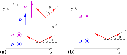
Figure 1: (Color online) (a) ${\bf H}\|{\bf D}\|z$ configuration. The canting angle $\varphi$ in the $x-y$ plane is induced by the DM interaction and does not depend on the field. The canting angle $\theta$ towards the field ($z$-axis) is given by Eq. (3). (b) ${\bf H}\perp{\bf D}$ configuration. The canting angle $\varphi$ is given by Eq. (5).

II.1.1 Out-of-plane field.

We now consider the field-dependence of the canting angles in the presence of the DM interaction. If the field is perpendicular to the $x-y$ plane the canting induced by the $D$-term and the one induced by the field lie in the orthogonal planes, see Fig. 1(a). Therefore, one should expect the DM-induced in-plane canting angle $\varphi$ to be independent of the field. Using the angle notations of Fig. 1(a) the classical energy of the model Eq. (1) can be written as:

$$\frac{E_{cl}}{2NS^{2}}=1-\sin^{2}\theta\left(2\cos^{2}\varphi+D\sin 2\varphi\right)-\frac{H}{2S}\cos\theta\ ,$$ (2)

minimizing which gives the canting angles, $N$ is the number of lattice sites. As expected, $\varphi=\frac{1}{2}\tan^{-1}D$ is independent of the field and the field-induced out-of-plane canting angle should be found from:

$$\cos\theta=\frac{H}{8S}\ \frac{2}{1+\sqrt{1+D^{2}}}\ .$$ (3)

Thus, the only effect of the small DM interaction for the case of ${\bf H}\|{\bf D}$ is the slight change of the saturation field from $H_{s}=8S$ to $H_{s}^{\|}=4S\left(1+\sqrt{1+D^{2}}\right)$.

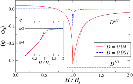
Figure 2: (Color online) The difference of the in-plane canting angle $\varphi$ and its $D=0$ limit $\varphi_{0}$ v.s. field in the ${\bf H}\perp{\bf D}$ configuration for two representative values of $D=0.001$ (dashed lines) and $D=0.04$ (solid lines), $D$ is in units of $J$. Inset: the canting angle $\varphi$ v.s. field. The asymptotic behavior of $\varphi-\varphi_{0}=-DH_{s}/2(H-H_{s})$ is shown by the dotted line. $D^{1/3}$ values for both choices of $D$ are shown by the horizontal dashed lines.

II.1.2 In-plane field.

For the in-plane field the changes for the canting angle are less trivial. The spins are in the $x-y$ plane, see Fig. 1(b). From minimizing the classical energy:

$$\frac{E_{cl}}{2NS^{2}}=-\cos 2\varphi-D\sin 2\varphi-\frac{H}{2S}\sin\varphi\ ,$$ (4)

the canting angle obeys the following equation:

$$\sin\varphi-\frac{D}{2}\frac{\cos 2\varphi}{\cos\varphi}=\frac{H}{8S}.$$ (5)

Without the DM interaction Eq. (5) yields a familiar $H$-dependence of the canting angle: $\varphi_{0}=\sin^{-1}(H/8S)$ (0 in the subscript refers to $D=0$). To demonstrate the effect of the DM interaction on the canting angle in the ${\bf H}\perp{\bf D}$ case we plot the difference of $(\varphi-\varphi_{0})$ v.s. field for two representative values of $D$ in Fig. 2. One can see that the difference is $D/2$ for small field and it vanishes for the field $H\simeq 0.707H_{s}$. This field makes the angle between the spins to be $\pi/4$ for any value of $D$. Thus, the DM-term in the energy is always fully minimized for such a field. The most striking feature in this plot is the sharp singularity at $H=H_{s}$. This is due to the fact that the $D=0$ canting angle $\varphi_{0}$ exhibits a kink at $H_{s}$ where it reaches the maximal value $\pi/2$. In contrast, the field-dependence of the canting angle $\varphi$ is smooth through the saturation field, as shown in the inset of Fig. 2. In fact, the spins never fully saturate, only as $H\rightarrow\infty$. The asymptotic behavior of the angle is: $\varphi-\pi/2=-DH_{s}/2(H-H_{s})$, which is shown in Fig. 2 by the dotted line. Therefore, the saturation field formally ceases to exist for the ${\bf H}\perp{\bf D}$ case. In the rest of the paper we refer to the “bare” ($D=0$) value $H_{s}=8S$ as to the value of the saturation field. It is interesting to note that the magnitude of the deviation of the canting angle from its $D=0$ value is quite significant close to the saturation field. Taking $H=H_{s}$ and assuming $D\ll 1$ one can find from Eq. (5) that $\cos\varphi\simeq\pi/2-\varphi\simeq D^{1/3}$, a value which is not necessarily small even if $D$ itself is reasonably small. The $D^{1/3}$ values for the choices of $D$ are shown in Fig. 2 by the horizontal dashed lines.

II.2 Spectrum and gaps

Technical approach.   To apply the spin-wave theory to the model (1) we follow the general prescription of Ref. Zhitomirsky, . Namely, the rotating local reference frame for each sublattice is introduced in which the quantization axis $z_{0}$ is directed along the classical spin direction. In such a local frame the standard bosonic representation for the spin operators is used:

$$S^{z_{0}}=S-a^{\dagger}a,$$

$$S^{x_{0}}=\frac{S^{+}+S^{-}}{2}=\sqrt{\frac{S}{2}}(a+a^{\dagger}),$$ (6)

$$S^{y_{0}}=\frac{S^{+}-S^{-}}{2i}=-i\sqrt{\frac{S}{2}}(a-a^{\dagger}),$$

where we omit higher-order boson terms from $S^{\pm}$ thus restricting ourselves to the linear spin-wave approximation. Higher-order, as usual, means both the higher number of boson operators and the higher powers of $1/S$. Then one needs a transformation of the spin components from the local reference frame to the laboratory reference frame. Such transformations are again based on the classical considerations of the canting angles similar to the ones given in Sec. II.1, and they depend on the relative direction of the field, anisotropies, etc. To give a specific example we provide here such a transformation for the ${\bf H}\perp{\bf D}$ configuration for the vectors ${\bf D}\|z$ and ${\bf H}\|y$, see Fig. 1(b):

$$S^{x}_{i}=-S^{x_{0}}_{i}\sin\varphi+S^{z_{0}}_{i}(-1)^{i}\cos\varphi$$

$$S^{y}_{i}=S^{z_{0}}_{i}\sin\varphi+S^{x_{0}}_{i}(-1)^{i}\cos\varphi$$ (7)

$$S^{z}_{i}=S^{y_{0}}_{i}\ .$$

Using relations of that type and representation (II.2) one can rewrite the Hamiltonian (1) in the form:

$${\cal H}=E_{cl}+{\cal H}_{LSWT}+\dots\ ,$$ (8)

where $E_{cl}$ is the classical energy discussed above, the ellipsis stands for the higher-order terms, and the spin-wave Hamiltonian can be written in the general form:

$${\cal H}_{LSWT}=4S\sum_{\bf k}\bigg{(}\Big{(}C_{1}+C_{2}\gamma_{\bf k}\Big{)}a_{\bf k}^{\dagger}a_{\bf k}^{\phantom{{\dagger}}}$$ (9)

$$\phantom{{\cal H}_{LSWT}=4SJ\sum_{\bf k}\bigg{(}}+\frac{C_{3}\gamma_{\bf k}}{2}\left(a_{\bf k}^{\dagger}a_{-{\bf k}}^{{\dagger}}+a_{\bf k}a_{-{\bf k}}\right)\bigg{)}\ ,$$

where $\gamma_{\bf k}=(\cos k_{x}+\cos k_{y})/2$ and the summation over ${\bf k}$ is over the full Brillouin zone (BZ). All the coefficients $C_{i}$ are the functions of the field and anisotropies. As is noted in Ref. Zhitomirsky, , the minimization of the classical energy ensures the absence of the terms linear in $a$, or $a^{\dagger}$ in the expansion of the Hamiltonian (8). Then, the spin-wave Hamiltonian is readily diagonalized by the Bogolyubov transformation and takes the form:

$${\cal H}_{LSWT}=\delta E+\sum_{\bf k}\omega_{\bf k}\alpha_{\bf k}^{\dagger}\alpha_{\bf k}^{\phantom{{\dagger}}}\ ,$$ (10)

where the magnon energy is

$$\omega_{\bf k}=4S\sqrt{\Big{(}C_{1}+C_{2}\gamma_{\bf k}\Big{)}^{2}-C_{3}^{2}\gamma^{2}_{\bf k}}\ ,$$ (11)

and

$$\delta E=\frac{1}{2}\sum_{\bf k}\Big{(}\omega_{\bf k}-4SC_{1}\Big{)}\ .$$ (12)

As an example of the use of such a procedure, one can neglect the DM-term for a moment and, after some algebra, obtain: $C_{1}=1$, $C_{2,3}=(-\cos 2\varphi_{0}\pm 1)/2$. This leads to the following expression for the spin-wave spectrum:

$$\omega_{\bf k}^{D=0}=4S\sqrt{(1+\gamma_{\bf k})(1-\cos 2\varphi_{0}\gamma_{\bf k})}\ ,$$ (13)

where $\cos 2\varphi_{0}=1-2(H/H_{s})^{2}$, in agreement with the results of Ref. Zhitomirsky, .

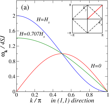
Figure 3: (Color online) Linear spin-wave result, Eq. (13), for the magnon spectrum in a field ($D=0$), for $H=0$, $H=H_{s}/\sqrt{2}$, and $H=H_{s}$ along the main diagonal of the BZ. Inset: full BZ with the direction of the cut. Magnetic BZ is shown by the dashed diamond.

General features of the spectrum.    Before we discuss the details of the gaps’ dependence on both the field and the DM interaction, we would like to outline the broad features of the spin-wave spectrum. Our Fig. 3 shows the $D=0$ spectrum given by Eq. (13) along the main diagonal of the Brillouin zone (see inset) for three representative values of the field. In the $H=0$ case the spectrum has two gapless modes, at $(0,0)$ and $(\pi,\pi)$. In the field one of the modes develops a gap, $\Delta_{00}\equiv H$, which is strictly equal to the value of the field. This mode corresponds to the uniform precession of the field-induced magnetization about the field direction.ZhCh The other mode must remain gapless as it corresponds to the Goldstone mode related to the spontaneous breaking of the remaining $O(2)$ symmetry of the spins in the plane perpendicular to the field.

Two remarks are in order. First, while it is convenient to use the “full” BZ language here with a single magnon branch, one can employ an equivalent picture of two magnon branches within the magnetic BZ (shown in the inset of Fig. 3 by the dashed diamond). The neutron scattering will observe these branches near the $(\pi,\pi)$-point in the different components of the structure factor: ${\cal S}^{\pm}\propto\delta(\omega-\omega_{\bf k})$ and ${\cal S}^{zz}\propto\delta(\omega-\omega_{\bf k-(\pi,\pi)})$, see Ref. ZhCh, . Second, we neglect the higher-order non-linear terms in the spin-wave Hamiltonian. While they do not change most of the results qualitatively, in the fields close to the saturation they induce an instability of the single-magnon branch towards decays into a two-magnon continuum.ZhCh Since such an instability does not concern the ${\bf k}=(0,0)$ and ${\bf k}=(\pi,\pi)$ modes we do not take this effect into account in this work.footnote5

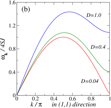
Figure 4: (Color online) Linear spin-wave result, Eq. (14), for the magnon spectrum in zero field for $D=0.04$, $D=0.4$, and $D=1.0$ along the main diagonal of the BZ.

Another general feature of the spin-wave spectrum behavior can be studied by considering the case $H=0$ and $D\neq 0$. Using Eqs. (5), (II.2), and (9) one obtains $C_{1}=\sqrt{1+D^{2}}$, $C_{2,3}=(-\sqrt{1+D^{2}}\pm 1)/2$, which gives:

$$\omega_{\bf k}^{H=0}=4S\sqrt{1+D^{2}}\ \sqrt{(1-\gamma_{\bf k})\left(1+\frac{\gamma_{\bf k}}{\sqrt{1+D^{2}}}\right)}\ .$$ (14)

This spectrum is plotted in Fig. 4 for three different values of $D$. Again, one of the modes is gapless due to the $O(2)$ symmetry, which is now related to the spontaneous choice of the direction of the DM-induced ferromagnetic magnetization vector. The gap in the other mode is $\Delta_{\pi\pi}\simeq 4SD$ for small $D$. These results are very similar to the ones obtained in Ref. Trugman, in the context of La₂CuO₄.

II.2.1 Out-of-plane field.

Having outlined the general trends of the spin-wave spectrum behavior we return to the original problem of the DM interaction in a field. We first consider ${\bf H}\|{\bf D}\|z$ configuration. Recalling our discussion about the canting angles for this case in Sec. II.1.1, and using Eq. (3), after some algebra one obtains:

$$C_{1}=C_{2}+C_{3}=\sqrt{1+D^{2}}\ ,$$ (15)

$$C_{2}-C_{3}=-1+\frac{4(H/H_{s})^{2}}{1+\sqrt{1+D^{2}}}\ .$$

This gives the following spectrum:

$$\omega_{\bf k}^{\|}=4S\sqrt{1+D^{2}}\ \sqrt{(1+\gamma_{\bf k})(1-\gamma_{\bf k}\delta)}\ ,$$ (16)

$$\mbox{with}\ \ \delta=\left(1-\frac{4(H/H_{s})^{2}}{1+\sqrt{1+D^{2}}}\right)\frac{1}{\sqrt{1+D^{2}}}.$$

As is discussed in Sec. II.1, this configuration of the field and the DM vector preserves the $O(2)$ symmetry of the problem. Because of that the spectrum remains essentially identical to the field-only, $D=0$ case, Fig. 3 and Eq. (13). That is, the $(\pi,\pi)$-mode is gapless and the $(0,0)$-mode is gapped with $\Delta_{00}=4S\sqrt{D^{2}+4(H/H_{s})^{2}}$. The other changes concern the saturation field, which is increased to $H_{s}^{\|}=4S\left(1+\sqrt{1+D^{2}}\right)$, and the total width of the spectrum, which is increased by the factor $\sqrt{1+D^{2}}$. With these results we conclude our consideration of the ${\bf H}\|{\bf D}$ case.

II.2.2 In-plane field.

We finally arrive to the most interesting part of the consideration: the orthogonal configuration of the field and the DM vector, ${\bf H}\perp{\bf D}\|z$. As we have seen in Sec. II.1.2, this case is characterized by the absence of the true saturation of the spins and by an intriguing behavior of the canting angle. As is already mentioned, the non-zero DM constant and external field break all continuous symmetries and thus no excitation branch should remain gapless. However, since the symmetry-breaking effect due to a small DM interaction should be weak one expects the gap associated with it to be small as well.

With these ideas in mind one can use Fig. 1(b), expression for the canting angle for this case, Eq. (5), transformation from the local to the laboratory frame, Eq. (II.2), and the transformation of Eq. (1) to Eq. (10) to obtain:

$$C_{1}=1+D\tan\varphi\ ,$$

$$C_{2}+C_{3}=-\cos 2\varphi-D\sin 2\varphi\ ,$$ (17)

$$C_{2}-C_{3}=1\ ,$$

where the canting angle is defined from Eq. (5). This leads to the following expression for the spin-wave dispersion:

$$\omega_{\bf k}^{\perp}=4S\sqrt{(C_{1}+\gamma_{\bf k})\left(C_{1}-\left(C_{1}-\frac{H}{4S}\sin\varphi\right)\gamma_{\bf k}\right)}\ .$$ (18)

Just to verify the consistency of this result with our previous considerations one can set $D=0$ and obtain from Eq. (5): $C_{1}=1$ and $\sin\varphi=H/8S$. This yields the result for the Heisenberg$+$field spectrum obtained in Eq. (13) and shown in Fig. 3. On the other hand, setting field to zero yields $\tan 2\varphi=D$ from Eq. (5) and, after some algebra, one reproduces the $H=0$ spectrum for the Heisenberg$+$DM problem given in Eq. (14) and shown in Fig. 4.

$(0,0)$-gap.    Given the above discussion, the broad features of the spectrum $\omega_{\bf k}^{\perp}$ should look like a convolution of the Figures 3 and 4. Namely, it should have gaps at both $(0,0)$ and $(\pi,\pi)$ points that evolve with field. We first study such an evolution for the gap at ${\bf k}=(0,0)$, which is given by:

$$\Delta_{00}=4S\sqrt{\frac{H}{2S}\sin\varphi\left(1+\frac{1}{2}D\tan\varphi\right)}\ ,$$ (19)

with $H$- and $D$-dependence of $\varphi$ to be defined from Eq. (5). This gap is plotted as a function of field in Fig. 5 for two representative values of $D$. We recall that in the $D=0$ case $\Delta_{00}$ grows linearly with $H$ with a slope equal to unity. Since we plot $\Delta_{00}/4S$ v.s. $H/H_{s}$ with $H_{s}=8S$, this translates into the slope $=2$ in these units. One can see that for the small values of $D$ the difference of our results from $D=0$ case mainly concerns small fields $H\ll H_{s}$. In this limit, assuming $D\ll 1$, one can simplify Eqs. (19) and (5) to obtain:

$$\Delta_{00}\simeq 8S\sqrt{\frac{H}{H_{s}}\left(\frac{H}{H_{s}}+\frac{1}{2}D\right)}$$ (20)

$$\phantom{\frac{\Delta_{00}}{4S}}\simeq\left\{\begin{array}[]{ll}\sqrt{4SD}\,\sqrt{H}&\ \ \mbox{for}\ \ H\ll D\ ,\\ \\ H+2SD&\ \ \mbox{for}\ \ D\ll H\ll H_{s}\ .\end{array}\right.$$ (24)

Thus, for very small fields this gap is $\propto\sqrt{H}$ and for $H\gtrsim D$ it is a linear function of $H$ with an offset $\propto D$. This behavior can be seen in the inset of Fig. 5 which zooms into the region of small fields. Altogether, the changes from the DM-term in the field-dependence of the ${\bf k}=(0,0)$ gap are small and are due to the fact that the DM interaction induces a non-zero canting of spins already in zero field.

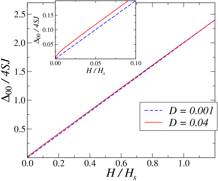
Figure 5: (Color online) $\Delta_{00}/4SJ$ v.s. $H/H_{s}$ for $D=0.001$ and $D=0.04$. Inset: same plot in the region of small fields.

$(\pi,\pi)$-gap.    The evolution of the ${\bf k}=(\pi,\pi)$ gap is much more interesting, because it corresponds to a mode which would be gapless in $D=0$ case. Using Eqs. (18) one arrives to:

$$\Delta_{\pi\pi}=4S\sqrt{2D\tan\varphi\left(1+D\tan\varphi-\frac{H}{8S}\sin\varphi\right)}\ ,$$ (25)

which clearly vanishes as $D\rightarrow 0$. The angle $\varphi$ is to be defined from Eq. (5) as before. Considering $D\ll 1$ limit one can identify three different regimes for the field: $H\sim D$, $H_{s}\gtrsim H\gg D$, and $H\simeq H_{s}$. After some algebra one can simplify Eq. (25) and obtain the following expressions for the gap in these regimes:

$$\Delta_{\pi\pi}\simeq\left\{\begin{array}[]{ll}\sqrt{4SD}\,\sqrt{H+4SD}&\ \ \mbox{for}\ \ H\sim D\ ,\\ \\ \sqrt{4SD}\,\sqrt{H\sqrt{1-\left(\displaystyle\frac{H}{8S}\right)^{2}}}&\ \ \mbox{for}\ \ H\gg D\ ,\\ \\ 4S\,\sqrt{3}\,D^{2/3}&\ \ \mbox{for}\ \ H=H_{s}\ .\end{array}\right.$$ (31)

These trends are clearly seen in our Fig. 6 for a small value of $D=0.001$. The gap evolves from $\Delta_{\pi\pi}/4S=D$ in zero field to its maximal value $\Delta_{\pi\pi}/4S=D^{1/2}$ at $H\simeq 0.707H_{s}$, and then has a minimum at $H_{s}$ where it reaches the value $\sqrt{3}D^{2/3}$ (marked by the dashed horizontal lines in Fig. 6). The origin of the maximum can be simply understood from Eq. (25) assuming $H\gg D$ and neglecting $D$ from everywhere except the common prefactor. This gives another expression for the $(\pi,\pi)$-gap in the intermediate-field regime:

$$\Delta_{\pi\pi}\simeq 4S\sqrt{D\sin 2\varphi},\ \ \mbox{with}\ \ \sin\varphi\approx\frac{H}{8S}\ .$$ (32)

This expression obviously has a maximum at $\varphi=\pi/4$ ($H=H_{s}/\sqrt{2}$), the canting angle at which the DM interaction is fully satisfied.

One can see that for the higher value of $D=0.04$ the maximum and minimum in the field-dependence of the gap are only weakly pronounced (inset of Fig. 6), while the zero-field gap $=D$ persists. Note that the zero-field gap is a salient feature of the model (1), intimately related to the phenomenon of the weak ferromagnetism. The origin of the minimum and of the unusual $2/3$ power of $D$ can be traced to the classical consideration we gave for the canting angle at the saturation field in Se. II.1.2. At $H=H_{s}$ we have $\cos\varphi\simeq D^{1/3}$, which yields $\Delta_{\pi\pi}\propto D^{2/3}$ from Eq. (25). For an interesting discussion of that fractional power see Ref. Mila, .

The minimum in $\Delta_{\pi\pi}(H)$ disappears, or, more precisely, merges with the maximum and becomes an inflection point, at a somewhat higher value of $D_{c}\simeq 0.066$. A similarly small number has been obtained in Ref. Mila, in the mean-field study of the Lieb-Mattis model.footnote6 It is surprising to have such a small “magic number” and one may wonder whether there is some hidden small parameter behind it. It turns out that it is a small difference of the powers of $D$ in $\Delta^{max}_{\pi\pi}$ and $\Delta^{min}_{\pi\pi}$ which is responsible for that smallness. One can estimate the “critical” value of $D$ at which the minimum disappears as the point where $\Delta^{max}_{\pi\pi}\approx\Delta^{min}_{\pi\pi}$. This gives: $D_{c}^{1/6}=1/\sqrt{3}$, or $D_{c}=1/27\simeq 0.037$. The actual number is about two times higher, but already at $D=0.04$ the minimum has almost faded away, see Fig. 6.

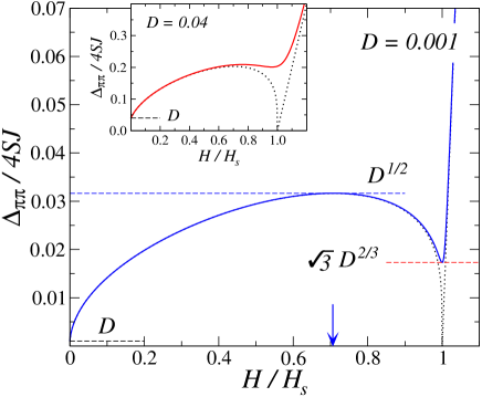
Figure 6: (Color online) Field dependence of $\Delta_{\pi\pi}/4SJ$ v.s. $H/H_{s}$ for $D=0.001$, Eq. (25). The gap values at $H=0$, $H=H_{s}/\sqrt{2}$, and $H=H_{s}$ are marked by the horizontal dashed lines. Dotted lines are: for $H<H_{s}$ – the low- and intermediate-field approximations for the gap, Eq. (31), for $H>H_{s}$ – the $D=0$ gap dependence $\Delta_{\pi\pi}=H-H_{s}$. Arrows mark $H=H_{s}/\sqrt{2}$. Inset: same for $D=0.04$.

To conclude the description of Fig. 6, the dotted line for $H<H_{s}$ is the convolution of the low- and intermediate-field results from Eq. (31), which gives a very close description for the gap behavior up to $H\sim H_{s}$. The dotted line for $H>H_{s}$ is the $D=0$ field dependence of the gap above the saturation field: $\Delta_{\pi\pi}=H-H_{s}$. One can see that the gap merges with this asymptote quickly. We add that the results similar to that in Fig. 6 were also reported for a 1D model with the DM interaction in Ref. YuLu, .

Our result for $\Delta_{00}$ and $\Delta_{\pi\pi}$ in the low-field regime, Eqs. (20) and (31), are in agreement with the results of the earlier works from the 1960s.Pinkus For the intermediate and high-field regimes our results in Eq. (31) agree with the results of the recent works on the coupled chainsSato and Lieb-Mattis model.Mila These works used the effective staggered field in place of the DM interaction that allows to simplify the model but introduces an approximation that neglects effects of order ${\cal O}(D)$ in the gaps. Such an approximation has created a discrepancy of these works with the earlier studies in the low-field regime. Namely, these recent works predict no weak ferromagnetism and no gap for the $(\pi,\pi)$-mode in zero field. Our results for $\Delta_{\pi\pi}$, Eqs. (25) and (5), provide a reconciliation of the earlier low-field and recent high-field studies. We also have provided a detailed analysis of the gap in the other spin-wave branch, the $(0,0)$-mode, Eqs. (19) and (20), which is gapless in zero field and has a $\propto\sqrt{H}$ behavior in a small field regime that can be mistaken with the results of Refs. Sato, ; Mila, for the $(\pi,\pi)$-mode.

This unified description of the behavior of the gaps in external field is also important as it clarifies the experimental prediction for the gaps’ dependence on the field. In the systems with the DM anisotropy which can be described by Eq. (1), instead of the literal $\propto\sqrt{DH}$ non-analytic behavior of the $(\pi,\pi)$-gap one should expect a non-analytic increase from a finite gap, $\propto\sqrt{D(H+4SD)}$, according to Eq. (31). As we will show in Sec. III, in real systems this behavior is further altered by the presence of other anisotropies.

II.3 Quantum corrections.

We gave an extensive discussion of the $(\pi,\pi)$-gap in Sec. II.2 because it will be also responsible for many of the changes in the behavior of quantum corrections due to the DM interaction.

As is mentioned in Introduction, very little systematic discussion of the influence of the DM interaction on the quantum effects in the Heisenberg-like systems has been given in the literature. The recent exception, Ref. Veillette, , considers the triangular-lattice AF$+$DM$+$field, to model the existing experiments in Cs₂CuCl₄. However, the results for that system are severely complicated by the other effects such as the field-dependence of the AF ordering vector and are hard to generalize to the other systems. Considering a much simpler, non-frustrated AF, we would like to ask a simple question: whether the quantum fluctuations are enhanced or suppressed by the DM interaction.

Formulae.   We are going to answer this question by analyzing the field-dependencies of the $1/S$-corrections to the ground-state energy, $\delta E$, local (on-site) magnetization, $\delta S$, and the uniform magnetization $\delta M$. As is discussed in Sec. II.2 the out-of-plane field case, ${\bf H}\|{\bf D}\|z$, is almost identical to the $D=0$ case, considered in Ref. Zhitomirsky, . Because of that, we are going to consider only the case of the in-plane field, ${\bf H}\perp{\bf D}\|z$.

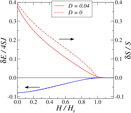
Figure 7: (Color online) $1/S$-corrections to the ground-state energy (left axis) and the on-site magnetization (right axis) for $D=0$ (dashed) and $D=0.04$ (solid) v.s. $H/H_{s}$, $S=1/2$.

The $1/S$-correction to the ground-state energy (per spin) is given in Eq. (12), which we rewrite here

$$\delta E=2S\sum_{\bf k}\Big{(}\nu_{\bf k}-C_{1}\Big{)}\ ,$$ (33)

using the dimensionless spin-wave energy $\nu_{\bf k}\equiv\omega_{\bf k}^{\perp}/4S$, Eq. (18), normalized to $4S$ to keep the $S$-proportionality explicit. The definition of the $1/S$-correction to the local (on-site) magnetization $\delta S$ follows straightforwardly from:

$$\langle S^{z_{0}}\rangle=S-\langle a^{\dagger}a\rangle=S-\delta S\ ,$$

$$\delta S=\langle a^{\dagger}a\rangle=\frac{1}{2}\sum_{\bf k}\left(\frac{C_{1}+C_{2}\gamma_{\bf k}}{\nu_{\bf k}}-1\right)\ ,$$ (34)

where the field- and DM-dependent constants $C_{i}$ are listed in Eq. (II.2.2). The classical part of the per-spin uniform magnetization is simply given by the canting angle: $M_{cl}=S\sin\varphi$, see Fig. 1(b). A more rigorous definition:

$$M=-\frac{dE}{dH}\ ,$$ (35)

where $E$ is the energy per spin from Eq. (4), leads to the same answer for the classical part and also yields the $1/S$-correction $\delta M$ as follows:

$$M=M_{cl}-\delta M=S\sin\varphi-\delta M\ ,$$

$$\delta M=2S\varphi^{\prime}\left[\sum_{\bf k}\frac{\partial\nu_{\bf k}}{\partial\varphi}-\frac{\partial C_{1}}{\partial\varphi}\right]\ ,$$ (36)

where

$$\varphi^{\prime}=\frac{\partial\varphi}{\partial H}=\frac{1}{8S}\ \frac{1}{\cos\varphi+D\sin\varphi\left(\displaystyle 1+\frac{1}{2\cos^{2}\varphi}\right)}\ ,$$

$$\mbox{and}\ \ \ \frac{\partial C_{1}}{\partial\varphi}=\frac{D}{\cos^{2}\varphi}\ ,$$ (37)

in which we used Eq. (5) and an explicit expression for $C_{1}=1+D\tan\varphi$ from Eq. (II.2.2). Note that the order of $\delta E$ is ${\cal O}(S)$ while $\delta S$ and $\delta M$ are ${\cal O}(1)$.

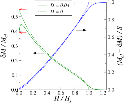
Figure 8: (Color online) Uniform magnetization (classical part + $1/S$-correction), right axis, and the $1/S$ part to the uniform magnetization normalized to its classical part, left axis, v.s. $H/H_{s}$. $D=0$ (dashed) and $D=0.04$ (solid). Arrows at the left axis show $\lim_{H\rightarrow 0}\lim_{D\rightarrow 0}$, Eq. (38), and $\lim_{D\rightarrow 0}\lim_{H\rightarrow 0}$, Eq. (39). $S=1/2$.

General features.    Having at hands expressions for the $1/S$ corrections to $E$, $\langle S^{z}\rangle$, and $M$, Eqs. (33), (II.3), and (II.3), together with the definitions of the spin-wave energy, Eq. (18), constants $C_{i}$, Eq. (II.2.2), and the canting angle, Eq. (5), one can calculate their field-dependence. Our Figure 7 shows the results for $\delta E/4S$ and $\delta S/S$ v.s. $H/H_{s}$, while Figure 8 shows the field dependence of $M/S=(M_{cl}-\delta M)/S$ and $\delta M/M_{cl}$, all for $S=\frac{1}{2}$ case. In both Figures the results for $D=0$ and $D=0.04$ are shown.

The overall field-dependence of the considered quantities is the same: quantum corrections are suppressed by the field.Zhitomirsky For the case of the pure Heisenberg model ($D=0$) the ground state above the saturation field ($H\geq H_{s}$) is classical and all quantum corrections vanish at $H=H_{s}$. Since in ${\bf H}\perp{\bf D}$ configuration the DM interaction prevents the full spin polarization by the field, quantum effects survive in the region $H>H_{s}$. However, with the further increase of the field they diminish quickly, see Figs. 7 and 8.

As is shown in Figures 7 and 8 different quantities are affected differently by the DM interaction. While we will elaborate on the detailed features of such effects below, we would like to note that the quantum corrections to all the considered quantities are undoubtedly suppressed by the DM interaction compared to the $D=0$ case for the fields $H\lesssim H_{s}$.

Besides the proliferation of the quantum fluctuations into the $H>H_{s}$ region and an overall suppression of them for $H<H_{s}$ there are two notable features shown in Figs. 7 and 8. First, while changes in the $1/S$-corrections to the energy due to a modest $D=0.04$ are hardly noticeable, changes in the quantum fluctuations of the on-site magnetization $\delta S$ are substantial. Moreover, the relative role of such DM-induced changes seems to be significantly amplified by the applied field. For instance, at $H=H_{s}/\sqrt{2}$ $\delta S$ is suppressed by almost 40% compared to its $D=0$ value due to the DM-term of the magnitude only 4% of $J$, see Fig. 7. Second, the behavior of $\delta M/M_{cl}$ v.s. $H$ is non-monotonic with significantly different zero-field limit of this quantity for the $D=0$ and $D\neq 0$ cases, see Fig. 8.

Uniform magnetization, $H=0$.    We would like to discuss the zero-field behavior of $\delta M/M_{cl}$ first. The reason for the choice of such a quantity is simple: the ratio of the quantum $1/S$ part, $\delta M$, to the classical magnetization, $M=S\sin\varphi$, shows explicitly the relative role of the quantum correction in the uniform magnetization. In addition, in the pure Heisenberg $D=0$ case all the terms in the $1/S$-expansion of the uniform magnetization vanish identically as $H\rightarrow 0$. Thus, at $D=0$ and $H\rightarrow 0$  $\delta M/M_{cl}$ is also related to the $1/S$-correction to the transverse susceptibility: $\chi=\chi_{cl}-\delta\chi=(M_{cl}-\delta M)/H$ [recall that $\sin\varphi=H/H_{s}$ when $D=0$]. Thus, using Eq. (II.3) and after some algebra the zero-field value of $\delta M/M_{cl}$ for $D=0$ case can be written as:

$$\lim_{H\rightarrow 0}\lim_{D\rightarrow 0}\frac{\delta M}{M_{cl}}=\frac{1}{2S}\sum_{\bf k}\gamma_{\bf k}\sqrt{\frac{1+\gamma_{\bf k}}{1-\gamma_{\bf k}}}=\frac{0.55115}{2S},$$ (38)

compare with the expression for $\delta\chi$ in Ref. Zhitomirsky, . This numerical value is marked by the upper arrow pointing towards the left $y$-axis in Fig. 8. One can see, however, that the DM interaction changes this quantity drastically. Neither the classical nor the quantum part of the uniform magnetization vanish in zero field anymore because of the weak ferromagnetism induced by the DM term. In other words, canting angle $\varphi$ does not go to zero at $H\rightarrow 0$, but approaches a finite value $\simeq D/2$. This leads to the following expression for the opposite order of limits:

$$\lim_{D\rightarrow 0}\lim_{H\rightarrow 0}\frac{\delta M}{M_{cl}}=\frac{1}{2S}\sum_{\bf k}\left(\frac{1}{\sqrt{1-\gamma^{2}_{\bf k}}}-1\right)=\frac{0.3932}{2S},$$ (39)

which is nothing but the expression for the $1/S$-correction to the on-site (staggered) magnetization $\delta S/S$ in the pure Heisenberg model at $H=0$. This value is marked by the lower arrow pointing towards the left $y$-axis in Fig. 8. Clearly, the behavior of $\delta M/M_{cl}$ v.s. $H$ and $D$ is singular as the limits $H\rightarrow 0$ and $D\rightarrow 0$ taken in different order lead to different results. For $D\neq 0$ there is a maximum in $\delta M/M_{cl}$ v.s. $H$ around $H\simeq D/2$ and then this quantity decreases roughly parallel to its $D=0$ counterpart, see Fig. 8.

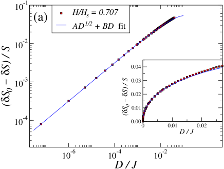
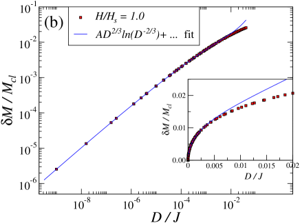
Figure 9: (Color online) The DM-induced changes in the $1/S$-corrections to (a) the on-site magnetization at $H=H_{s}/\sqrt{2}$ and (b) the uniform magnetization at $H=H_{s}$. Exact results obtained by using the numerical integration in (a) Eq. (II.3) and (b) Eq. (II.3) (squares) and the asymptotic expressions (a) Eq. (46) and (b) Eq. (52) (solid lines) are shown. (a) $A=1/2\pi S$, $B=0.48$, (b) $A=1/3\pi S$. $S=1/2$.

On-site magnetization.    To address the question on the sensitivity of the quantum component of the on-site magnetization, $\delta S$, to the DM interaction it is useful to analyze the quantity $\Delta S^{DM}=\delta S_{0}-\delta S$ as a function of $D$, where the subscript refers to the $D=0$ value. Using Eq. (II.3) one can write:

$$\frac{\Delta S^{DM}}{S}=\frac{\delta S_{0}-\delta S}{S}=\frac{1}{2S}\sum_{\bf k}\left(\frac{A_{\bf k}^{0}}{\nu_{\bf k}^{0}}-\frac{A_{\bf k}}{\nu_{\bf k}}\right)\ ,$$ (40)

where $A_{\bf k}=C_{1}+C_{2}\gamma_{\bf k}$ with $C_{1}$ and $C_{2}$ from Eq. (II.2.2) and $\nu_{\bf k}=\omega^{\perp}_{\bf k}/4S$ from Eq. (18) as before, and $\nu_{\bf k}^{0}$ and $A_{\bf k}^{0}$ are their $D=0$ limits, Eq. (13). One can show that in the limit $D\ll 1$ the difference $\delta S_{0}-\delta S$ is dominated by the contributions from the region in ${\bf k}$-space close to the $(\pi,\pi)$-point with the rest of the Brillouin zone contributing to the subleading terms only. It may thus be concluded that the behavior of the DM-induced change in $\delta S$ should be related to the DM-induced $(\pi,\pi)$-gap discussed in Sec. II.2.2. After some algebra one can obtain the asymptotic expressions:

$$\frac{\Delta S^{DM}}{S}\approx\frac{1}{2\pi S}\left\{\begin{array}[]{ll}D,&\ \ H=0\ ,\\ \\ \sqrt{D\sin 2\varphi},&\ \ D\ll H\lesssim H_{s}\ ,\\ \\ (\sqrt{3}-2)D^{2/3},&\ \ H=H_{s}\ ,\end{array}\right.$$ (46)

where $\sin\varphi\simeq H/H_{s}$. Thus, aside from a somewhat more subtle numerical coefficient for the result at $H=H_{s}$, the considered quantity follows almost identically the $D$-dependence of the $(\pi,\pi)$ gap, compare with Eqs. (31), (32). This asymptotic consideration also shows that except for the close vicinity of $H=0$ and $H=H_{s}$ the DM-induced change in $\delta S$ is proportional to $\propto D^{1/2}$. That is, it is significantly amplified compared to the other quantities and is not small already for the moderate values of $D$ as we observed in Fig. 7. To demonstrate the validity of this asymptotic result, Eq. (46), one can take the integral in Eq. (40) numerically and compare it with the results of Eq. (46) in the $D\ll 1$ limit. Such a comparison for a representative value of the field $H=H_{s}/\sqrt{2}$ ($\sin 2\varphi=1$ in Eq. (46)) is shown in Fig. 9(a) in both log-log and linear scales. The coefficient $B=0.48$ for the subleading term (${\cal O}(D)$) is used in this plot. One can see an excellent agreement of the numerical integration of an exact expression (squares) with the asymptotic formula, Eq. (46), (solid lines).

Uniform magnetization.    A similar analysis can be given to the other quantities. We have already discussed above the DM-induced changes in $\delta M/M_{cl}$ in the zero-field limit. Introducing $\Delta M^{DM}=\delta M_{0}-\delta M$ to characterize the effect of the DM interaction on the quantum component of the uniform magnetization, where $\delta M_{0}$ is the $D=0$ limit of $\delta M$, after some algebra one obtains the asymptotic expressions:

$$\frac{\Delta M^{DM}}{M_{cl}}\approx\frac{1}{2S}\left\{\begin{array}[]{ll}0.1574,&\ H=0\ ,\\ \\ A_{1}D,&\ D\ll H\lesssim H_{s}\ ,\\ \\ \displaystyle\frac{2D^{2/3}}{3\pi}\ln D^{2/3},&\ H=H_{s}\ .\end{array}\right.$$ (52)

Clearly, these are less trivial dependencies than for the on-site magnetization, Eq. (46). The number for the $H=0$ case is simply the difference of the results in Eqs. (38) and (39) discussed before. For the intermediate-field regime $D\ll H\lesssim H_{s}$ the DM-induced changes in the uniform magnetization are not dominated by any particular region in the ${\bf k}$-space, but are accumulated over the entire BZ. Therefore, there is no straightforward relation between the $D$- or $H$-dependence of the $(\pi,\pi)$-gap and $\Delta M^{DM}$. The expression for $A_{1}(H)$ is rather cumbersome and we only list its value for a representative field: $A_{1}(H_{s}/\sqrt{2})=0.1580$. On the contrary, in the regime $H=H_{s}$ the DM-induced changes in $\delta M/M_{cl}$ are dominated by the vicinity of the $(\pi,\pi)$-gap, but only with the logarithmic accuracy, see Eq. (52), since the subleading term is ${\cal O}(D^{2/3})$. To demonstrate the validity of the latter asymptotic expression we evaluated $(\delta M_{0}-\delta M)/M_{cl}$ numerically using Eq. (II.3) and compared it with the results in Eq. (52) for $H=H_{s}$. An excellent agreement between the numerical (squares) and asymptotic expressions (solid lines) is shown in Fig. 9(b).

Energy.    A similar consideration can be given to the $1/S$-correction to the energy. For the intermediate-field regime $D\ll H\lesssim H_{s}$ one finds that $(\delta E_{0}-\delta E)/4S=A_{3}D+{\cal O}(D^{3/2})$, same as $\delta M^{DM}$ but with much smaller numerical coefficient. For example, for $H=H_{s}/\sqrt{2}$ the expression for the coefficient $A_{3}$ can be simplified to

$$A_{3}=\frac{1}{2}\sum_{\bf k}\left(\frac{1-\gamma_{\bf k}^{2}/2}{\sqrt{1+\gamma_{\bf k}}}-1\right)=0.0259.$$ (53)

At the saturation field the energy correction can be approximately written as:

$$\frac{\delta E}{4S}=\frac{D^{4/3}}{4\pi}\ln\left(\frac{D^{2/3}}{\lambda}\right)+{\cal O}(D^{2}),$$ (54)

which contains an extra power of $D^{2/3}$ in comparison with $\delta M/M_{cl}$, Eq. (52).

Summary.   Altogether, the quantum $1/S$ corrections are changed substantially under the influence of the DM interaction. Many of the considered changes depend on $D$ non-analytically, see Eqs. (46), (52), and (54), and some exhibit a singular behavior as for the case of $\delta M/M_{cl}$ in $(H,D)\rightarrow 0$ limit, see Eqs. (38), (39), and Fig. 8. The most substantial change is seen in the on-site magnetization where for the broad field range $\delta S_{0}-\delta S\propto D^{1/2}$, see Eq. (46) and Fig. 7. Except for the vicinity of the saturation field where the quantum effects are enhanced (or, rather, induced for $H>H_{s}$), the quantum fluctuations are suppressed by the DM interaction, see Figs. 7 and 8.

III K₂V₃O₈

III.1 Experiments and Hamiltonian

K₂V₃O₈ has been studied experimentally by magnetometry and neutron scattering, as reported in Ref. Lumsden, . This material contains weakly coupled square lattice planes of spins $S=\frac{1}{2}$. The spins interact antiferromagnetically with the superexchange constant $J=12.6$K. In the ground state spins are pointing along the $z$-axis while in a low external field ($H<1$T) two types of transitions were seen. For the field along the $z$-axis the well-known “spin-flop”-type transition occurs at $H_{SF}$: spins suddenly “flop” in the $x-y$ plane and cant towards the field upon further increase of the field in a configuration similar to Fig. 1(a). For the field ${\bf H}\perp z$ an unusual “spin-rotation” transition is seen: spins perform a rotation by $\pi/2$ angle gradually from along the $z$-axis into the $x-y$ plane within a very small field range $0<H<H_{SR}$. Above the “spin-rotation” field $H_{SR}$ spins are in the $x-y$ plane and cant towards the field in a configuration similar to Fig. 1(b). Such a behavior made the authors of Ref. Lumsden, to conclude that there are small anisotropies of two types which accompany the superexchange in this material: the easy-axis anisotropy along the $z$-axis and the DM-anisotropy also directed along the $z$-axis. Therefore, K₂V₃O₈ is described by our Hamiltonian (1) with an additional easy-axis term:

$$\delta{\cal H}_{ea}=E\sum_{\langle ij\rangle}S^{z}_{i}S^{z}_{j}\ .$$ (55)

As is shown in Ref. Lumsden, , with an appropriate choice of parameters the Hamiltonian (1)$+$(55) describes excellently all the observed transitions.

As is mentioned in Sec. II, although the easy-axis constant $E$ is of the order of ${\cal O}(D^{2})$, it competes with the DM-term on equal footing. While for an ideal staggered configuration of the DM vectors it is expected that the easy-axis constant is $E=D^{2}/2$ and the system possesses a hidden $O(3)$ symmetry,Shekhtman1 a non-staggered component of the DM vector generally breaks such a high symmetry and leads to $E<D^{2}/2$.Yildrim In realistic systems, like K₂V₃O₈ the easy-axis term is, de facto, $E>D^{2}/2$ due to some other microscopic processes. We thus consider $D$ and $E$ as independent parameters, but still $E\sim D^{2}$. In the rest of the Section we consider the experimentally relevant case $E>D^{2}/2$ and discuss the case $E<D^{2}/2$ in the end.

One can show that for the case of vector ${\bf D}$ being along the “easy” axis and for $E>D^{2}/2$ (we continue to use $J=1$ units here), the easy-axis anisotropy overcomes the DM-term in the ground state. That is, instead of staying in the plane $\perp{\bf D}$ and canting towards each other, as favored by the DM interaction, spins align along the “easy” axis as dictated by the easy-axis term and as if the DM-term was absent. Therefore, in the ground state of this Hamiltonian at $H=0$ and $E>D^{2}/2$ there is no weak ferromagnetism and the DM interaction is “hidden”. However, the external field helps to reveal the presence of the DM interaction in the system. It is the interplay of the easy-axis and the DM-term which causes an unusual spin rotation from the $z$-axis into the $x-y$ plane in K₂V₃O₈.

III.2 Ground state and excitation spectrum in a field

We thus consider the Hamiltonian (1)$+$(55) as a starting point and take the experimental estimate for the DM constant $D=0.04$, Ref. Lumsden, . For the easy-axis constant we use the value $E=0.0017$, somewhat higher than estimated in Ref. Lumsden, , for the reasons discussed below.

Before the technical discussion we would like to describe the field evolution of the ground state from the symmetry point of view. In zero field for $H<H_{SF}(H_{SR})$ the continuous $O(3)$ symmetry is broken by the easy-axis term to a discrete Ising-like one. Thus, all the excitations in such a phase should be gapped. For ${\bf H}\|z$ above the spin-flop field, $H>H_{SF}$, the continuous symmetry is restored to $O(2)$. This symmetry corresponds to the freedom of choice of the direction of the spins’ component in the $x-y$ plane. Since the DM vector is also $\|z$, its presence does not change this consideration except that the spins acquire a small canting angle towards each other in the $x-y$ plane, see Fig. 1(a). Therefore, one of the magnon branches should be gapless in this phase. This is identical to the ${\bf H}\|{\bf D}$ field configuration discussed in Secs. II.1.1, II.2.1 without the easy-axis anisotropy. For the in-plane field ${\bf H}\perp{\bf D}\|z$ above the spin-rotation field, $H>H_{SR}$, all the continuous symmetries remain broken and the ground state is identical to the one considered in Sec. II.1.2 and Fig. 1(b) where spins are in the $x-y$ plane and are canted towards the field. In such a phase no gapless excitation should exist.

With these ideas in mind we will analyze classical spin configurations and excitation spectrum of the Hamiltonian (1)$+$(55). Because of the easy-axis term there are two different phases for each of the field directions: below and above the spin-flop (spin-rotation) transition for ${\bf H}\|z$ (${\bf H}\perp z$).

III.2.1 Out-of-plane field.

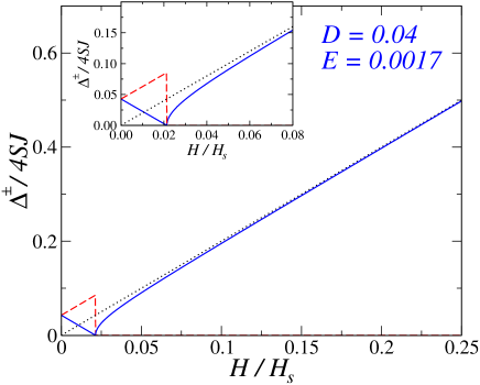
Figure 10: (Color online) The field-evolution of the gaps for the spin-flop field configuration ${\bf H}\|{\bf D}\|z$. The spin-flop transition occurs at $H_{SF}$, Eq. (60). Below the transition the gaps depend linearly on $H$, Eq. (62). Above the transition one of the gaps is zero (dashed) and the other corresponds to a uniform precession of the field-induced magnetization (solid), Eq. (64). The uniform precession mode for the $E=D=0$ case is shown by the dotted line ($\Delta=H$). Inset: same results in the region of the small fields. Saturation field for K₂V₃O₈ is $H_{s}=8SJ=37.6$T.

For the ${\bf H}\|{\bf D}\|z$ configuration the classical energy of the Hamiltonian (1)$+$(55) can be written as:

$$\frac{E_{cl}}{2NS^{2}}=\cos\theta_{A}\cos\theta_{B}(1+E)$$

$$\phantom{\frac{E_{cl}}{2NS^{2}}=}-\sin\theta_{A}\sin\theta_{B}\left(\cos 2\varphi+D\sin 2\varphi\right)$$ (56)

$$\phantom{\frac{E_{cl}}{2NS^{2}}=}-\frac{H}{4S}\left(\cos\theta_{A}+\cos\theta_{B}\right)\ ,$$

where $\theta_{A}$ and $\theta_{B}$ are the angles with the $z$-axis made by spins in the $A$ and $B$ sublattice, respectively. $\varphi$ is the angle in the $x-y$ plane as in Fig. 1(a). Using the symmetry arguments one can show that for the case $E>D^{2}/2$ two choices of the spin configuration are possible: (i) $\theta_{A}=0$, $\theta_{B}=\pi$, and (ii) $\theta_{A}=\theta_{B}=\theta$, as in Fig. 1(a). Needless to say, these two choices correspond to $H<H_{SF}$ and $H>H_{SF}$, respectively. For the first choice the spins are pointing along the $z$-axis and the classical energy is field- and DM-independent:

$$\frac{E_{cl}^{(1)}}{2NS^{2}}=-(1+E)\ .$$ (57)

For the second choice the energy is minimized by the following choice of angles:

$$\varphi=\frac{1}{2}\tan^{-1}D\ ;\ \ \ \cos\theta=\frac{H}{8S}\ \frac{2}{1+E+\sqrt{1+D^{2}}}\ ,$$ (58)

where $\varphi$ gives a small field-independent canting of spins in the $x-y$ plane. For small fields spins are almost in the $x-y$ plane as $\theta\approx\pi/2$, all in a very close similarity with our discussion of the DM-only case, Sec. II.1.1, Fig. 1(a), and Eq. (3). Using these angles (58) one can rewrite the classical energy as:

$$\frac{E_{cl}^{(2)}}{2NS^{2}}=-\sqrt{1+D^{2}}-\frac{H^{2}}{16S^{2}(1+E+\sqrt{1+D^{2}})}\ .$$ (59)

From the condition $E_{cl}^{(1)}=E_{cl}^{(2)}$ we can now find the field at which the spin-flop transition between the two spin configurations occurs. This gives:

$$H_{SF}=4S\sqrt{2E-D^{2}+E^{2}}\simeq 4S\sqrt{2E-D^{2}}\ ,$$ (60)

which is well-defined only if $E>D^{2}/2$. Because $E\sim D^{2}\ll 1$ one can neglect $E^{2}$, $D^{4}$, etc. as being extremely small. One can verify that the first derivative of the energy with respect to field has a jump as is expected for the first-order transition. The angles also experience discontinuous jumps to finite values at $H_{SF}$ as can be inferred from Eq. (58).

The field evolution of the excitation spectrum within the spin-flop problem has been studied in the past and is well-known (see, e.g., Ref. Tennant, ). In our case there are some quantitative changes due to the DM-term, but the overall behavior is very similar. Below the transition there are two branches:

$$\omega_{\bf k}^{\pm}=4S\sqrt{(1+E)^{2}-\gamma_{\bf k}^{2}(1+D^{2})}\pm H\ ,$$ (61)

with the gaps:

$$\Delta^{\pm}=H_{SF}\pm H\ ,$$ (62)

where the spin-flop field is given in Eq. (60).

Above the spin-flop transition the spectrum can be written as:

$$\omega_{\bf k}=4S\sqrt{1+D^{2}}\sqrt{(1+\gamma_{\bf k})(1-\delta_{1}\gamma_{\bf k})}\ ,$$ (63)

$$\mbox{where}\ \delta_{1}=\left(1+E-\frac{4(H/H_{s})^{2}}{1+E+\sqrt{1+D^{2}}}\right)\frac{1}{\sqrt{1+D^{2}}}\ ,$$

with one mode gapless, $\Delta_{\pi\pi}\equiv 0$, and the other mode having a gap which can be written as:

$$\Delta_{00}=\sqrt{\frac{2\sqrt{1+D^{2}}}{1+E+\sqrt{1+D^{2}}}}\ \sqrt{H^{2}-H_{SF}^{2}}\ .$$ (64)

This mode reaches the uniform precession behavior $\Delta\simeq H$ at $H\gg H_{SF}$. All these field-dependencies of the gaps are shown in our Fig. 10. One can see a jump in one of the gaps associated with the spin-flop transition. The dotted line is $\Delta=H$ ($E=D=0$ result). As we discussed above, one of the modes is necessarily gapless for $H>H_{SF}$, same as for the $E=0$ case, Sec. II.2.1.

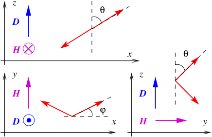
Figure 11: (Color online) The projections of the spin arrangement on the $x-z$-, $x-y$-, and $y-z$-planes within the spin-rotation phase $0<H<H_{SR}$. While $\varphi$ is the angle between the projections of spins on the $x-y$ plane and the $x$-axis, $\theta$ is the angle between the actual spin direction and the $z$-axis. ${\bf H}$ is chosen along the $y$-axis.

III.2.2 In-plane field.

For the ${\bf H}\perp{\bf D}\|z$ field configuration the spin arrangement within the spin-rotation phase $0<H<H_{SR}$ is given in Fig. 11. Note that $\varphi$ is the angle between the projections of spins on the $x-y$ plane and the $x$-axis, while $\theta$ is the angle between the actual spin direction and the $z$-axis. One can see that the angle with the $z$-axis $\theta_{B}=\pi-\theta_{A}$ for the spins in different sublattices. Both angles, $\varphi$ and $\theta$, are coupled non-trivially in the classical energy of the Hamiltonian (1)$+$(55) which can be written as:

$$\frac{E_{cl}}{2NS^{2}}=-\cos^{2}\theta(1+E)$$ (65)

$$\phantom{\frac{E_{cl}}{2NS^{2}}=}-\sin^{2}\theta\left(\cos 2\varphi+D\sin 2\varphi\right)-\frac{H}{2S}\sin\theta\sin\varphi\ .$$

Minimizing the energy, after some algebra, leads to the following expressions for the angles:

$$\tan\varphi=\frac{E}{D}\ ;\ \ \ \sin\theta=\frac{H}{4S}\ \frac{\sqrt{D^{2}+E^{2}}}{2E-D^{2}+E^{2}}\ ,$$ (66)

Somewhat surprisingly, the $\varphi$ angle remains field-independent throughout the spin-rotation phase. Since the easy-axis interaction $E$ is of the same order as $D^{2}\ll 1$, $\varphi\approx E/D$ is also small. On the contrary, $\theta$ changes drastically (but continuously) from $0$ at $H=0$ to $\pi/2$ at the critical field $H_{SR}$. The latter can be found from Eq. (66) as:

$$H_{SR}=4S\ \frac{2E-D^{2}}{D}\ ,$$ (67)

where we omitted ${\cal O}(E^{2})$ terms.

For the fields above the transition, $H>H_{SR}$, a different solution minimizes the classical energy in Eq. (65): $\theta=\pi/2$ is constant and $\varphi$ is field-dependent. That is, the spins are lying in the $x-y$ plane as depicted in Fig. 1(b). It is easy to see that for $\theta=\pi/2$ Eq. (65) reduces to the classical energy for the DM-only case, Eq. (4). Thus, the easy-axis term is effectively “switched-off” by the field for $H>H_{SR}$. Because of that the field-dependence of the canting angle $\varphi$ also remains the same as in Sec. II.1.2, Eq. (5).

Using the canting angles, Eqs. (66) and (5), one can simplify the expressions for the classical energies below and above the spin-rotation transition to:

$$\frac{E^{<}_{cl}}{2NS^{2}}=-(1+E)-\frac{H^{2}}{16S^{2}}\ \frac{E}{2E-D^{2}}\ ,$$ (68)

$$\frac{E^{>}_{cl}}{2NS^{2}}=-1-\frac{1}{2}\left(\frac{H}{4S}+D\right)^{2}\ ,$$ (69)

where ${\cal O}(E^{2})$ terms are neglected. From these formulae one can verify that the spin-rotation transition is of the second order as the energy and its first derivative are continuous through the transition. The angles also change continuously at $H_{SR}$ as can be seen, for instance, for $E,D^{2}\ll 1$: $\varphi^{<}=E/D$ matches with $\varphi^{>}=D/2+H/8S$ at $H=H_{SR}$, Eq. (67).

These canting angles can be translated directly into the field-induced uniform magnetization which has been measured as a function of applied field, see Ref. Lumsden, . In small field the uniform magnetization depends linearly on field, but has different slopes for $H<H_{SR}$ and $H>H_{SR}$. On the other hand, such slopes can be extracted from our Eqs. (68) and (69) which give:

$$\left(\frac{dM^{>}}{dH}\right)\bigg{/}\left(\frac{dM^{<}}{dH}\right)=1-\frac{D^{2}}{2E}\ .$$ (70)

This relation is useful to extract the ratio $D^{2}/E$ because the slope in the magnetization v.s. field can be measured rather reliably and is the subject of less experimental error than, say, the transition field itself. It is using this relation and $D=0.04$ we have extracted the value $E=0.0017$ for K₂V₃O₈ used throughout this Section.

After the easy-axis and the DM constants are chosen one can find the $T=0$ values of the spin-flop and spin-rotation fields from Eqs. (60) and (67). Using the values of $g_{c}=1.922$ and $g_{ab}=1.972$ for K₂V₃O₈ reported in Ref. Lumsden, one finds: $H_{SF}\approx 0.85$T and $H_{SR}\approx 0.89$T. These theoretical values are within the same range as $H_{SF}^{exp}=0.85$T and $H_{SR}^{exp}=0.65$T found in Ref. Lumsden, from the neutron scattering and magnetization measurements and $H_{SF}^{exp}=0.95$T and $H_{SR}^{exp}=0.55$T estimated from the upturn in the thermal conductivity v.s. field in Ref. Sales, . Since all these experimental results were obtained at a finite temperature of the order of the Néel ordering temperature for this material, the differences between the theoretical results and the data are to be expected. The closer agreement with the data for the spin-flop field are due to the first-order nature of that transition. It is knownTennant that the critical field for the spin-flop transition is only weakly temperature-dependent. For the spin-rotation transition, on the other hand, one can expect a suppression of the critical field with the temperature. Overall, the theoretical results for the critical fields are in a close accord with the experimental data.

One can now address the field-dependence of the excitation spectrum for the spin-rotation problem. As is explained in Sec. II.2, we need the field-dependence of the canting angles, a transformation from the local to the laboratory frame for spins, and the subsequent quantization of the spin Hamiltonian to obtain the spectrum. While above the transition, $H>H_{SR}$, the first two steps are essentially identical to the ones performed for the DM-only case in Sec. II.2.2, below the transition, $H<H_{SR}$, this procedure requires an additional and a somewhat cumbersome algebra. We thus simply provide here the results for the gaps in the spin-rotation phase $H<H_{SR}$:

$$\Delta_{00}=\sqrt{4SDH_{SR}\left(1+\frac{HH_{SR}}{4SD}\right)}\ ,$$ (71)

$$\Delta_{\pi\pi}=\sqrt{4SDH_{SR}\left(1-\frac{H^{2}}{H_{SR}^{2}}\right)}\ ,$$ (72)

where $H_{SR}$ is from Eq. (67) and we neglect ${\cal O}(E^{2})$ terms as before.

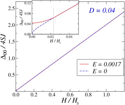
Figure 12: (Color online) $\Delta_{00}/4SJ$ v.s. $H/H_{s}$ for the in-plane field direction, $D=0.004$, and two values of $E$: $E=0.0017$ (solid), Eqs. (71) and (74), and $E=0$ (dashed), Eq. (19). Inset: same plot in the region of small fields. The spin-rotation transition is marked by the dotted vertical line. Saturation field for K₂V₃O₈ is $H_{s}=8SJ=37.6$T.

For the fields above the transition, $H>H_{SR}$, the changes with respect to the DM-only case, Sec. II.2.2, are rather incremental and we can afford listing the parameters of the spin-wave Hamiltonian:

$$C_{1}=1+D\tan\varphi\ ,$$

$$C_{2}+C_{3}=-\cos 2\varphi-D\sin 2\varphi\ ,$$ (73)

$$C_{2}-C_{3}=1+B\ ,$$

which one can compare to an equivalent expression in Eq. (II.2.2). Thus, the easy-axis term leads to rather obvious changes in the spin-wave energy, Eq. (18). The gaps are changed accordingly and are given by:

$$\Delta_{00}=4S\sqrt{\frac{H}{2S}\sin\varphi\left(1+\frac{1}{2}D\tan\varphi+E\right)}\ ,$$ (74)

$$\Delta_{\pi\pi}=4S\sqrt{2(D\tan\varphi-E)}$$ (75)

$$\phantom{\Delta_{\pi\pi}=4S}\times\sqrt{\left(1+D\tan\varphi-\frac{H}{8S}\sin\varphi\right)}\ ,$$

which should be compared to the DM-only results, Eqs. (19) and (25), respectively. It is important to note that in the vicinity of the transition field the $(\pi,\pi)$-gap has the following non-analytic field-dependence:

$$\Delta_{\pi\pi}=\sqrt{4SD(H-H_{SR})}\ ,$$ (76)

for $H>H_{SR}$. This is reminiscent of Eq. (31) for the $H\ll H_{s}$ case, but with the field “shifted down” by $H_{SR}+4SD$.

Our results for the field-dependence of the $\Delta_{00}$ and $\Delta_{\pi\pi}$ gaps, both below and above the spin-rotation transition, together with the results for the DM-only ($E=0$) case are shown in Figures 12 and 13, respectively. One can see that for the $\Delta_{00}$ gap above the transition the results for K₂V₃O₈ are essentially indistinguishable from the DM-only case. It can be shown that the difference between them scales as $\propto{\cal O}(EH)={\cal O}(D^{2}H)$. The changes in $\Delta_{\pi\pi}$ with respect to the DM-only case are more substantial. They scale as ${\cal O}(E/D)$ for the fields $H\gtrsim H_{SR}$ but diminish closer to the saturation field. Thus, the major effect of the easy-axis anisotropy on the excitation spectrum is the effective “off-set” of the external field by $H_{SR}+4SD$, as can be seen from comparison of Eqs. (76) and (31).

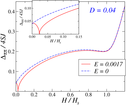
Figure 13: (Color online) $\Delta_{\pi\pi}/4SJ$ v.s. $H/H_{s}$ for the in-plane field direction, $D=0.004$, and two values of $E$: $E=0.0017$ (solid), Eqs. (72) and (75), and $E=0$ (dashed), Eq. (25). Inset: same plot in the region of small fields. Saturation field for K₂V₃O₈ is $H_{s}=8SJ=37.6$T.

III.2.3 $E\leq D^{2}/2$ case.

For completeness, we briefly discuss here the case $E<D^{2}/2$. In such a case the ground state and the spectrum field-dependencies are qualitatively the same as in the DM-only case (1) considered in Secs. II.1 and II.2. In fact, for the most interesting ${\bf H}\perp{\bf D}$ configuration the canting angle in the ground state is simply identical to Eq. (5) because the easy-axis anisotropy is effectively switched-off. In particular, the zero-field ground state for $E<D^{2}/2$ possesses the same uniform magnetization as if the easy-axis term would be absent. Interestingly enough, the high- and intermediate-field behavior of the $(\pi,\pi)$-gap also depends only on the DM-term, $\Delta_{\pi\pi}\propto(DH)^{1/2}$ for $H\gg D$. On the other hand, the zero-field gap in this case is reduced: $\Delta_{\pi\pi}=4S\sqrt{D^{2}-2E}$. Thus, the zero-field canting angle $\varphi\simeq D/2$ is not in one-to-one correspondence anymore with the zero-field $(\pi,\pi)$-gap, in contrast to the DM-only case, model (1).

A particular case $E=D^{2}/2$ is also interesting as it shows no gap in zero-field, yet a finite-field behavior of the gap is governed by the DM-term: $\Delta_{\pi\pi}\propto(DH)^{1/2}$, the result obtained in Refs. Sato, ; Mila, . Another interesting feature of that case is that the classical energy in zero-field, Eq. (65), is degenerate for any choice of $\theta$, while $\varphi=\frac{1}{2}\tan^{-1}D\simeq D/2$. That is, the weak ferromagnetism with the uniform magnetization of an arbitrary strength from the range $0<M\lesssim SD/2$ can occur in zero-field ground state as a result of the spontaneous choice of $\theta$ in the spin configuration depicted in Fig. 11. This scenario has been also discussed on Ref. Shekhtman1, .

III.2.4 Summary.

Altogether, an additional easy-axis anisotropy introduces some new transitions in the physics of a realistic system in comparison with the DM-only case, but leaves most of the results for the field above the corresponding transition unchanged. That is, for the out-of-plane field configuration one of the gaps in the spin-wave spectrum behaves similarly to a uniform precession mode, $\Delta\approx H$, while the other mode stays gapless. For the in-plane field both modes are gapped. One of them is the uniform precession mode while the other depends non-analytically on the field and shows a non-trivial behavior in high field. We would like to note that some indications of such a drastically different behavior of the gaps for different field directions have been observed in the field-dependence of the thermal conductivityfuture in K₂V₃O₈, see Ref. Sales, . One of the crucial differences of the K₂V₃O₈ spectrum field-dependence from the idealized DM-only case, Eq. (1), is the effective off-set of the field for the in-plane field direction, leading to the $\propto\sqrt{D(H-H_{SR})}$ behavior of the gap. Thus, in a realistic system, the low-field behavior of the DM-induced gap is more delicate than simple $\propto\sqrt{DH}$ suggested recently.Affleck ; Sato ; Mila

IV Conclusions

We conclude by summarizing our results. We have studied the effects of external field on the properties of an ordered Heisenberg antiferromagnet with the DM interaction. Utilizing the spin-wave theory we have calculated the quantum correction to the energy, on-site magnetization, and uniform magnetization v.s. $H$ and $D$. We have shown that the spin-wave excitations exhibit an unusual field-evolution of the gaps which leads to various non-analytic dependencies of the quantum corrections. We have found that the gap in one of the magnon branches follows a particularly interesting behavior v.s. field for a specific field direction: $\Delta_{\pi\pi}$ is $\propto D$, $\propto D^{1/2}$, or $\propto D^{2/3}$ depending on the field. A similar behavior is reflected in some of the quantum corrections as well. We have demonstrated that for the fields $0<H\lesssim H_{s}$ the DM interaction suppresses quantum fluctuations. The on-site ordered moment is affected most strongly by such a suppression. It is only in the regime of the field close to the saturation where the DM term enhances quantum fluctuations, effectively leading to a proliferation of the quantum effects into the classical saturated phase. We have shown that some quantum corrections are singular in the limit of $H,D\rightarrow 0$.

We also have considered K₂V₃O₈ which is well described by the spin-$\frac{1}{2}$, Heisenberg AF on the two-dimensional square lattice, with the additional DM and easy-axis anisotropies. We have demonstrated that K₂V₃O₈ is an excellent candidate for the observation of the unusual field-dependence of the gaps, characteristic to the 2D and 3D AFs. In fact, an additional easy-plane anisotropy makes it potentially possible to observe a non-analytic $\Delta\propto\sqrt{D(H-H_{SR})}$ behavior of the gap.

- (1) A. Zheludev, Z. Honda, Y. Chen, C. L. Broholm, K. Katsumata, and S. M. Shapiro, Phys. Rev. Lett. 88, 077206 (2002).
- (2) G. Chaboussant, M.-H. Julien, Y. Fagot-Revurat, M. Hanson, L.P. Lévy, C. Berthier, M. Horvatić, and O. Piovesana, Eur. Phys. J. B 6, 167 (1998).
- (3) T. Nikuni, M. Oshikawa, A. Oosawa, and H. Tanaka, Phys. Rev. Lett. 84, 5868 (2000); M. Jaime, V. F. Correa, N. Harrison, C. D. Batista, N. Kawashima, Y. Kazuma, G. A. Jorge, R. Stern, I. Heinmaa, S. A. Zvyagin, Y. Sasago, and K. Uchinokura, Phys. Rev. Lett. 93, 087203 (2004); V. S. Zapf, D. Zocco, M. Jaime, N. Harrison, A. Lacerda, C. D. Batista, and A. Paduan-Filho, cond-mat/0505562.
- (4) H. Kageyama, K. Yoshimura, R. Stern, N. Mushnikov, K. Onizuda, M. Kato, K. Kosuge, C.-P. Slichter, T. Goto, and Y. Ueda, Phys. Rev. Lett. 82, 3168 (1999); T. Ono, H. Tanaka, O. Kolomiyets, H. Mitamura, T. Goto, K. Nakajima, A. Oosawa, Y. Koike, K. Kakurai, J. Klenke, P. Smeibidle, and M. Meissner, J. Phys.: Condens. Matter 16, S773 (2004).
- (5) O. Cépas, K. Kakurai, L.P. Regnault, T. Ziman, J.P. Boucher, N. Aso, M. Nishi, H. Kageyama, and Y. Ueda, Phys. Rev. Lett. 87, 167205 (2001).
- (6) D. C. Dender, P. R. Hammar, D. H. Reich, C. Broholm, and G. Aeppli, Phys. Rev. Lett. 79, 1750 (1997).
- (7) J. Sirker, A. Weiße, O. P. Sushkov, Europhys. Lett. 68, 275 (2004); cond-mat/0409530.
- (8) T. Sakai and H. Shiba, J. Phys. Soc. Jpn. 63, 867 (1994) and references therein.
- (9) M. Oshikawa and I. Affleck, Phys. Rev. Lett. 79, 2883 (1997); Phys. Rev. B 60, 1038 (1999).
- (10) J. Z. Zhao, X. Q. Wang, T. Xiang, Z. B. Su, L. Yu, Phys. Rev. Lett. 90, 207204 (2003).
- (11) M. Sato and M. Oshikava, Phys. Rev. B 69, 054406 (2004).
- (12) J.-B. Fouet, O. Tchernyshyov, and F. Mila, Phys. Rev. B, 70 174427 (2004).
- (13) P. Pinkus, Phys. Rev. Lett. 5, 13 (1960).
- (14) The DM corrections also attracted attention in the context of the high-Tc materials, in particular La2CuO4, where the DM term plays an important role in orienting spins in the CuO2 plane, see Ref. Trugman, .
- (15) D. Coffey, K. S. Bedell, and S. A. Trugman, Phys. Rev. B 42, 6509 (1990).
- (16) I. E. Dzyaloshinskii, J. Phys. Chem. Solids 4, 241 (1958); T. Moriya, Phys. Rev. Lett. 4, 228 (1960).
- (17) R. Coldea, D. A. Tennant, K. Habicht, P. Smeibidl, C. Wolters, and Z. Tylczynski, Phys. Rev. Lett. 88, 137203 (2002).
- (18) M. Y. Veillette, J. T. Chalker, and R. Coldea, cond-mat/0501347.
- (19) The case of Cs2CuCl4 is severely complicated by the field-dependence of the AF ordering vector.
- (20) V. N. Kotov, M. E. Zhitomirsky, M. Elhajal, and F. Mila, Phys. Rev. B 70, 214401 (2004).
- (21) M. Elhajal, B. Canals, R. Sunyer i Borrell, and C. Lacroix, cond-mat/0503009.
- (22) M. D. Lumsden, B. C. Sales, D. Mandrus, S. E. Nagler, and J. R. Thompson, Phys. Rev. Lett. 86, 159 (2001).
- (23) Earlier studies of the copper formate tetrahydrate (CFT), a quasi-2D spin- AF on a square lattice, by electron spin resonance have indicated a spin reorientation transition in modest fields similar to the one in K2V3O8: M. S. Seehra and T. G. Castner, Jr., Phys. Rev. B 1, 2289 (1970). In that work the field-dependence of the gaps has been analyzed with results somewhat similar to the ones we predict for K2V3O8.
- (24) Note, that we also consider the most common case of the staggered DM interaction. The uniform DM interaction (without ) would lead to a spiral-like ordering, see e.g. T. Nikuni and A. E. Jacobs, Phys. Rev. B 57, 5205 (1998).
- (25) L. Shekhtman, O. Entin-Wohlman, and A. Aharony, Phys. Rev. Lett. 69, 836 (1992).
- (26) L. Shekhtman, A. Aharony, and O. Entin-Wohlman, Phys. Rev. B 47, 174 (1992).
- (27) T. Yildirim, A. B. Harris, A. Aharony, and O. Entin-Wohlman, Phys. Rev. B 52, 10239 (1995).
- (28) M. E. Zhitomirsky and T. Nikuni, Phys. Rev. B 57, 5013 (1998).
- (29) M. E. Zhitomirsky and A. L. Chernyshev, Phys. Rev. Lett. 82, 4536 (1999).
- (30) A consideration of such an instability in the presence of anisotropies will be given in a future work.
- (31) The coefficient in the transverse field in Ref. Mila, should be equal to in the original DM interaction. Thus, the “critical” value for the occurrence of the minimum of Ref. Mila, is close to our spin-wave result .
- (32) D. A. Tennant, D. F. McMorrow, S. E. Nagler, R. A. Cowley, and Fåk, J. Phys.: Condens. Matter 6, 10341 (1994).
- (33) The theoretical explanation of the thermal conductivity behaviorSales in K2V3O8 will be given elsewhere.
- (34) B. C. Sales, M. D. Lumsden, S. E. Nagler, D. Mandrus, and R. Jin, Phys. Rev. Lett. 88, 095901 (2002).