Effects of Quantum Hall Edge Reconstruction on Momenum-Resolved Tunneling

Abstract

During the reconstruction of the edge of a quantum Hall liquid, Coulomb interaction energy is lowered through the change in the structure of the edge. We use theory developed earlier by one of the authors [K. Yang, Phys. Rev. Lett. 91, 036802 (2003)] to calculate the electron spectral functions of a reconstructed edge, and study the consequences of the edge reconstruction for the momentum-resolved tunneling into the edge. It is found that additional excitation modes that appear after the reconstruction produce distinct features in the energy and momentum dependence of the spectral function, which can be used to detect the presence of edge reconstruction.

The paradigm of the Quantum Hall effect (QHE) edge physics is based on an argument due to Wen, [1] according to which the low-energy edge excitations are described by a chiral Luttinger liquid (CLL) theory. One attractive feature of this theory is that due to the chirality, the interaction parameter of the CLL is often tied to the robust topological properties of the bulk and is independent of the details of electron interaction and edge confining potential; studying the physics at the edge thus offers an important probe of the bulk physics. It turns out, however, that the CLL ground state may not always be stable. [2, 3] On the microscopic level, the instability is driven by Coulomb interactions and leads to the change of the structure of the edge. This effect has been termed “edge reconstruction”. One of its manifestations is the appearance of new low-energy excitations of the edge not present in the original CLL theory.

Previous numerical studies [4, 5] have suggested that the phenomenon of edge reconstruction can be understood as an instability of the original edge mode described by the CLL theory. This instability occurs as a result of increasing curvature of the edge spectrum as the edge confining potential softens. The spectrum curves down at high values of momenta until it touches zero at the transition point. This signals an instability of the ground state as the edge excitations begin to condense at finite momentum $k_{0}$. Such condensation implies the appearance of a bump in the electron density localized in real space at $y_{0}=l^{2}k_{0}$, where $y_{0}$ is the coordinate normal to the edge and $l$ is the magnetic length. These condensed excitations form a superfluid (with power-law correlation) which possesses a neutral “sound” mode that can propagate in both directions.

Following Ref. 6, we introduce two slowly varying fields $\phi_{1}$ and $\varphi$ which describe the original charged edge mode and the pair of the two new neutral modes, respectively. The total action of the reconstructed edge of the FQHE at filling fraction $\nu=1/m$ is: $S=S_{1}+S_{\varphi}+S_{\rm int}$, where

$$S_{1} = \frac{m}{4\pi}\int dt\,dx\,\left[\partial_{t}\phi_{1}\partial_{x}\phi_{1}-v(\partial_{x}\phi_{1})^{2}\right],$$ (1)

$$S_{\varphi} = \frac{K_{1}}{2}\int dt\,dx\,\left[\frac{1}{v_{\varphi}}(\partial_{t}\varphi)^{2}-v_{\varphi}(\partial_{x}\varphi)^{2}\right],$$ (2)

$$S_{\rm int} = -K_{2}\int dt\,dx\,(\partial_{t}\varphi)(\partial_{x}\phi_{1}).$$ (3)

Here, $K_{1}\sim K_{2}\sim 1$, $v\gg v_{\varphi}$. The latter inequality comes from the fact that the Coulomb interaction boosts the velocity of the charged mode, but not those of neutral ones.

The action in Eqs. (1,2,3) describes the simplest situation where edge excitation condensed in the vicinity of a single point $k_{0}$. Such condensation may also occur at multiple points, producing a set of pairs of additional neutral modes. We shall comment on this below.

The theory [6] also provides an explicit expression for the electron operator:

$$\Psi=\exp\left\{im\phi_{1}+\rho\cos(k_{0}x+\varphi)\right\}.$$ (4)

The constant $\rho$ is proportional to the density of the new condensate and thus rises from zero at the reconstruction transition. We begin by evaluating the Green’s function in real space and imaginary-time representation: $g(x,\tau)=-i\langle\Psi(0,0)\Psi^{\dagger}(x,\tau)\rangle$. To this end, we write:

$$\Psi = e^{im\phi_{1}}\sum\limits_{n=-\infty}^{\infty}c_{n}e^{in(k_{0}x+\varphi)},$$ (5)

In the long wave length limit, the dominant contribution to $g(x,\tau)$ will come from the term with $n=0$ in the above series. Therefore, we only retain this term in what follows; the effect of the omitted terms will be commented upon in the discussion. Since the action of system is Gaussian, the evaluation of the Green’s function is now straightforward. One may exploit the limits $v_{\varphi}/v\ll 1$, $x,\tau\to\infty$ to obtain:

$$g(x,\tau)\propto\prod\limits_{i=1}^{3}\frac{1}{(x+iv_{i}\tau)^{\alpha_{i}}}.$$ (6)

Here $v_{1}$, $v_{2}$ and $v_{3}$ are the velocities of the three modes: $v_{1}\approx v(1-2\beta)$, $v_{2,3}\approx\pm v_{\varphi}(1+\beta)$, where $\beta=(\pi K_{2}^{2}/mK_{1})(v_{\varphi}/v)$ is small. To second order in $v_{\varphi}/v$, the exponents are: $\alpha_{1}\approx m$, $\alpha_{2,3}\approx(4\pi K_{2}^{2}/K_{1})(v_{\varphi}/v)^{2}$. The sum of these three exponents describes local electron tunneling into the reconstructed edge and has been obtained earlier. [6]

The spectral function is obtained from a Fourier transform of Eq. (6). A typical plot of the spectral function is shown in Fig. 1.a. As a result of edge reconstruction, some of the spectral weight is shifted away from the original $\delta$-function singularity at $\omega=vq$ (its new position $v_{1}q$ is itself slightly renormalized). An extra pair of singularities appear at $\omega=v_{2,3}q$; these singularities correspond to the new neutral modes. An important feature of the spectral function is a finite amount of weight at $\omega<0$. This is possible only due to the fact that, after the reconstruction, an excitation mode appears that propagates in the direction opposite to the direction of the original edge mode.

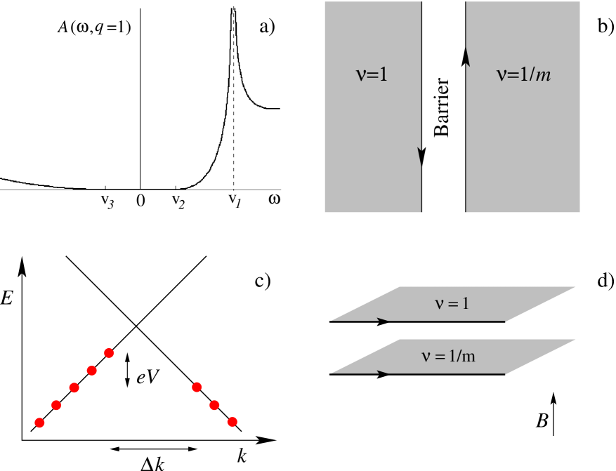
Figure 1: a) The electron spectral function in the reconstructed edge has singularities on the lines $\omega=v_{i}q$ that correspond to the edge excitation modes. The singularity at $\omega=v_{1}q$ is a divergence, and is the remnant of the $\delta$-peak in the unreconstructed edge. The spectral function vanishes for $v_{3}q<\omega<v_{2}q$ (e.g. for $q>0$) due to kinematic constrains. Shown is the case of the filling fraction $\nu=1/3$. b) The setup for the counter-propagating edge modes consists of $\nu=1$ and reconstructed $\nu=1/m$ states separated by a barrier which is uniform along the edges. Magnetic field is pointing into the page. c) The structure of the energy dispersion in the vicinity of the barrier for the case of counter-propagating edge modes (see text for details). d) The double-layer structure with the co-propagating edge modes.

The signatures of edge reconstruction in the spectral function are best observed in the so-called momentum-resolved tunneling experiments. [7, 8] In these experiments, the electron tunneling into the edge occurs across a barrier which is extended and homogeneous along the edge of the FQHE system, and so the electron’s momentum along the edge is conserved. First, we consider the simplest possible case of tunneling from the (un-reconstructed) edge of the QHE at the filling fraction $\nu=1$. The setup and the structure of energy levels under these conditions are shown in Figs. 1.b,c. The energy $E$ of the states is plotted as a function of momentum $k$ along the two parallel edges. The two straight lines in Fig. 1.c correspond to single electron dispersion on the two sides of the barrier. We shall treat tunneling using Fermi golden rule. Finally, we neglect the interaction between the edge modes on the opposite sides of the barrier, while the intra-edge interactions are taken into account by strong renormalization of the (charged) mode velocities.

There are two parameters that one can control: bias voltage $V$ and magnetic field $B$; $eV$ sets the difference between the Fermi energies on the two sides of the barrier, while the difference between the two Fermi momenta $\Delta k\propto B-B_{0}$, where $B_{0}$ is the strength of the magnetic field at which, in the absence of bias, the Fermi energy lies exactly at the dispersion lines crossing point. Below, we shall rescale $B$ so that $\Delta k=B-B_{0}$.

Within our approximations, the tunneling current is:

$$I(V,B) \propto \int A_{1}(\omega_{1},q_{1})A_{2}(\omega_{2},q_{2})[f(\omega_{1})-f(\omega_{2})]$$ (7)

$$\times\delta(eV+\omega_{1}-\omega_{2})\delta(B-B_{0}-q_{1}-q_{2}).$$

Here, $A_{1}=\delta(\omega-v_{F}q)$ is the spectral function of the $\nu=1$ edge with the Fermi velocity $v_{F}$, and $A_{2}$ is the spectral function of the reconstruted edge. $f(\omega)$ is the Fermi distribution step function.

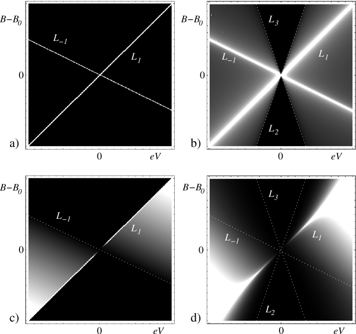
Figure 2: Differential conductance $dI/dV$ as a function of bias voltage $V$ and magnetic field $B$ for momentum-resolved tunneling from a counter-propagating unreconstructed $\nu=1$ edge to: a) unreconstructed $\nu=1$ edge; b) reconstructed $\nu=1$ edge; c) unreconstructed $\nu=1/3$ edge; d) reconstructed $\nu=1/3$ edge. Plotted is the derivative of the result in Eq. (7). Parameters are: $v_{1}=1$, $v_{2,3}=\pm 1/3$, $v_{F}=2$, $\alpha_{1}=m=\nu^{-1}$, $\alpha_{2,3}=0.2$. The dashed lines are guides to the eye and are defined as $L_{1,2,3}=\{eV=v_{1,2,3}(B-B_{0})\}$, $L_{-1}=\{eV=-v_{F}(B-B_{0})\}$. See text for details.

The result of the numerical evaluation of the differential conductance $dI/dV$ as a function of $V$ and $B-B_{0}$ is shown in Fig. 2. In general, the plot of $dI(V,B)/dV$ is very similar, but not identical to $A(\omega,q)$. In particular, both have 3 lines of singularities (marked by letters $L_{1,2,3}$ on the figure), one of them being a divergence. These lines correspond to the three edge excitation modes $\omega=v_{i}q$. Moreover, in the bow-tie region between $L_{2}$ and $L_{3}$ the differential conductance (as well as the current itself) is exactly zero. The reason for this is purely kinematic: In the region below the dispersion line of the slowest excitation in the system, one cannot satisfy the conservation of energy and momentum in tunneling.

The general structure of the spectral weight transfer provides a clear indication of the edge reconstruction. In particular, in the bow-tie regions between $L_{1}$ and $L_{2}$, and between $L_{3}$ and $L_{-1}$, $dI/dV$ is zero before reconstruction and finite after. We note, that the rise of $dI/dV$ in the region between $L_{3}$ and $L_{-1}$ is due to the appearance of a (neutral) edge mode that propagates in the direction opposite to the direction of the original edge mode.

Most of the results discussed above are also valid for the double-layer setup with co-propagating edge modes, shown in Fig. 1.d. The differential conductance in this case is plotted in Fig. 3. There is one crucial difference, however: In the co-propagating case there is a region (along $L_{-1}$) of negative differential conductance; reconstruction is expected to progressively wash this region out.

Although we have concentrated on the case of edge reconstruction described by a single point $k_{0}$, the preceding discussion remains generally valid for multiple edge reconstruction as well. In that case, new lines of singularities appear, while $L_{2}$ and $L_{3}$ correspond to the two slowest excitation modes.

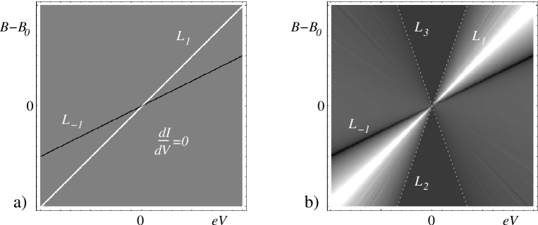
Figure 3: a) The $dI/dV$ for tunneling from unreconstructed $\nu=1$ to unreconstructed $\nu=1$ edge in the co-propagating case. $dI/dV=0$ everywhere except: $dI/dV>0$ on $L_{1}$, $dI/dV<0$ on $L_{-1}$. b) The $dI/dV$ for tunneling from unreconstructed $\nu=1$ to reconstructed $\nu=1$ edge in the co-propagating case. $dI/dV=0$ in the region between $L_{2}$ and $L_{3}$. Notation and parameters are the same as in Fig. 2, except $v_{F}=-2$ is used for this plot. Note that $dI/dV<0$ on $L_{-1}$.

Finally, we would like to comment on the role of the omitted $n\neq 0$ terms in Eq. (5). Apart from the factors $\exp ink_{0}x$, which trivially shift the momentum argument of the electron spectral function by $nk_{0}$, all terms with $n\neq 0$ are qualitatively similar to the $n=0$ term. Each of them produces a contribution to the Green’s function which is of the from Eq. (6), albeit with larger exponents $\alpha_{i}$. For that reason, all these terms make progressively less visible (but not necessarily unobservable) contributions to the spectral function.

We thank Matt Grayson, Woowon Kang, Leon Balents and Lloyd Engel for helpful discussions. This work was supported by NSF grant No. DMR-0225698.

References

- [1] X.-G. Wen, Int. J. Mod. Phys. B 6, 1711 (1992).
- [2] A. H. MacDonald, S. R. E. Yang, and M. D. Johnson, Aus. J. Phys. 46, 345 (1993).
- [3] C. Chamon and X.-G. Wen, Phys. Rev. B 49, 8227 (1994).
- [4] X. Wan, K. Yang, and E. H. Rezayi, Phys. Rev. Lett. 88, 056802 (2002).
- [5] X. Wan, E. H. Rezayi, and K. Yang, Phys. Rev. B 68, 125307 (2003).
- [6] K. Yang, Phys. Rev. Lett. 91, 036802 (2003).
- [7] W. Kang et al., Nature 403, 59 (2000); I. Yang et al., Phys. Rev. Lett. 92, 056802 (2004).
- [8] M. Huber et al., cond-mat/0309221; work in preparation.
- [9] U. Zülicke, E. Shimshoni, and M. Governale, Phys. Rev. B 65, 241315(R) (2002).
- [10] O. Heinonen and S. Eggert, Phys. Rev. Lett. 77, 358 (1996).
- [11] D. Carpentier, C. Peça, and L. Balents, Phys. Rev. B 66 153304 (2002).