Electronic Mechanism for the Coexistence of Ferroelectricity and Ferromagnetism

Abstract

We study the strong coupling limit of a two-band Hubbard Hamiltonian that also includes an inter-orbital on-site repulsive interaction $U_{ab}$. When the two bands have opposite parity and are quarter filled, we prove that the ground state is simultaneously ferromagnetic and ferroelectric for infinite intra-orbital Coulomb interactions $U_{aa}$ and $U_{bb}$. We also show that this coexistence leads to a singular magnetoelectric effect.

Introduction. The interplay between order parameters of different nature opens the door for designing new multifunctional devices whose properties can be manipulated with more than one physical field. For instance, the spin and orbital electronic degrees of freedom can order individually or simultaneously producing different phases. In particular, orbital ordering can produce symmetry-breaking states like orbital magnetism, ferroelectricity (FE), quadrupolar electric or magnetic ordering, and other multipolar orderings. The magnetoelectric multiferroics, such as $R$(Fe,Mn)O₃ Wang03 ; Kimura03 ; Lottermoser04 ; Aken04 ; Kimel05 and $R$Mn₂O₅ Hur04 ; Hur04_prl , are real examples of materials that combine distinct useful properties within a single system. Recent studies of these multiferroic materials have revived interest in the magnetoelectric effect, i.e., the induction of polarization with an applied magnetic field and magnetization with an applied electric field. To date, materials that exhibit both ferromagnetism (FM) and FE are rare Ederer04 because the transition metal ion of typical perovskite ferroelectrics is in a nonmagnetic $d^{0}$ electronic configuration. Therefore, it is essential to explore alternative routes to the coexistence of the FM and FE Ederer04 ; Efremov04 ; Ederer05 .

Different mechanisms for FE involving electronic degrees of freedom have been proposed. There are those in which FE results from bond ordered states induced either by electron-phonon coupling (Peierls instability) Littlewood79 or by pure electron-electron Coulomb interactions Armando04 . In these cases, the ferroelectric state is clearly nonmagnetic due to the singlet nature of the covalent bonds. In contrast, considering a system of interacting spinless fermions with two atomic orbitals of opposite inversion symmetry (say the $d$ and $f$ orbitals), Portengen et al. Portengen predicted that permanent electric dipoles are induced by spontaneous $d-f$ hybridization when particle-hole pairs (excitons) undergo a Bose-Einstein condensation. This result was confirmed in the strong coupling limit of an extended Falicov-Kimball spinless fermion model where both bands are dispersive Batista02 . It was also confirmed numerically in the intermediate coupling regime by using a constrained path Monte Carlo approach Batista04 .

The critical question that emerges is: How do FE and magnetism interplay when real electrons, instead of spinless fermions, are considered? In this Letter, we answer this question, proving that the mechanism proposed by Portengen et al. Portengen can coexist with magnetically ordered states. In this case, the single electron occupying the effective (say $d-f$ hybridized) orbital simultaneously provides an electric and a magnetic dipole moment, and the Coulomb repulsion is sufficient to generate a strong coupling between both of them.

We start from a two-band Hubbard Hamiltonian that includes an inter-orbital on-site repulsive interaction $U_{ab}$. Like in the spinless fermion case, this interaction provides the “glue” for the formation of excitons. At quarter filling and in the strong coupling limit, we map the low energy spectrum of the two-band Hubbard model, $H$, into an effective spin-pseudospin Hamiltonian, $H_{\rm eff}$, where the pseudospin represents the orbital degree of freedom. We prove that in the limit of large intra-orbital repulsive interactions $U_{aa},U_{bb}\rightarrow\infty$, $H_{\rm eff}$ has a ferromagnetic ground state that can be partially or fully saturated. By combining this result with the previous analysis for spinless fermions Batista02 ; Batista04 ; Wei03 , we show that FM and FE coexist, and a divergent magnetoelectric is demonstrated using the SO(4) symmetry of $H$. Our conclusions are reinforced by a semi-classical and a numerical computation of the zero temperature ($T=0$) phase diagram of $H$ that goes beyond the limiting case $U_{aa},U_{bb}\rightarrow\infty$.

Hamiltonian. We consider a two-band Hubbard model with a local inter-band Coulomb interaction $U_{ab}$ on a $D$-dimensional hypercubic lattice note :

$$H = \sum_{{\bf i},\eta,\nu,\nu^{\prime},\sigma}\!\!t_{\nu\nu^{\prime}}(f^{\dagger}_{\bf i\nu\sigma}f^{\;}_{{\bf i+{\hat{e}}_{\eta}}\nu^{\prime}\sigma}+f^{\dagger}_{{\bf i+{\hat{e}}_{\eta}}\nu^{\prime}\sigma}f^{\;}_{\bf i\nu\sigma})$$ (1)

$$+ \sum_{\bf i}U_{ab}n^{a}_{\bf i}n^{b}_{\bf i}+\sum_{\bf i,\nu}U_{\nu\nu}n^{\nu}_{\bf i\uparrow}n^{\nu}_{\bf i\downarrow}+\sum_{{\bf i},\nu}\epsilon_{\nu}n^{\nu}_{\bf i},$$

where $\eta=\{x,y,z,...\}$, $\nu=\{a,b\}$, $n^{\nu}_{\bf i\sigma}=f^{\dagger}_{\bf i\nu\sigma}f^{\;}_{\bf i\nu\sigma}$, $n^{\nu}_{\bf i}=\sum_{\sigma}n^{\nu}_{\bf i\sigma}$ and $n_{\bf i}=\sum_{\nu}n^{\nu}_{\bf i}$. Since the two orbitals, $a$ and $b$, have opposite parity under spatial inversion, the inter-band hybridization term must be odd under this operation: $t_{ab}=-t_{ba}$. In addition, the intra-band hoppings $t_{aa}$ and $t_{bb}$ will have opposite signs in general. The local spin and pseudospin operators are given by the expressions:

$$s^{\mu}_{\bf i\nu}=\frac{1}{2}\sum_{\alpha\alpha^{\prime}}f^{\dagger}_{\bf i\nu\alpha}{\sigma}^{\mu}_{\alpha\alpha^{\prime}}f^{\;}_{\bf i\nu\alpha^{\prime}},\;\;\tau^{\mu}_{\bf i\sigma}=\frac{1}{2}\sum_{\nu\nu^{\prime}}f^{\dagger}_{\bf i\nu\sigma}{\sigma}^{\mu}_{\nu\nu^{\prime}}f^{\;}_{\bf i\nu^{\prime}\sigma},$$ (2)

where ${\sigma}^{\mu}$ are the Pauli matrices with $\mu=\{x,y,z\}$. The total spin and pseudospin per site are: $s^{\mu}_{\bf i}=\sum_{\nu}s^{\mu}_{\bf i\nu}$ and $\tau^{\mu}_{\bf i}=\sum_{\sigma}\tau^{\mu}_{\bf i\sigma}$. The pseudospin component $\tau_{x}$ is proportional to the on-site hybridization. Since the the orbitals $a$ and $b$ have opposite parity, the local electric dipole moment is ${\bf p}_{\bf i}={\bm{\mu}}\tau^{x}_{\bf i}$, where ${\bm{\mu}}$ is the dipole matrix element between the $a$ and $b$ orbitals Batista02 ; Batista04 .

Symmetry is a useful concept for describing the coexistence of different order parameters.Ortiz04 For $t_{aa}=\pm t_{bb}$, $t_{ab}=t_{ba}=0$, $\epsilon_{a}-U_{aa}/2=\epsilon_{b}-U_{bb}/2$, and $U_{aa}=U_{ab}=U_{bb}$, $H$ is invariant under a U(1)$\otimes$SU(4) symmetry group. The U(1) symmetry corresponds to the conservation of the total number of particles. The generators of the SU(4) symmetry group are the three components of the total spin $s^{\mu}_{T}=\sum_{\bf i}s^{\mu}_{\bf i}$ and pseudospin $\tau^{\mu}_{T}=\sum_{\bf i}{\tau}^{\mu}_{\bf i}$ plus the nine operators:

$$\pi^{\mu\mu^{\prime}}=\frac{1}{2}\sum_{{\bf i},\alpha\nu\alpha^{\prime}\nu^{\prime}}f^{\dagger}_{{\bf i}\nu\alpha}{\sigma}^{\mu}_{\nu\nu^{\prime}}{\sigma}^{\mu}_{\alpha\alpha^{\prime}}f^{\;}_{{\bf i}\nu^{\prime}\alpha^{\prime}}.$$ (3)

The total spin is conserved for any set of parameters. If we just impose the condition $t_{ab}=t_{ba}=0$, the symmetry group of $H$ is reduced to the the subgroup U(1)$\times$U(1)$\times$SO(4). The six generators of the SO(4) group are the three components of total spin $s^{\mu}_{T}$ and the three operators $\pi^{z\mu}$. This symmetry arises from separate total spin and charge conservation of each band, as the two bands are only coupled by the Coulomb interaction $U_{ab}$. The symmetry operators $s^{\mu}_{T}\pm\pi^{z\mu}$ are the generators of global spin rotations on each individual band (with the $+$ sign for the $a$ band and the $-$ sign for the $b$ band).

Strong Coupling Limit. We will consider from now on the quarter filled case $n_{a}+n_{b}=1$, where $n_{a}$ and $n_{b}$ are the particle densities of the bands $a$ and $b$. When $U_{aa},U_{bb},U_{ab}\gg|t_{\nu\nu^{\prime}}|$, the low energy spectrum of $H$ can be mapped to an effective spin-pseudospin Hamiltonian by means of a canonical transformation that eliminates the linear terms in $t_{\nu\nu^{\prime}}$:

$$H {}_{\!\!\!\!\!\rm eff}=\!\sum_{{\bf i},\eta}[\sum_{\mu}J_{\mu}{\tau^{\mu}_{\bf i}}{\tau^{\mu}_{{\bf i}+{\bf e}_{\eta}}}+J_{xz}({\tau^{z}_{\bf i}}{\tau^{x}_{{\bf i}+{\bf e}_{\eta}}}-{\tau^{x}_{\bf i}}{\tau^{z}_{{\bf i}+{\bf e}_{\eta}}})]H^{H}_{{\bf i},\eta}$$

$$+ \!\!\!\sum_{{\bf i},\eta}{[}\frac{J_{0}}{2}+J_{1}(\tau^{z}_{\bf i}+\tau^{z}_{{\bf i}+{\bf e}_{\eta}})-J_{2}(\tau^{x}_{\bf i}-\tau^{x}_{{\bf i}+{\bf e}_{\eta}}){]}(H^{H}_{{\bf i},\eta}-\frac{1}{2})$$

$$+ \!\!\!\sum_{{\bf i},\eta}[J^{\prime}_{z}\tau^{z}_{\bf i}\tau^{z}_{{\bf i}+{\bf e}_{\eta}}+J^{\prime}_{xz}({\tau^{z}_{\bf i}}{\tau^{x}_{{\bf i}+{\bf e}_{\eta}}}-{\tau^{x}_{\bf i}}{\tau^{z}_{{\bf i}+{\bf e}_{\eta}}})]+\sum_{\bf i}B_{z}\tau^{z}_{\bf i},$$

where $H^{H}_{{\bf i},\eta}={\bf s_{i}}\cdot{\bf s_{{\bf i}+{\bf e}_{\eta}}}+\frac{1}{4}$ and

$$J_{z} = \frac{4(t_{bb}^{2}-t_{ab}^{2})}{U_{bb}}+\frac{4(t_{aa}^{2}-t_{ab}^{2})}{U_{aa}},$$

$$J_{x} = \frac{8(t_{bb}t_{aa}-t_{ab}^{2})}{U_{ab}},J_{y}=\frac{8(t_{bb}t_{aa}+t_{ab}^{2})}{U_{ab}},$$

$$J_{xz} = 4t_{ab}[\frac{(t_{aa}+t_{bb})}{U_{ab}}-\frac{t_{aa}}{U_{aa}}-\frac{t_{bb}}{U_{bb}}]$$

$$J_{0} = \frac{2(t_{bb}^{2}+t_{ab}^{2})}{U_{bb}}+\frac{2(t_{aa}^{2}+t_{ab}^{2})}{U_{aa}},J_{1}=\frac{2t_{bb}^{2}}{U_{bb}}-\frac{2t_{aa}^{2}}{U_{aa}},$$

$$J_{2} = 2t_{ab}[\frac{(t_{aa}-t_{bb})}{U_{ab}}+\frac{t_{aa}}{U_{aa}}-\frac{t_{bb}}{U_{bb}}]$$

$$J^{\prime}_{z} = \frac{2(t_{aa}^{2}+t_{bb}^{2}-2t_{ab}^{2})}{U_{ab}}-\frac{J_{z}}{2},$$

$$J^{\prime}_{xz} = 2t_{ab}[\frac{(t_{aa}+t_{bb})}{U_{ab}}+\frac{t_{aa}}{U_{aa}}+\frac{t_{bb}}{U_{bb}}],$$ (4)

and $B_{z}=\epsilon_{a}-\epsilon_{b}+(U_{bb}-U_{aa})/2$. In this limit, because the double-occupancy is forbidden in the low energy Hilbert space of $H_{\rm eff}$, both ${\bf s}_{\bf i}$ and ${\bf\tau}_{\bf i}$ belong to the $S=1/2$ representation of the su(2) algebra. The first two terms of $H_{\rm eff}$ couple the spin and the orbital degrees of freedom. As usual, the Heisenberg antiferromagnetic interaction, $H^{H}_{{\bf i},\eta}$, is a direct consequence of the Pauli exclusion principle. On the other hand, the anisotropic Heisenberg-like pseudospin-pseudospin interaction reflects the competition between an excitonic crystallization or staggered orbital ordering (SOO) induced by the Ising term, and a Bose-Einstein condensation of excitons induced by the $XY$-term Batista02 ; Wei03 . The first term of $H_{\rm eff}$ shows explicitly that the amplitude of the excitonic kinetic energy (or $XY$-pseudospin) term gets maximized when the excitons are in a fully polarized ferromagnetic spin state. However, antiferromagnetism (AF) is clearly favored by the second term.

Large $U_{aa}$, $U_{bb}$ limit. We will first prove that there are partially and fully polarized ferromagnetic ground states of $H_{\rm eff}$ in the limit of $U_{aa}$, $U_{bb}\rightarrow\infty$ and $t_{ab}=0$, and that the total spin or magnetization $s_{T}$ take the values $\tau^{z}_{T}\leq s_{T}\leq N/2$. After proving this result, we will show that these ferromagnetic solutions are also ferroelectric for $B^{c1}_{z}\leq B_{z}<B^{c2}_{z}$ and, using the SO(4) symmetry, we will derive an exact expression for ground state electric polarization as a function of the magnetization.

Since $J_{0}$ and $J_{1}$ vanish in this limit, $H_{\rm eff}$ is reduced to:

$${\bar{H}}_{\rm eff} = \sum_{\langle\bf i,j\rangle}[{J^{\prime}_{z}}{\tau^{z}_{i}}{\tau^{z}_{j}}+J_{\perp}(\tau^{x}_{\bf i}\tau^{x}_{\bf j}+\tau^{y}_{\bf i}\tau^{y}_{\bf j})H^{H}_{\bf i,j}]+B_{z}\sum_{\bf i}\tau^{z}_{\bf i},$$

where the angular brackets indicate that the sum is over nearest-neighbors, $J_{\perp}=J_{x}=J_{y}$, and $H^{H}_{\bf i,j}={\bf s_{i}}\cdot{\bf s_{j}}+\frac{1}{4}$. To prove our statement we will use a basis of eigenstates of the local operators $\tau^{z}_{\bf i}$ and $s^{z}_{\bf i}$: $\{|\tau^{z}_{1}...\tau^{z}_{N}\rangle\otimes|s^{z}_{1}...s^{z}_{N}\rangle\}$ where $N$ is the total number of sites. The off-diagonal matrix elements of ${\bar{H}}_{\rm eff}$

$$\langle s^{\prime z}_{N}...s^{\prime z}_{1}|\otimes\langle\tau^{\prime z}_{N}...\tau^{\prime z}_{1}|{\bar{H}}_{\rm eff}|\tau^{z}_{1}...\tau^{z}_{N}\rangle\otimes|s^{z}_{1}...s^{z}_{N}\rangle=$$

$$2J_{\perp}\sum_{\langle\bf i,j\rangle}\langle\tau^{\prime z}_{N}...\tau^{\prime z}_{1}|H^{xy}_{\bf i,j}|\tau^{z}_{1}...\tau^{z}_{N}\rangle\langle s^{\prime z}_{N}...s^{\prime z}_{1}|H^{H}_{\bf i,j}|s^{z}_{1}...s^{z}_{N}\rangle$$ (5)

are non-positive because $J_{\perp}<0$, and the matrix elements of $H^{xy}_{\bf i,j}=\tau^{x}_{\bf i}\tau^{x}_{\bf j}+\tau^{y}_{\bf i}\tau^{y}_{\bf j}$ and $H^{H}_{\bf i,j}$ are explicitly non-negative. According to the generalized Perron’s theorem (see for instance Ref. Horn ), there is one ground state of ${\bar{H}}_{\rm eff}$,

$$|\Psi^{g}\rangle=\sum_{\{\tau^{z}\}}|\tau^{z}_{1}...\tau^{z}_{N}\rangle\otimes\sum_{\{s^{z},s^{z}_{T}=0\}}a_{\{\tau^{z}\},\{s^{z}\}}|s^{z}_{1}...s^{z}_{N}\rangle,$$ (6)

such that all the amplitudes $a_{\{\tau^{z}\},\{s^{z}\}}$ are non-negative ( $\{\tau^{z}\}$ and $\{s^{z}\}$ denote all the possible configurations of $\tau^{z}_{\bf i}$ and $s^{z}_{\bf i}$). We can rewrite $|\Psi^{g}_{s^{z}_{T}=0}\rangle$ in the following way:

$$|\Psi^{g}\rangle=\sum_{\{\tau^{z}\}^{\prime}}b_{\{\tau^{z}\}}|\tau^{z}_{1}...\tau^{z}_{N}\rangle\otimes|\Phi\{\tau^{z}\}\rangle,$$ (7)

with

$$|\Phi\{\tau^{z}\}\rangle = \frac{1}{b_{\{\tau^{z}\}}}\sum_{\{s^{z},s^{z}_{T}=0\}}a_{\{\tau^{z}\},\{s^{z}\}}|s^{z}_{1}...s^{z}_{N}\rangle,$$

$${b_{\{\tau^{z}\}}} = \sqrt{\sum_{\{s^{z},s^{z}_{T}=0\}}a^{2}_{\{\tau^{z}\},\{s^{z}\}}}.$$ (8)

The set ${\{\tau^{z}\}^{\prime}}$ corresponds to all the configurations of the $\tau^{z}_{\bf i}$ variables such that ${b_{\{\tau^{z}\}}}>0$. Note that each spin state $|\Phi\{\tau^{z}\}\rangle$ is normalized and $\sum_{\bf i}b^{2}_{\{\tau^{z}\}}=1$ because $|\Psi^{g}\rangle$ is also normalized. The ground state energy of ${\bar{H}}_{\rm eff}$ is :

$$\langle\Psi^{g}|{\bar{H}}_{\rm eff}|\Psi^{g}\rangle=\langle\Psi^{g}|\sum_{\langle\bf i,j\rangle}{J_{z}}{\tau^{z}_{i}}{\tau^{z}_{j}}+B_{z}\sum_{\bf i}\tau^{z}_{\bf i}|\Psi^{g}\rangle+$$

$$2J_{\perp}\sum_{\langle\bf i,j\rangle}\sum_{\{\tau^{z},\tau^{\prime z}\}^{\prime}}b_{\{\tau^{z}\}}b_{\{\tau^{\prime z}\}}\langle\tau^{\prime z}_{N}...\tau^{\prime z}_{1}|H^{xy}_{\bf i,j}|\tau^{z}_{1}...\tau^{z}_{N}\rangle\times$$

$$\langle\Phi\{\tau^{\prime z}\}|H^{H}_{\bf i,j}|\Phi\{\tau^{z}\}\rangle.$$ (9)

$H^{H}_{\bf i,j}$ is a bounded operator with eigenvalues $\pm 1/2$. Therefore $\langle\Phi\{\tau^{\prime z}\}|H^{H}_{\bf i,j}|\Phi\{\tau^{z}\}\rangle\leq 1/2$ and the equality holds for any pair of nearest-neighbor sites $({\bf i,j})$ if $|\Phi\{\tau^{z}\}\rangle=|s^{z}_{T},s_{T}=N/2\rangle$ where $|s^{z}_{T},s_{T}=N/2\rangle$ is the state with maximum total spin (fully polarized) and $\sum_{\bf i}s^{z}_{\bf i}=s^{z}_{T}$. Hence, expression (9) is minimized for the fully polarized spin configuration which means that there is family of ground states $|\Psi^{g}\rangle$ that have maximum total spin $s_{T}$ and different values of $s^{z}_{T}$:

$$|\Psi^{g}\rangle=\sum_{\{\tau^{z}\}^{\prime}}b_{\{\tau^{z}\}}|\tau^{z}_{1}...\tau^{z}_{N}\rangle\otimes|s^{z}_{T},s_{T}=N/2\rangle.$$ (10)

This proves that there is a fully polarized ferromagnetic ground state of ${\bar{H}}_{\rm eff}$. Note the proof is valid in any dimension and is also valid for non-bipartite lattices. When we restrict ${\bar{H}}_{\rm eff}$ to the subspace with maximum total spin ($s_{T}=N/2$), the operator $({\bf S_{i}}\cdot{\bf S_{j}}+\frac{1}{4})$ is replaced by $1/2$ and the restricted Hamiltonian ${\bar{H}}^{FM}_{\rm eff}$ becomes exactly the same as the one obtained in Ref. Batista02 for the strong coupling limit of a spinless extended Falicov-Kimball model Falicov . As shown in Ref. Batista02 ; Wei03 , the quantum phase diagram of ${\bar{H}}^{FM}_{\rm eff}$ contains a ferroelectric phase for $B^{c1}_{z}\leq B_{z}<B^{c2}_{z}$, i.e., for a non-zero value of $\tau^{z}_{T}$.

The SO(4) symmetry of ${\bar{H}}_{\rm eff}$ implies that the ground state degeneracy is higher than the $2s_{T}+1=N+1$ multiplet obtained from the global SU(2) spin rotations. Ground states with different total spin can also be obtained by making different global spin rotations for the bands $a$ and $b$. The spins of each individual band will remain fully polarized under these transformations, but the relative orientation between spins of different bands will change. In particular, the minimum total spin will occur when spins in different bands are “anti-aligned”, i.e., $s_{T}=\tau^{z}_{T}$. This implies that the total spin of the ground state can take the values: $\tau^{z}_{T}\leq s_{T}\leq N/2$.

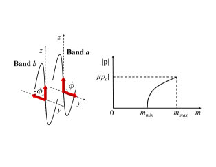
Figure 1: Evolution of the magnetization (arrows) on each band under the SO(4) transformation $U(\phi)$. The ${\bf P}$ vs ${\bf m}$ plot shows the change of the electric dipole moment when the total magnetization evolves from the minimum value, obtained for $\phi=\pi/2$, to the maximum value $m(\phi=0)=1/2$.

To derive the magneto-electric effect, we define $|\chi\rangle$ as the fully polarized ferromagnetic and ferroelectric state obtained for $B^{c1}_{z}\leq B_{z}<B^{c2}_{z}$. Then, the average magnetization and electric dipole moment per site, $m$ and ${\bf p}$, are given by:

$$m=\frac{\sqrt{\langle\chi|{\bf s}^{2}_{T}|\chi\rangle}}{N}=\frac{1}{2}\sqrt{1+\frac{2}{N}},\;\;\;{\bf p}={\bm{\mu}}p_{0},$$ (11)

where $p_{o}=\langle\chi|\tau^{x}_{T}|\chi\rangle/N$. A given ground state in the SO(4) multiplet can expressed as $|g_{u}\rangle=U|\chi\rangle$, where $U$ is an element of the SO(4) group. In particular, choosing the set of transformations $U(\phi)=e^{i\phi\sum_{\bf j}(S^{x}_{{\bf j}a}-S^{x}_{{\bf j}b})}$ we get for ${\bf p}(\phi)={\bm{\mu}}\langle g_{u(\phi)}|\tau^{x}_{T}|g_{u(\phi)}\rangle/N$ and $m(\phi)=\sqrt{\langle g_{u(\phi)}|{\bf s}^{2}_{T}|g_{u(\phi)}\rangle}/N$:

$$m(\phi)= = \frac{1}{2}\sqrt{1-4n_{a}n_{b}\sin^{2}{\!\!\phi}+\frac{2}{N}},$$

$${\bf p}(\phi) = {\bm{\mu}}p_{o}\cos{\phi},$$ (12)

where we have used that ${\bf s}_{T}={\bf s}_{aT}+{\bf s}_{bT}$ and that $U(\phi)$ rotates the vectors ${\bf s}_{aT}$ and ${\bf s}_{bT}$ around the $x$-axis by angles $\phi$ and $-\phi$ respectively. For the second relation, we have used that:

$$U^{\dagger}(\phi)\tau^{x}_{T}U^{\;}(\phi)=\cos{\phi}\;\tau^{x}_{T}-\sin{\phi}\;\pi^{yx},$$ (13)

and $\langle\chi|\pi^{yx}|\chi\rangle=0$. For $\phi=\pi/2$, the magnetization of the $a$ and $b$ bands have opposite sign (see Fig.1) and the total magnetization per site is minimized: $m_{min}=m(\pi/2)=|n_{a}-n_{b}|/2$ (we have taken the thermodynamic limit $N\rightarrow\infty$). The electric polarization can be expressed as a function of $m$ by combining Eqs. (12):

$$|{\bf p}|=2|{\bm{\mu}}p_{0}|\frac{\sqrt{m^{2}-m^{2}_{min}}}{\sqrt{1-4m_{min}^{2}}}.$$ (14)

The electric dipole moment is zero for $m=m_{min}$ and it increases as $\sqrt{m-m_{min}}$ implying that the derivative $d|P|/dm$ diverges at $m=m_{min}$ as $1/\sqrt{m-m_{min}}$. This important result shows that the interplay between the spin and the orbital degrees of freedom can produce an enormous magneto-electric effect (see Fig. 1).

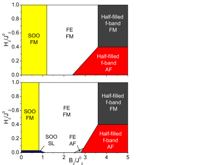
Figure 2: Zero temperature phase diagram of the two dimensional version of $H_{\rm eff}$ plus a Zeeman term $H_{z}s^{z}_{T}$ computed in the spin-wave approximation (top) and by exact diagonalization of a $4\times 4$ cluster (bottom). The parameter values are $J_{0}=0.2J_{z}^{0}$, $J_{x}=J_{y}=-1.6J_{z}^{0}$, $J_{1}=-0.1J_{z}^{0}$ and $J_{z}^{0}=J^{\prime}_{z}+J_{z}/2$.

It is important to verify the stability of the coexisting ferroelectric and ferromagnetic phases away from the limit we have considered above. For this purpose, we computed the $T=0$ diagram of the two dimensional version of $H_{\rm eff}$ plus a Zeeman term, $H_{z}s^{z}_{T}$, in a spin-wave approximation (top of Fig. 2) and by exact diagonalization of a $4\times 4$ cluster (bottom of Fig. 2). In this case, the values of of $U_{aa}$ and $U_{bb}$ are finite ($J_{0}=0.2J_{z}^{0}$), and the coexistence of FM and FE obtained for $H_{z}=0$ and $B^{c1}_{z}\leq B_{z}<B^{c2}_{z}$ is still present (see Fig. 2). For $B_{z}<B^{c1}_{z}$ and $H_{z}=0$, the spin-wave phase diagram exhibits coexistence of FM and SOO Batista02 . The FM ordering is replaced by a spin liquid (short ranged spin-spin correlations) in the phase diagram computed by exact diagonalization indicating that quantum fluctuations play a major role in that regime of parameters. As expected, for large enough $B_{z}$ the system becomes an antiferromagnetic Mott insulator (one band is a half-filled and the other one is empty). The exact diagonalization shows again that quantum fluctuations generate an intermediate phase between the FE-FM state and the Mott insulator in which FE and AFM coexist (see bottom of Fig. 2). For high values of $H_{z}$, the system is fully polarized and the both $T=0$ phase diagrams coincide with the one obtained in Ref. Batista02 .

The ferromagnetic state can be further stabilized by the inclusion of the ferromagnetic on-site inter-orbital exchange interaction. For example, the intra-atomic $4f-5d$ exchange interaction is about 0.2 eV in EuB₆ Kunes ; Li . The other important aspect to consider is the role of a finite inter-band hybridization $t_{ab}$. Exact diagonalization results Wei show that the lowest total spin ground state, $s_{T}=\tau^{z}_{T}$ or $m=m_{min}$, is the one stabilized after the inclusion of a small $t_{ab}$ term. According to Eq.(14), this unsaturated ferromagntic state gives rise to a divergent magnetoelectric effect. In this situation, a small increase in the magnetization produced by an applied magnetic field will generate a large increase of the electric dipole moment in the way depicted in Fig. 1.

In summary, we have shown that the electron-electron Coulomb interaction can produce coexisting FM and FE. Both phases arise simultaneously from the condensation of excitons or particle-hole pairs that exist in two bands with opposite parity under spatial inversion. The coexistence requires the presence of large intra-orbital Coulomb interactions to reduce the strength of the antiferromagnetic interaction. We have also shown that the coexistence of FE and FM leads to a divergent magnetoelectric effect. In the proximity of the ferroelectric-ferromagnetic instability, a small magnetic field can produce an enormous change in the electric polarization.

We thank W. E. Pickett and J. Kuneš for pointing out Ref. Li . LANL is supported by US DOE under Contract No. W-7405-ENG-36. BNL is supported by US DOE under Contract No. DE-AC02-98CH1-886.

References

• (1) J. Wang et al., Science 299, 1719 (2003).
• (2) T. Kimura et al., Nature 426, 55 (2003).
• (3) T. Lottermoser et al., Nature 430, 541 (2004).
• (4) B. B. Van Aken et al., Nature Materials 3, 164 (2004).
• (5) A. V. Kimel et al., Nature 435, 655 (2005).
• (6) N. Hur et al., Nature 429, 392 (2004).
• (7) N. Hur et al., Phys. Rev. Lett. 93, 107207 (2004).
• (8) C. Ederer and N. A. Spaldin, Nature Materials 3, 849 (2004).
• (9) D. V. Efremov, J. Van Den Brink, and D. I. Khomskii, Nature Materials 3, 853 (2004).
• (10) C. Ederer and N. A. Spaldin, Phys. Rev. B 71, 060401(R) (2005); ibid. 71, 224103 (2005). P. Baettig and N. A. Spaldin, Appl. Phys. Lett. 86, 012505 (2005).
• (11) P. B. Littlewood and B. Heine, J. Phys. C: Solid State Phys. 12, 4431 (1979).
• (12) C. D. Batista and A. A. Aligia, Phys. Rev. Lett. 92, 246405 (2004); Phys. Rev. B 71, 125110 (2005).
• (13) T. Portengen, Th. Γ–streich and L. J. Sham, Phys. Rev. Lett. 76, 3384 (1996); Phys. Rev. 54, 17452 (1996).
• (14) C. D. Batista, Phys. Rev. Lett. 89, 166403 (2002).
• (15) C. D. Batista, J. E. Gubernatis, J. Bonča and H. Q. Lin, Phys. Rev. Lett. 92, 187601 (2004).
• (16) W. G. Yin et al., Phys. Rev. B 68, 075111 (2003).
• (17) This is the minimal Hamiltonian for studying the interplay between electronic ferroelectricity and magnetism. In real systems, the number of orbitals that lie close to the Fermi level after the crystal filed splitting can be higher than two.
• (18) C. D. Batista and G. Ortiz, Adv. in Phys. 53, 1 (2004).
• (19) R. A. Horn and C. R. Johnson, Matrix Analysis, (Cambridge University Press, 1985).
• (20) L. M. Falicov and J. C. Kimball, Phys. Rev. Lett. 22, 997 (1969).
• (21) Note that in the reduced Hilbert space of $H_{\rm eff}$ the operator $\pi^{z\mu}$ can be expressed as: Ο€z​μ=βˆ‘π’Ο„π’z​s𝐒μsuperscriptπœ‹π‘§πœ‡subscript𝐒subscriptsuperscriptπœπ‘§π’subscriptsuperscriptπ‘ πœ‡π’\pi^{z\mu}=\sum_{\bf i}\tau^{z}_{\bf i}s^{\mu}_{\bf i}.
• (22) W. G. Yin et al., to be published.
• (23) J. KuneΕ‘ and W. E. Pickett, Phys. Rev. B 69, 165111 (2004).
• (24) Hong-Shuo Li, Y. P. Li, and J. M. D. Coey, J. Phys.: Condens. Matter 3, 7277 (1991).