Quantum-to-classical correspondence in open chaotic systems

Abstract

We review properties of open chaotic mesoscopic systems with a finite Ehrenfest time $\tau_{\rm E}$. The Ehrenfest time separates a short-time regime of the quantum dynamics, where wave packets closely follow the deterministic classical motion, from a long-time regime of fully-developed wave chaos. For a vanishing Ehrenfest time the quantum systems display a degree of universality which is well described by random-matrix theory. In the semiclassical limit, $\tau_{\rm E}$ becomes parametrically larger than the scattering time off the boundaries and the dwell time in the system. This results in the emergence of an increasing number of deterministic transport and escape modes, which induce strong deviations from random-matrix universality. We discuss these deviations for a variety of physical phenomena, including shot noise, conductance fluctuations, decay of quasibound states, and the mesoscopic proximity effect in Andreev billiards.

1 Introduction

Technological advances of the past decade have made it possible to construct clean electronic devices of a linear size smaller than their elastic mean free path, but still much larger than the Fermi wavelength [1, 2, 3]. The motion of the electrons in these quantum dots is thus ballistic, and determined by an externally imposed confinement potential. On the classical level the dynamics can vary between two extremes, according to whether the confinement potential gives rise to integrable or chaotic motion [4, 5]. This classification is carried over to the quantum dynamics [6, 7, 8, 9], with most of the theoretical efforts focusing on the chaotic case. It has been conjectured [10, 11] that chaotic quantum dots fall into the same universality class as random disordered quantum dots. The latter exhibit a degree of universality which is well captured by random-matrix theory (RMT) [12, 13, 14]. Starting, e.g., from the scattering theory of transport [15, 16], RMT provides a statistical description, where the system’s scattering matrix is assumed to be uniformly distributed over one of Dyson’s circular ensembles [17, 18, 19]. This sole assumption allows to calculate transport quantities such as the average conductance, shot noise, and counting statistics, including coherent quantum corrections such as weak localization and universal conductance fluctuations [12, 13, 14]. RMT can also be extended to the energy dependence of the scattering matrix by linking it to a random effective Hamiltonian of Wigner’s Gaussian universality classes [14, 19, 20]. This allows to investigate quantum dynamical properties such as time delays and escape rates [21], as well as the density of states of normal-superconducting hybrid structures [22].

RMT assumes that all cavity modes are well mixed, hence, that the system displays well-developed wave chaos. Impurities serve well for this purpose, since s-wave scattering couples into all directions with the same strength. Indeed, RMT enjoys a well-based mathematical foundation for disordered systems [20, 23, 24]. In ballistic chaotic systems, the scattering is off the smooth boundaries, which is not directly diffractive in contrast to the scattering from an impurity. On the other hand, classical chaos is associated to a strong sensitivity of the dynamics to uncertainties in the initial conditions, which are amplified exponentially with time $\sim\exp(\lambda t)$ (where $\lambda$ is the Lyapunov exponent). Hence, there are little doubts that RMT also gives a correct description for ballistic systems where this sensitivity yields to well-developed wave chaos.

The precise conditions under which wave chaos emerges from classical chaos are however just being uncovered. Generically, RMT is bounded by the existence of finite time scales. In closed chaotic systems, for instance, spectral fluctuations are known to deviate from RMT predictions for energies larger than the inverse period of the shortest periodic orbit [11]. For transport through open chaotic systems, classical ergodicity clearly has to be established faster than the lifetime of an electron in the system. Accordingly, the dynamics should not allow for too many short, nonergodic classical scattering trajectories going straight through the cavity, or hitting its boundary only very few times [25]. This requires that the inverse Lyapunov exponent $\lambda^{-1}$ and the typical time $\tau_{\rm B}$ between bounces off the confinement are much smaller than the dwell time $\tau_{\rm D}$, hence $\lambda^{-1},\tau_{\rm B}\ll\tau_{\rm D}$. In practice, these conditions are fulfilled when the openings are much smaller than the linear system size $L$. RMT universality also requires that $\lambda^{-1}$, $\tau_{\rm B}$, and $\tau_{D}$ are smaller than the Heisenberg time $\tau_{\rm H}=h/\Delta$ (with $\Delta$ the mean level spacing). The condition $\tau_{\rm H}\gg\tau_{\rm B}$ guarantees that a large number of internal modes $M={\rm Int}[\tau_{\rm H}/\tau_{\rm B}]$ are mixed by the chaotic scattering (RMT is then independent of microscopic details of the ensemble [14]). The condition $\tau_{H}\gg\tau_{D}$ translates into a large total number of open scattering channels in all leads, $N_{\rm tot}={\rm Int}\,[\tau_{\rm H}/\tau_{\rm D}]$, such that details of the openings can be neglected. Together with the condition $\tau_{B}\ll\tau_{D}$, this implies $1\ll N_{\rm tot}\ll M$. The limit $M\to\infty$, $M/N_{\rm tot}={\rm const}$ is equivalent to the semiclassical limit of a small Fermi wave length $\lambda_{\rm F}/L\to 0$, all classical parameters being kept fixed. These requirements have been thoroughly investigated in the past [14, 24, 26].

More recently, following the seminal work of Aleiner and Larkin [27], it has become clear that a new time scale, associated to the quantum-to-classical correspondence of wave-packet dynamics (and in this sense, the validity of Ehrenfest’s theorem), also restricts the validity of the RMT of ballistic transport. This time scale $\tau_{\rm E}$, usually referred to as the Ehrenfest time, is roughly the time it takes for the chaotic classical dynamics to stretch an initially narrow wave packet, of Fermi wavelength $\lambda_{\rm F}$, to some relevant classical length scale ${\cal L}$ (cf. Fig. 1). Since the stretching $\propto\exp[\lambda t]$ is exponential in time, one has $\tau_{\rm E}\propto\lambda^{-1}\ln[{\cal L}/\lambda_{\rm F}]$ [28]. The Ehrenfest time poses a lower limit to the validity of RMT because wave chaos is associated to the splitting of wave packets into many partial waves, which then interfere randomly. In ballistic chaotic systems, the wave packet splitting is only established when initial quantum uncertainties blow up to the classical level. For shorter times, the quantum dynamics still bears the signatures of classical determinism, which is not captured by RMT.

When $\lambda_{\rm F}$ is decreased, all classical parameters being kept constant – the very same semiclassical limit purportedly required for RMT universality – $\tau_{\rm E}$ becomes parametrically larger than $\tau_{\rm B}$ and $\lambda^{-1}$, and indeed may start to compete with the dwell time $\tau_{\rm D}$. One may thus wonder what is left of the RMT universality of open systems, and more generally of quantum effects in that limit. Indeed, there are many instances where quantum-to-classical correspondence at finite $\tau_{\rm E}$ leads to strong deviations from the universal RMT behavior. Such deviations are not only of fundamental interest, but also provide practical mechanisms to suppress or accentuate quantum properties. This short review provides a survey of the current knowledge of the quantum-to-classical correspondence in open ballistic systems, focusing on the deviations from RMT due to a finite Ehrenfest time.

We start with a brief general classification of the Ehrenfest time for different physical situations such as transport, escape, and closed-system properties (section 2). We then turn our attention to three specific applications where deviations from RMT universality occur once the relevant Ehrenfest time is no longer negligible. First (section 3), we discuss transport properties in a two-terminal geometry. Quantum-to-classical correspondence is reflected in the distribution of the transmission eigenvalues, and results in the suppression of electronic shot noise and the breakdown of universality for sample-to-sample conductance fluctuations. Second (section 4), we discuss the decay modes (quasi-bound states) of the system. Escape routes faster than the Ehrenfest time give rise to highly localized, ballistically decaying quasi-bound states, while the density of long-lived quasi-bound states is renormalized according to a fractal Weyl law. Finally (section 5), we investigate the excitation spectrum of normal-metallic ballistic quantum dots coupled to an $s$-wave superconductor (the mesoscopic proximity effect). The presence of the superconducting terminal introduces a new dynamical process called Andreev reflection (charge-inverting retroreflection), which induces a finite quasiparticle lifetime and opens up a gap in the density of states around the Fermi energy. The size and shape of the gap show deviations from the RMT predictions when the Ehrenfest time is no longer negligible against the lifetime of the quasiparticle. Conclusions are presented in section 6.

Because of the slow, logarithmic increase of $\tau_{\rm E}\propto\ln M$ with the effective size $M$ of the Hilbert space, the ergodic semiclassical regime $\tau_{\rm E}\gtrsim\tau_{\rm D}$, $\lambda\tau_{\rm D}\gg 1$ is unattainable by standard numerical methods. The numerical results reviewed in this paper are all obtained for a very efficient model system, the open kicked rotator [29, 30, 31, 32], which we briefly describe in the Appendix.

2 Classification of Ehrenfest times

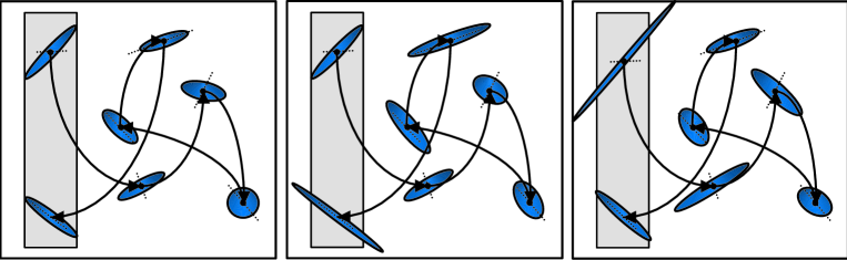
Figure 1: Sketch of the dynamics of a wave packet in the phase space of an open system. The left and middle panels apply to the case of transport. The initial wave packet is maximally stretched along the stable manifold without substantial leakage out of the shaded rectangular area, which represents an opening of the system. After five bounces the wave packet returns to the opening, now being elongated along the unstable manifold (dashed lines; the sketches neglect the bending of the manifolds). In the left picture, the transport Ehrenfest time $\tau_{\rm E}^{(2)}$ is larger than the dwell time $\tau_{\rm D}$. The returning wave packet still fits through the opening, with only minimal leakage. Hence, the particle leaves the system deterministically, as prescribed by the classical dynamics of the wave-packet center (dots). The middle picture corresponds to a more chaotic system (with larger Lyapunov exponent), resulting in $\tau_{\rm E}^{(2)}<\tau_{\rm D}$. The stretching is stronger and the wave packet is not fully transmitted. In the subsequent dynamics, the partially reflected wave components will interfere randomly, which gives rise to wave chaos. In the escape problem, the initial wave packet can be squeezed more closely to the stable manifold, and the associated Ehrenfest time $\tau_{\rm E}^{(1)}$ is larger than the transport Ehrenfest time. This is illustrated in the right panel.

The relevant Ehrenfest time depends on the physical situation at hand, but follows a very simple classification. Quantum-to-classical correspondence is maximized for wave packets that are initially elongated along the stable manifold of the classical dynamics, so that the dynamics first yields to compression, not to stretching (see Fig. 1). The initial extent of elongation along the stable manifolds is limited either by the linear width of the openings $W$, or the linear system size $L$, depending on whether the physical process requires injection into the system or not. In the same way, the final extent of the wave packet has to be compared to $W$ or $L$ depending on whether the physical process requires the particle to leave the system or not. For sufficiently ergodic chaotic dynamics ($\lambda^{-1}$, $\tau_{\rm B}\ll\tau_{\rm D}$, which implies $W\ll L$) and in the absence of sharp geometrical features (besides the presence of the openings), the resulting Ehrenfest time can be expressed by the three classical time scales and the Heisenberg time $\tau_{\rm H}$ [28, 33, 34]:

$$\tau_{\rm E}^{(n)}=\lambda^{-1}\ln\left[\frac{\tau_{\rm H}}{\tau_{\rm B}}\left(\frac{\tau_{\rm B}}{\tau_{\rm D}}\right)^{n}\right]\;\;\;;\;\;\;n=\left\{\begin{array}[]{cc}0&{\rm closed\;system},\\ 1&{\rm escape},\\ 2&{\rm transport}.\end{array}\right.$$ (1)

Here $n$ gives the number of passages through the openings associated to the physical process. Expression (1) holds for two-dimensional systems such as lateral quantum dots [1, 2, 3] or microwave cavities [9], as well as for the stroboscopic one-dimensional model systems often used in the numerical simulations ($\tau_{\rm B}$ is then the stroboscopic period; see the Appendix). Expression (1) also holds for three-dimensional systems (such as metallic grains) with two-dimensional openings when $\lambda$ is replaced by the sum of the two positive Lyapunov exponents.

The difference between the three Ehrenfest times can be attributed to the additional splitting of a wave packet into partially transmitted and partially reflected waves at each encounter with an opening. Transport involves two passages via the openings. The first passage, at injection, determines the initial spread of the associated wave packet. The Ehrenfest time is then obtained by comparing the final spread to the width of the opening at the second passage, where the electron leaves the system. This results in the transport Ehrenfest time $\tau_{\rm E}^{(2)}=\lambda^{-1}\ln[\tau_{\rm H}\tau_{\rm B}/\tau_{\rm D}^{2}]$. The same Ehrenfest time also affects the excitation spectrum of normal-metallic cavities which are coupled by the openings to an $s$-wave superconductor, for which the relevant physical process is the consecutive Andreev reflection of the two quasi-particle species at the superconducting terminal ($\tau_{\rm E}^{(2)}$ was actually first derived in that context [33]). In the escape problem, the electron is no longer required to originate from an opening. This lifts the restriction on the initial confinement of the wave packet and allows to squeeze it closer to the stable manifolds, as its elongation is not limited by the width of the opening but by the linear system size. Hence, the escape Ehrenfest time is larger than the transport Ehrenfest time by a factor $\tau_{\rm D}/\tau_{\rm B}$ in the logarithm: $\tau_{\rm E}^{(1)}=\lambda^{-1}\ln[\tau_{\rm H}/\tau_{\rm D}]$. This value is exactly in the middle of the transport Ehrenfest time $\tau_{\rm E}^{(2)}$ and the conventional Ehrenfest time $\tau_{\rm E}^{(0)}=\lambda^{-1}\ln[\tau_{\rm H}/\tau_{\rm B}]$ for closed systems [28], for which initial and final extents of the wave packet must be compared against the linear size of the system.

The semiclassical limit is achieved for $\tau_{\rm H}\to\infty$ while the classical time scales $\lambda^{-1}$, $\tau_{\rm B}$, and $\tau_{\rm D}$ are fixed. The Ehrenfest time then increases logarithmically with $\tau_{\rm H}/\tau_{\rm B}$, which is $\propto L/\lambda_{\rm F}$ for two dimensions and $\propto(L/\lambda_{\rm F})^{2}$ for three dimensions. In this paper, we will denote this limit by $M\to\infty$ while keeping $M/N_{\rm tot}$ fixed, where $M={\rm Int}[\tau_{\rm H}/\tau_{\rm B}]$ is the effective number of internal modes mixed by the chaotic scattering, and $N_{\rm tot}={\rm Int}[\tau_{\rm H}/\tau_{\rm D}]\ll M$ is the total number of open channels.

3 Quantum-to-classical crossover in transport

A rough classification distinguishes transport properties whose magnitude can be expressed by classical parameters from quantities that rely on quantum coherence [14]. Examples of the former class are the conductance $G\sim\rho ev_{\rm F}/V$ (where $\rho$ is the electronic density in an energy interval $eV$ around the Fermi energy, $V$ is the voltage, and $v_{\rm F}$ is the Fermi velocity) and the electronic shot noise $P\sim P_{0}=2e^{2}GV$. The latter class is represented by the weak localization correction to the conductance and the universal conductance fluctuations, which in RMT are both of the order of a conductance quantum $G_{0}=e^{2}/h$. In the presence of a finite Ehrenfest time, a much richer picture emerges: in particular the sample-to-sample conductance fluctuations are elevated to a classical level, while the shot noise is suppressed.

The origin of these strong deviations from universal RMT behavior can be traced down to the distribution of transmission eigenvalues. We specifically consider transport through a chaotic cavity in a two-terminal geometry, and restrict ourselves to the case where the number of open channels leading to the electronic reservoirs are the same, $N_{\rm L}=N_{\rm R}\equiv N=N_{\rm tot}/2$. The scattering matrix ${\cal S}$ is a $2N\times 2N$ matrix, written in terms of $N\times N$ transmission (${\bf t}$ and ${\bf t}^{\prime}$) and reflection (${\bf r}$ and ${\bf r}^{\prime}$) matrices as

$${\cal S}=\left(\begin{array}[]{ll}{\bf r}&{\bf t}^{\prime}\\ {\bf t}&{\bf r}^{\prime}\end{array}\right).$$ (4)

The system’s conductance is given by $G/G_{0}={\rm Tr}({\bf t}^{\dagger}{\bf t})=\sum_{n}T_{n}$ [15, 16], where the $T_{n}\in[0,1]$ are the transmission eigenvalues of ${\bf t}^{\dagger}{\bf t}$. In the limit $N\rightarrow\infty$ and within RMT, their probability distribution is given by [12, 13, 14]

$$P_{\rm RMT}(T)=\frac{1}{\pi}\frac{1}{\sqrt{T(1-T)}}\;\;\;\;\;\;;\;\;\;\;\;\;T\in[0,1].$$ (5)

Equation (5) requires that the standard conditions for RMT universality discussed in the introduction are met, $\lambda^{-1},\tau_{\rm B}\ll\tau_{\rm D}\ll\tau_{\rm H}$ (hence, $1\ll N\ll M$). However, even when those conditions apply, it has recently been observed that strong deviations from Eq. (5) occur in the semiclassical limit $M\to\infty$ [35]. This is illustrated in Fig. 2, which shows the results of a numerical investigation of the open kicked rotator (described in the Appendix). Instead of Eq. (5), the transmission eigenvalues appear to be distributed according to

$$P_{\rm\alpha}(T)=\alpha P_{\rm RMT}(T)+\frac{1-\alpha}{2}\left[\delta(T)+\delta(1-T)\right].$$ (6)

The presence of $\delta$-peaks at $T=0$ and $T=1$ in $P_{\rm\alpha}(T)$ becomes more evident once the integrated distribution $I(T)=\int_{0}^{T}P(T^{\prime})dT^{\prime}$ is plotted. From Eq. (6) one has

$$I_{\rm\alpha}(T)=\frac{2\alpha}{\pi}\arcsin\sqrt{T}\;+\;\frac{1-\alpha}{2}(1+\delta_{1,T}),$$ (7)

so that $I_{\rm\alpha}(0)=(1-\alpha)/2$ vanishes only for $\alpha=1$. For the data in Fig. 2, it turns out that the parameter $\alpha$ is well approximated by $\alpha\approx\exp[-(\tau_{\rm E}^{(2)}+\tau_{\rm B})]/\tau_{\rm D}]$ [35], with the transport Ehrenfest time $\tau_{\rm E}^{(2)}$ given in Eq. (1). Hence, for a classically fixed configuration (i.e. considering an ensemble of systems with fixed $\lambda$, $\tau_{\rm B}$, and $\tau_{\rm D}$), the fraction $f=1-\alpha$ of deterministic transmission eigenvalues with $T=0,1$ approaches $f=1$ in the semiclassical limit $M\to\infty$, $M/N={\rm const}$.

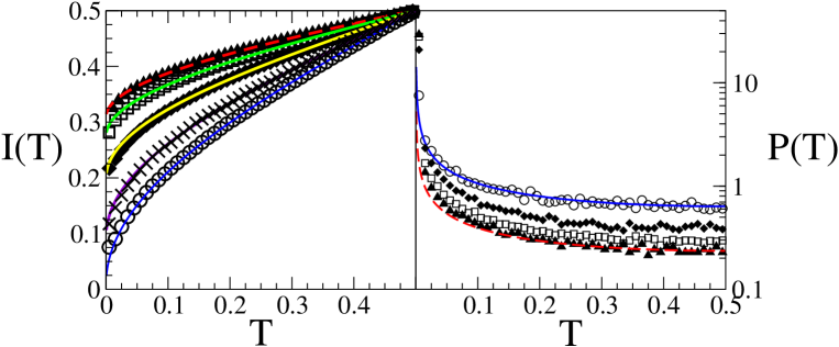
Figure 2: Left panel: Integrated probability distribution $I(T)$ of transmission eigenvalues for open kicked rotators with $\tau_{\rm D}/\tau_{\rm B}=25$ and $\tau_{\rm E}^{(2)}\simeq 0$ (empty circles; distribution calculated over 729 different samples); $\tau_{\rm D}/\tau_{\rm B}=5$, and $\tau_{\rm E}^{(2)}/\tau_{\rm B}=0.16$ ($\times$; 1681 samples), $\tau_{\rm E}^{(2)}/\tau_{\rm B}=1.5$ (black diamonds; 729 samples), $\tau_{\rm E}^{(2)}/\tau_{\rm B}=2.8$ (empty squares; 16 samples), and $\tau_{\rm E}^{(2)}/\tau_{\rm B}=4.1$ (black triangles; 2 samples). The blue, violet, yellow, green and red lines give the distribution $I_{\alpha}$ of Eq. (7), with $\alpha\approx 0.98$, 0.81, 0.6, 0.45 and 0.385 respectively. Right panel: Probability distribution $P(T)$ of transmission eigenvalues for the same set of parameters as in the main panel (data for $\tau_{\rm D}/\tau_{\rm B}=5$ and $\tau_{\rm E}^{(2)}/\tau_{\rm B}=1.5$ have been removed for clarity). The blue solid line gives the universal distribution $P_{\rm RMT}$ of Eq. (5) while the red dashed line corresponds to Eq. (6), with $\alpha=0.39$. Note that $P(T)$ is symmetric around $T=0.5$.

The emergence of classical determinism in the semiclassical limit reflects the fact that short trajectories are able to carry a wave packet in one piece through the system, provided that the wave packet is localized over a sufficiently small volume (see Fig. 1). Equation (6) moreover suggests that the spectrum of transmission eigenvalues is the sum of two independent contributions, precisely what would happen if the total electronic fluid of the system would split into two coexisting phases, a classical and a quantal one [36]. This splitting leads to a two-phase fluid model. It has been surmised that the quantal phase can be modelled by RMT [37], which results in an effective random-matrix model with renormalized matrix dimension $\alpha N$. Since $\alpha N\propto N^{1-1/\lambda\tau_{\rm D}}\to\infty$ in the semiclassical limit (see the related discussion of the fractal Weyl law in section 4), effective RMT predicts that the universality of quantum interference such as weak localization and parametric conductance fluctuations is not affected by a finite Ehrenfest time. This model is supported by a semiclassical theory based on the two-fluid model [38]. On the other hand, a stochastic quasiclassical theory which models mode-mixing by isotropic residual diffraction predicts that quantum interference effects are suppressed for a finite Ehrenfest time [27, 39, 40, 41].

Numerical investigations on parametric conductance fluctuations [35, 40, 43] give support for the RMT universality of the quantal phase (see Sec. 3.2), and variants of the effective RMT model have been successfully utilized beyond transport applications (see Secs. 4, 5). On the other hand, while an earlier numerical investigation of the weak-localization correction [42] reported no clear dependence of the magnetoconductance $\delta G=G(B=0)-G(B=\infty)$ on the Ehrenfest time, very recent investigations [39, 40] find a suppression of $\delta G$ for an increasing Ehrenfest time. The observed suppression is in agreement with the prediction $\delta G\propto\exp[-\tau_{\rm E}^{(2)}/\tau_{\rm D}]$ of a modified quasiclassical theory [40] in which the suppression results from electrons with dwell time between $\tau_{\rm E}^{(2)}$ and $2\tau_{\rm E}^{(2)}$. However, the quasiclassical theory cannot explain why the parametric conductance fluctuations are not suppressed. It also does not yet deliver as many predictions beyond transport as the effective RMT (for quasiclassical predictions of the mesoscopic proximity effect, see Sec. 5).

At present, both effective RMT as well as the quasiclassical theory have to be considered as phenomenological models, as they involve uncontrolled approximations. Clearly, a microscopic theory for the quantal phase which establishes the extent of its universality is highly desirable. This poses a considerable theoretical challenge considering that even in the limit of a vanishing Ehrenfest time a microscopic foundation for RMT in ballistic systems is only slowly emerging [44]. In this section, we focus on the consequences of the emergence of deterministic transport modes for the shot noise and the conductance fluctuations, as most of these consequences are largely independent of the precise degree of universality among the non-deterministic transport modes.

3.1 Suppression of shot noise

Shot noise is the non-thermal component of the electronic current fluctuations [45]

$$P(\omega)=2\int_{-\infty}^{\infty}\langle\delta I(t)\delta I(0)\rangle\exp(i\omega t)\,dt,$$ (8)

where $\delta I(t)=I(t)-\bar{I}$ is the deviation of the current from the mean current $\bar{I}$, and $\langle\ldots\rangle$ denotes the expectation value. This noise arises because of stochastic uncertainties in the charge carrier dynamics, which can be caused by a random injection process, or may develop during the transport through the system. For completely uncorrelated charge carriers, the noise attains the Poissonian value $P_{0}=2e^{2}GV$. Deviations from this value are a valuable indicator of correlations between the charge carriers.

Phase coherence requires sufficiently low temperatures, at which Pauli blocking results in a regular injection and collection of the charge carriers from the bulk electrodes. The only source of shot noise is then the quantum uncertainty with which an electron is transmitted or reflected. This is expressed by the quantum probabilities $0\leq T_{n}\leq 1$. In terms of these probabilities, the zero-frequency component of the shot noise is given by [46]

$$P(\omega=0)=2G_{0}eV\sum T_{n}(1-T_{n}).$$ (9)

This is always smaller than the Poisson value,which can be attributed to the Pauli blocking.

In RMT, the universal value of shot noise in cavities with symmetric openings follows from Eq. (5), $P(\omega=0)=\frac{1}{4}P_{0}$ [12]. It was predicted by Agam et al. [47] that shot noise is further reduced below this value when the Ehrenfest time is finite,

$$P(\omega=0)=\frac{1}{4}P_{0}\exp(-\tau_{\rm E}/\tau_{\rm D}).$$ (10)

The RMT value has been observed by Oberholzer et al. in shot-noise measurements on lateral quantum dots [48]. The same group later observed that the shot noise is reduced below the universal RMT result when the system is opened up (which reduces $\tau_{\rm D}/\tau_{\rm B}$, not $\tau_{\rm H}/\tau_{\rm B}$) [49, 50].

Equation (9) certifies that classically deterministic transport channels with $T_{n}=0$ or $T_{n}=1$ do not contribute to the shot noise [51]. Ref. [47] is based on the quasiclassical theory [27] which models mode-mixing by residual diffraction, and equates the Ehrenfest time with the closed-system Ehrenfest time $\tau_{\rm E}^{(0)}$. The discussion of the formation of the deterministic transport channels suggests that this has to be replaced by the transport Ehrenfest time $\tau_{\rm E}^{(2)}$ [33]. Subsequent numerical investigations have tested this prediction for the open kicked rotator [30]. Results for various degrees of chaoticity (quantified by the Lyapunov exponent $\lambda$) and dwell times $\tau_{\rm D}$ are shown in Fig. 3. The shot noise is clearly suppressed below the RMT value as the semiclassical parameter $M$ is increased. The right panel shows a plot of $-\ln(4P/P_{0})$ as a function of $\ln N^{2}/M\sim\ln(\tau_{\rm H}\tau_{\rm B}/4\tau_{\rm D}^{2})$. The data is aligned along lines with slope $1/\lambda\tau_{\rm D}$. This confirms that the suppression of the shot noise is governed by $\tau_{\rm E}^{(2)}$, in agreement with the distribution (6) of transmission eigenvalues.

Figure 3: Left and middle panels: dependence of the shot noise on the semiclassical parameter $M\sim\tau_{\rm H}/\tau_{\rm B}$ for two different Lyapunov exponents $\lambda$ and three different dwell times $\tau_{\rm D}$ of the open kicked rotator (as indicated in the plots). The solid line is the prediction from RMT. The dashed lines are obtained from a semiclassical estimate of the number of deterministic transport channels [37]. Right panel: rescaled data in a double-logarithmic plot, together with lines of slope $1/\lambda\tau_{\rm D}$. Figures adapted from Ref. [30].

3.2 From universal to quasiclassical conductance fluctuations

Universal conductance fluctuations are arguably one of the most spectacular manifestations of quantum coherence in mesoscopic systems [52]. In metallic samples, the universality of the conductance fluctuations manifests itself in their magnitude, ${\rm rms}\,G=O(G_{0})$, independently on the sample’s shape and size, its average conductance or the exact configuration of the underlying impurity disorder. In ballistic chaotic systems, a similar behavior is observed, which is captured by RMT [12, 13, 14]. At the core of the universality lies the ergodic hypothesis that sample-to-sample fluctuations are equivalent to fluctuations induced by parametric variations (e.g. changing the Fermi energy or applying a magnetic field) within a given sample [52].

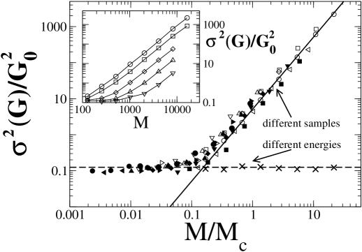
Figure 4: Variance $\sigma^{2}(G)$ of the conductance vs. the rescaled effective Hilbert space size $M/M_{c}$ in the open kicked rotator for parameters $K\in[9.65,27.65]$, $\tau_{\rm D}/\tau_{\rm B}\in[5,25]$, and $M\in[128,16384]$. The scaling parameter $M_{c}=2\pi(\tau_{\rm D}/\tau_{\rm B})^{2}\exp(\lambda\tau_{\rm B})$ varies by a factor $70$. The solid and dashed lines indicate the classical, sample-to-sample behavior $\propto M^{2}$, and the universal behavior $\sigma^{2}(G)=G_{0}^{2}/8$, respectively. Inset: unscaled data for $K=9.65$ and $\tau_{\rm D}/\tau_{\rm B}=5$ (circles), 7 (squares), 10 (diamonds), 15 (upward triangles) and 25 (downward triangles). Figure taken from Ref. [35].

Three numerical works explored the quantum-to-classical crossover of conductance fluctuations [35, 40, 43]. Their findings are consistent with each other and support the conclusion that (i) the ergodic hypothesis breaks down once $\tau_{\rm E}^{(2)}$ is no longer negligible; (ii) under variation of a quantum parameter such as the energy, the conductance fluctuations stay at their universal value, independently on $\tau_{\rm E}^{(2)}/\tau_{\rm D}$; and (iii) sample-to-sample fluctuations increase sharply above the universal value, $\sigma^{2}(G)\propto G_{0}^{2}(M/M_{c})^{2}$, when $M$ becomes larger than $M_{c}=2\pi(\tau_{\rm D}/\tau_{\rm B})^{2}\exp(\lambda\tau_{\rm B})$.

Findings (i)-(iii) are illustrated in Fig. 4, which presents results obtained from the open kicked rotator model. They can be understood on the basis of the two-phase dynamical fluid discussed above. The deterministic transport channels are insensitive to the variation of a quantum parameter that influences the phase accumulated on an unchanged classical trajectories. However, once one changes the sample configuration, all classical trajectories are scrambled and huge classical conductance fluctuations result. The size of the classical fluctuations is determined by the quantum mechanical resolution of classical phase space structures corresponding to the largest cluster of fully transmitted or reflected neighboring trajectories (see Ref. [37]), which yields the scaling with $M$ (inset of Fig. 4) and $M_{c}$ (main panel of Fig. 4). When a quantum parameter is varied, the conductance fluctuates only due to long, diffracting trajectories with $t>\tau_{\rm E}^{(2)}$, which build up the quantal phase. With the further assumption that the quantal phase is described by the effective RMT model, it follows that the parametric fluctuations are universal, independently on $\tau_{\rm E}^{(2)}$ (crosses in the main panel of Fig. 4). These conclusions are also supported by the observation in Ref. [35] that the energy conductance correlator $F(\varepsilon)=\sigma^{-2}(G)\;\langle\delta G(\varepsilon_{0})\delta G(\varepsilon_{0}+\varepsilon)\rangle$ decays on the universal scale of the Thouless energy, $\propto h/\tau_{\rm D}$, independently on $\tau_{\rm E}^{(2)}$.

4 Decay of quasi-bound states

Suppose that the particle is not injected by one of the openings but is instead prepared (e.g., as an excitation) inside the system and then escapes through the openings (we will consider the case of a single opening with $N_{\rm tot}\equiv N$ channels). Instead of the transport modes, this situation leads us to consider the decay modes of the system, determined by the stationary Schrödinger wave equation with outgoing boundary conditions. In contrast to the hermitian eigenvalue problem for a closed system, an open system with such boundary conditions features a non-selfadjoint Hamilton operator with complex energy eigenvalues and mutually non-orthogonal eigenmodes, called quasi-bound states [19, 21, 53]. The imaginary part of the complex energy $E=E^{\prime}-i\frac{\hbar\Gamma}{2}$ of a quasibound state is associated to its escape rate $\Gamma$ (hence, all eigenvalues lie in the lower half of the complex-energy plane). These energies coincide with the poles of the scattering matrix, which establishes a formal link between transport and escape. Since RMT encompasses also the energy dependence of the scattering matrix, it delivers precise predictions for the escape rates and wave functions of the quasi-bound states. Hence, we are again confronted with the issue to determine the range of applicability of these predictions in light of the signatures of classical determinism observed in the short-time dynamics up to the characteristic Ehrenfest time for the escape problem.

The universal RMT prediction for the escape rates can be obtained via two routes. The standard route relates the scattering matrix ${\cal S}$ to an effective $M\times M$-dimensional Hamiltonian matrix $H$ representing the closed billiard, and $M\times N$-dimensional matrices $W$ that couple it to the openings [19],

$${\cal S}(E)=1-2\pi iW^{T}(E-H+i\pi WW^{T})^{-1}W.$$ (11)

The superscript “$T$” indicates the transpose of the matrix. The poles of the scattering matrix are then obtained as the eigenvalues of the non-hermitian matrix $H-i\pi WW^{T}$. Assuming that $H$ is a random Gaussian matrix, one can obtain detailed predictions of the density of these eigenvalues for arbitrary coupling strength [21]. For $1\ll N\ll M$, the probability density of decay rates is then given by

$$P(\Gamma)=\frac{1}{\tau_{\rm D}\Gamma^{2}}\Theta(\Gamma-\tau_{\rm D}^{-1}),$$ (12)

where $\Theta$ is the unit step function.

The second route to the distribution of decay rates is particularly adaptable for the case of ballistic dynamics. It starts from the formulation of the scattering matrix in terms of an internal $M\times M$-dimensional scattering matrix $U(E)$, which describes the return amplitude to the confinement of the system [54, 55, 56]. For ballistic openings one has

$${\cal S}(E)=PU(E)[1-(1-P^{T}P)U(E)]^{-1}P^{T},$$ (13)

where $P\propto W$ such that $P^{T}P$ is an idempotent projector onto the leads. The poles of the scattering matrix are obtained as the solutions of the determinantal equation ${\rm det}\,[1-(1-P^{T}P)U(E)]=0$.

In the semiclassical limit $M\to\infty$, the matrix $U(E)$ carries an overall phase factor $\exp(i\nu(E))$ with phase velocity $d\nu/dE=\tau_{\rm B}/\hbar$, equivalent to a level spacing $\Delta=h/M\tau_{\rm B}=h/\tau_{\rm H}$. In RMT, the distribution of the poles is obtained under the assumption that $U(E)=F\exp(iE\tau_{\rm B}/\hbar)$ is proportional to a random unitary matrix $F$. The truncated unitary matrix $(1-P^{T}P)F$ has eigenvalues $\mu=\exp[-(iE^{\prime}/\hbar+\gamma/2)\tau_{\rm B}]$, where the decay constant $\gamma$ is related to the decay rate by $\Gamma=\frac{1}{\tau_{\rm B}}\left(1-e^{-\gamma\tau_{\rm B}}\right)$. The distribution of these decay constants is given by [57]

$$P(\gamma)=\frac{\tau_{\rm B}^{2}}{4\tau_{\rm D}\sinh^{2}(\gamma\tau_{\rm B}/2)}\Theta(1-e^{-\gamma\tau_{\rm B}}-\tau_{\rm B}/\tau_{\rm D}),$$ (14)

which is equivalent to Eq. (12).

RMT does not account for escape routes with a lifetime shorter than the Ehrenfest time. Recently, it has been found that these routes induce the formation of anomalously decaying quasi-bound states, with very large escape rate $\Gamma$ [34]. The semiclassical support of the associated wave functions is concentrated in a small area of phase space, (their total number is much larger than according to Weyl’s rule of one state per Planck cell). For illustration, Fig. 5 shows classical regions of escape after a few bounces in the open kicked rotator, along with two examples of anomalously decaying quasi-bound states, which are both localized in the same region of classical escape after one bounce. These states are contrasted with a slowly decaying state, which displays a random wave pattern.

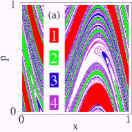
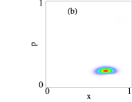
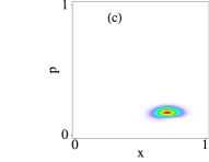
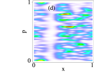
Figure 5: Panel (a): Classical regions of escape after one to four bounces (color code) in an open kicked rotator with $\tau_{\rm D}/\tau_{\rm B}=5$ and $K=7.5$ ($\lambda\tau_{\rm B}\approx 1.3$). Panels (b) and (c): Husimi representations of two anomalously decaying quasi-bound states for $M=160$. Panel (d): Husimi representations of a slowly-decaying quasi-bound state. Figure adapted from Ref. [34].

In order to discuss these observations, let us assume that the particle is initially represented by a localized wave packet $\chi_{0}$ (such as sketched in Fig. 1). The evolution of this wave packet from bounce to bounce with the confinement is given by

$$\chi_{m}=[(1-P^{T}P)U(E)]^{m}\chi_{0}.$$ (15)

When the final wave packet fits well through the opening the decay is sudden, hence not exponential at all. For such sudden escape the wave packets generated by the dynamical evolution all are associated to rather special eigenstates of the truncated operator $(1-P^{T}P)U(E)$: If the escape occurs after $n$ bounces, then

$$[(1-P^{T}P)U(E)]^{n-m}\chi_{m}=0$$ (16)

(neglecting the exponentially suppressed leakage out of the opening area). This corresponds to a highly degenerate eigenvalue $\mu=0$, hence, $\Gamma=\infty$.

Obviously, the (algebraic) multiplicity of this eigenvalue is at least $m$. However, in the semiclassical construction there is only one true eigenstate associated to this eigenvalue, namely, $\chi_{n-1}$. This deficiency is a consequence of the non-normality of the truncated unitary operator, for which the existence of a complete set of eigenvectors is not guaranteed. The degeneracy of the states is lifted beyond the semiclassical approximation, due to leakage out of the opening area. Hence, in practice one finds a complete set of eigenstates associated to this escape route, but the states are almost identical and hence are all supported by the same area in phase space.

As a consequence of the strong overlap of the anomalously decaying states, Weyl’s rule of covering the support of the states by Planck cells (of size $\sim 1/M$) cannot be used to estimate their number. The $m$ states $\chi_{n}$, however, are semiclassically orthogonal, and Eqs. (15) and (16) imply that they span the same eigenspace as the nearly degenerate eigenstates (they provide a Schur decomposition). The orthogonality of these states reinstates the applicability of Weyl’s rule. When we further observe that the semiclassical construction requires a reliable quantum-to-classical correspondence of the wave packet dynamics ($m\tau_{\rm B}<\tau_{\rm E}^{(1)}$), one can estimate the relative fraction $f$ of ballistically decaying states by the probability to escape faster than $\tau_{\rm E}^{(1)}$. Under the assumption of well developed classical ergodicity ($\tau_{\rm D}\gg\tau_{\rm B},\lambda^{-1}$), this probability is given by

$$f=1-\exp(-\tau^{(1)}_{\rm E}/\tau_{\rm D}),$$ (17)

with the escape Ehrenfest time given in Eq. (1) [34].

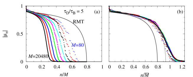
Figure 6: Ordered decay factors $|\mu_{n}|=\exp(-\gamma_{n}\tau_{B}/2)$ for an open kicked rotator with $\tau_{\rm D}/\tau_{\rm B}=5$ and $K=7.5$ ($\lambda\tau_{\rm B}\approx 1.3$) as a function of the relative indices $n/M$ [panel (a)] and $n/\overline{M}$ [panel (b)], for $M=2^{m}\times 80$, $m=0,1,2,\ldots,8$. The solid line in panel (a) is the RMT result of Eq. (18) with $\overline{M}=M$. The solid line in panel (b) is the same result with $\overline{M}$ given by Eq. (19–20). For the dashed line, this effective dimension has been fitted to the data. Figure adapted from Ref. [34].

Equation (17) has been tested numerically in the open kicked rotator by sorting all decay factors $|\mu_{n}|=\exp(-\gamma_{n}\tau_{\rm B}/2)$, $n=1,2,3,\ldots,M$, according to their magnitude (see Fig. 6). The data approximately collapses onto a single curve when the relative index $n/M$ is rescaled with $\exp(-\tau^{(1)}_{\rm E}/\tau_{\rm D})$. For small decay rates, the scaling function follows closely the RMT curve [57]

$$n(|\mu|)=\overline{M}[1-\frac{\tau_{\rm B}}{\tau_{\rm D}}(1-|\mu|^{2})^{-1}]\quad(|\mu|^{2}>1-\tau_{\rm B}/\tau_{\rm D}),$$ (18)

where the matrix dimension is rescaled to

$$\overline{M}=M\exp(-\tau^{(1)}_{\rm E}/\tau_{\rm D}).$$ (19)

This equation can be rewritten as

$$\overline{M}=M^{1-1/\lambda\tau_{\rm D}}(\tau_{\rm D}/\tau_{\rm B})^{1/\lambda\tau_{\rm D}},$$ (20)

which is precisely of the form of a fractal Weyl law [58, 59]. More generally, the exponent of $M$ in this law is related to the fractal dimension of the repeller in the system. Equation (20) applies under the conventional conditions for RMT universality ($\tau_{\rm B},\lambda^{-1}\ll\tau_{\rm D}\ll\tau_{\rm H}$), for which the low fractal dimensions can be approximated by $d=1-1/\lambda\tau_{\rm D}+O((\lambda\tau_{\rm D})^{-2})$ [60]. For a discussion of $d$ and the scaling function outside this universal regime see the article of Nonnenmacher and Zworski in the present issue [59].

5 Quantum-to-classical crossover in the mesoscopic proximity effect

We finally consider the situation of a ballistic metallic cavity in contact with a conventional superconductor, a so-called Andreev billiard [61, 62]. Compared to the normal billiards considered so far, the presence of superconductivity induces a new dynamical process called Andreev reflection, that is, retroreflection accompanied by electron-hole conversion [63]. This process prevents individual low-energy quasiparticles from entering the superconductor.

For chaotic billiards it has been found that an excitation gap is formed as a consequence of the Andreev reflection, in that the Density of States (DoS) in the cavity is suppressed at the Fermi level. The energetic scale of this gap is the ballistic Thouless energy $E_{\rm T}=\hbar/2\tau_{\rm D}$, where $\tau_{\rm D}$ is the average time between two consecutive Andreev reflections [22]. For simplicity we consider the case of a single superconducting terminal with $N_{\rm tot}\equiv N$ open channels at the Fermi energy.

5.1 Bohr-Sommerfeld quantization versus random-matrix theory

In an ergodic cavity, all classical trajectories except a set of zero measure eventually collide with the superconducting interface. Andreev retroreflection is perfect at the Fermi energy, where the hole exactly retraces the electronic path. For a nonzero electronic excitation energy $E>0$, electron-hole symmetry is broken, and consequently there is a mismatch between the incidence and the retroreflection angle. For the lowest excitation energies $\propto E_{\rm T}$ in the limit $\lambda\tau_{\rm D}\gg 1$, this mismatch is a small parameter. Consequently, all electron-hole trajectories become periodic. In the semiclassical limit where both the perimeter $L$ of the cavity and the width $W$ of the contact to the superconductor are much larger than $\lambda_{\rm F}$ (hence $M,N\gg 1$), the semiclassical Bohr-Sommerfeld quantization rule relates the mean DoS to the return probability $P(t)$ to the superconductor [22],

$$\rho(E)=N\int_{0}^{\infty}{\rm d}tP(t)\sum_{m=0}^{\infty}\delta\left[E-(m+\frac{1}{2})\frac{\pi\hbar}{t}\right].$$ (21)

The shift by $1/2$ inside the $\delta$-function is due to two consecutive phase shifts of $\pi/2$ at each Andreev reflection. This ensures that no contributions with an energy smaller than $E_{\rm min}(t)=\pi\hbar/2t$ emerge from trajectories of duration $t$. Since a chaotic cavity has an exponential distribution of return times $P(t)\propto\exp[-t/\tau_{\rm D}]$ [64], Eq. (21) predicts an exponential suppression of the DoS in the chaotic case [65],

$$\rho(E)=\frac{N\tau_{\rm D}}{\pi}\frac{(2\pi/E\tau_{\rm D})^{2}\cosh(2\pi/E\tau_{\rm D})}{\sinh^{2}(2\pi/E\tau_{\rm D})}.$$ (22)

The DoS can also be calculated in the framework of RMT. The excitation spectrum is obtained in the scattering approach from the determinantal quantization condition [14]

$${\rm Det}[1+{\cal S}(E){\cal S}^{*}(-E)]=0.$$ (23)

By Eq. (11), the scattering matrix ${\cal S}$ is then related to a Hamiltonian matrix $H$. For low energies, Eq. (23) can be transformed into an eigenvalue equation for an effective Hamiltonian [66]

$${\rm Det}[E-H_{\rm eff}]=0\;\;,\;\;\;\;\;\;H_{\rm eff}=\left(\begin{array}[]{cc}H&-\pi PP^{T}\\ -\pi PP^{T}&-H^{*}\end{array}\right).$$ (26)

Assuming that $H$ is a random matrix, it has been found that the excitation spectrum exhibits a hard gap with a ground-state energy $E_{\rm RMT}\approx 0.6\,E_{\rm T}$ [22]. At first glance, both the Bohr-Sommerfeld and the RMT approach are expected to apply for chaotic cavities with $\lambda^{-1}$, $\tau_{\rm B}\ll\tau_{\rm D}$. The hard gap prediction of RMT has thus to be reconciled with the exponential suppression (22) from Bohr-Sommerfeld quantization.

A path toward the solution to this gap problem was suggested by Lodder and Nazarov [67], who argued that the Bohr-Sommerfeld quantization is valid only for return times smaller than the relevant Ehrenfest time, which was later identified with $\tau_{\rm E}^{(2)}$ [given in Eq. (1)] [33]. For $\tau_{\rm E}^{(2)}/\tau_{\rm D}\gg 1$, it was predicted that the hard RMT gap opens up at an energy $\simeq\hbar/\tau_{\rm E}^{(2)}$ in the Bohr-Sommerfeld DoS. A mechanism for the opening of this gap was soon proposed by Adagideli and Beenakker [68]. Constructing a perturbation theory, they showed that diffraction effects at the contact with the superconductor become singular in the semiclassical limit, which results in the opening of a gap at the inverse Ehrenfest time. More recent analytical and numerical works confirm that the solution to the gap problem lies in the competition between the Ehrenfest time and dwell time scales [29, 33, 69, 70, 71, 73, 74].

5.2 Ehrenfest suppression of the gap

At present there are two theories for quantizing Andreev billiards in the deep semiclassical limit. The first one proceeds along the lines of the two-phase fluid model and the effective RMT discussed in Section 3, but extended to take the energy dependence of the scattering matrix into account [70, 73]. The system’s scattering matrix is decomposed into two parts,

$$S_{0}(E)=S_{\rm cl}(E)\oplus S_{\rm qm}(E),$$ (27)

where the classical part $S_{\rm cl}(E)$ of dimension $M(1-\exp[-\tau_{\rm E}^{(2)}/\tau_{\rm D}])$ is complemented by a quantal part $S_{\rm eff}(E)$ of dimension $M\exp[-\tau_{\rm E}^{(2)}/\tau_{\rm D}]$. The excitation spectrum hence splits into classical contributions originating from scattering trajectories shorter than the Ehrenfest time, and quantum contributions supported by longer trajectories for which diffraction effects are important. An adiabatic quantization procedure allows to extract the classical part of the excitation spectrum, while diffraction effects are included in the theory via effective RMT, $S_{\rm qm}(E)=\exp[iE\tau_{\rm E}^{(2)}/\hbar]S_{\rm RMT}$, where $S_{\rm RMT}$ is a random matrix from the appropriate circular ensemble, while the factor $\exp[iE\tau_{\rm E}^{(2)}/\hbar]$ accounts for the delayed onset of random interference.

The second theory, due to Vavilov and Larkin [33], is based on the quasiclassical theory of Ref. [27], which models the mode mixing in the long time limit by isotropic residual diffraction, with the diffraction time set to $\tau_{\rm E}^{(2)}$. Standard techniques based on ensemble averaging can then be applied. In the limit $\tau_{\rm E}^{(2)}\ll\tau_{\rm D}$,the predictions of both theories for the gap value (given by the smallest excitation energy $\epsilon_{0}$) differ by a factor of $2$ [62],

$$\frac{\epsilon_{0}}{E_{\rm RMT}}=1-\frac{\alpha\tau_{\rm E}^{(2)}}{2\tau_{\rm D}},\;\;\;\;\alpha=\left\{\begin{array}[]{cc}2\sqrt{5}-4&{\rm effective\;RMT},\\ \sqrt{5}-2&{\rm quasiclassical\;theory}.\end{array}\right.$$ (28)

In the other limit $\tau_{\rm E}^{(2)}\gg\tau_{\rm D}$, both theories predict $\epsilon_{0}=\pi\hbar/2\tau_{\rm E}^{(2)}$ [62]. In the transient region $\tau_{\rm E}^{(2)}\simeq\tau_{\rm D}$, the two theories are parametrically different. These discrepancies have motivated detailed numerical investigations (based on the Andreev kicked rotator described in the Appendix) which we now review [29, 71, 73].

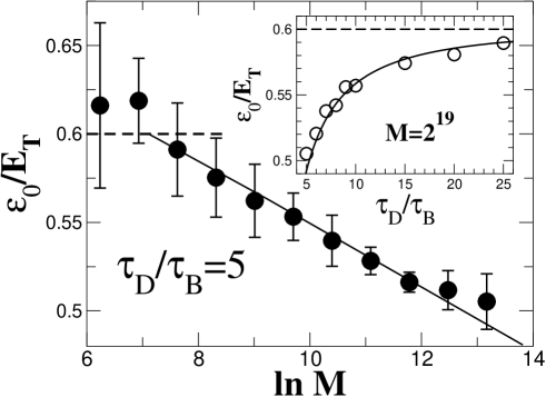
Figure 7: Main plot: Dependence of the mean Andreev gap on the system size $M$, for open kicked rotators with $\tau_{\rm D}/\tau_{\rm B}=5$ and $K=14$. Averages have been calculated with 400 (for $M=512$) to 40 (for $M>5\cdot 10^{5}$) different positions of the contacts to the superconductor. The error bars represent the root-mean-square of $\epsilon_{0}$. The dashed line is the RMT prediction and the solid line is a linear fit to the data points. Inset: Dependence of the mean gap on $\tau_{\rm D}/\tau_{\rm B}$ for $K=14$ and $M=524288$. The dashed line is the RMT prediction and the solid curve is given by Eq. (28), with coefficients extracted from the linear fit in the main plot. Figure adapted from Ref. [29].

We first show in Fig. 7 the systematic reduction of the excitation gap observed upon increasing the ratio $\tau_{\rm E}^{(2)}/\tau_{\rm D}$. The data corresponds to fixed classical configurations (dwell time and Lyapunov exponent) with variation of the semiclassical parameter $M$. The main panel is a semi-logarithmic plot of $\epsilon_{0}/E_{\rm T}$ as a function of $M\in[2^{9},2^{19}]$, for $\tau_{\rm D}/\tau_{\rm B}=5$ and $K=14$, well in the fully chaotic regime ($\lambda\tau_{\rm B}\approx 1.95$). The data has been fitted to

$$\frac{\epsilon_{0}}{E_{\rm RMT}}=1-\frac{\alpha}{2\lambda\tau_{\rm D}}\left[\ln(N^{2}/M)-\alpha^{\prime}\right],$$ (29)

as implied by Eq. (28) (the parameter $\alpha^{\prime}$ accounts for model-dependent subleading corrections to the Ehrenfest time). We find $\alpha=0.59$ and $\alpha^{\prime}=3.95$. Once $\alpha$ and $\alpha^{\prime}$ are extracted, one obtains a parameter-free prediction for the dependence of the gap on $\tau_{\rm D}/\tau_{\rm B}$, which is shown as the solid line in the inset to Fig. 7. We conclude that Eq. (28) gives the correct parametric dependence of the Andreev gap for small Ehrenfest times. Within the numerical uncertainties, the value of $\alpha$ conforms with the prediction of effective RMT. Similar conclusions were drawn in Ref. [74] from numerical investigations of Sinai billiards.

5.3 Quasiclassical fluctuations of the gap

The distribution $P(\epsilon_{0})$ of the Andreev gap has been calculated within RMT in Ref. [75]. It was shown to be a universal function of the rescaled parameter $(\epsilon_{0}-E_{\rm RMT})/\Delta_{N}$, where $\Delta_{N}=0.068N^{1/3}\Delta$ gives the mean level spacing right above the gap in terms of the bulk level spacing $\Delta$. Similarly, the standard deviation of the distribution is given by $\sigma(\epsilon_{0})=1.27\Delta_{N}$.

The universality of the gap distribution is violated when the Ehrenfest time is finite. As in the case of the conductance, the sample-to-sample gap fluctuations are then dominated by classical fluctuations. In a simple approximation, the effective RMT model gives a qualitative prediction for the gap value in the crossover from a small to a large Ehrenfest time [70],

$$\epsilon_{0}=\frac{E_{\rm RMT}}{1+\tau_{\rm E}^{(2)}/\tau_{\rm D}}.$$ (30)

A more precise form of the gap function was derived in Ref. [62]. Sample-to-sample fluctuations can be incorporated into the effective RMT model when one replaces the dwell time in Eq. (30) by the mean dwell time of long trajectories, that is one makes the substitution

$$(\tau_{\rm E}^{(2)}+\tau_{\rm D})\rightarrow\langle t\rangle_{*}=\int_{\tau_{\rm E}^{(2)}}^{\infty}{\rm d}t\,tP(t)\;\Bigg{/}\;\int_{\tau_{\rm E}^{(2)}}^{\infty}{\rm d}t\,P(t).$$ (31)

This was done in Ref. [71]. The result with the correct gap function from Ref. [62] is shown in Fig. 8 [72]. It is seen that the gap fluctuations are greatly enhanced to the same order of magnitude as the gap itself. It was indeed found that $\sigma(\epsilon_{0})$ becomes a function of $\tau_{\rm D}$ only in the limit of large $M$. From Fig. 8, correlations between sample-to-sample variations of $\epsilon_{0}$ and $\langle t\rangle_{*}^{-1}$ are evident, clearly establishing the classical origin of the sample-to-sample fluctuations in the large $M$ regime.

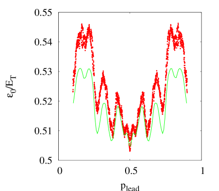
Figure 8: Quantum mechanical gap values $\epsilon_{0}$ of the Andreev kicked rotator as a function of the position $p_{\rm{lead}}$ of the center of the interface with the superconductor, for parameter values $M=131072$, $\tau_{\rm D}/\tau_{\rm B}=5$, $K=14$. The solid line uses effective RMT to relate the gap fluctuations to the fluctuations of the mean dwell time $\langle t\rangle_{*}$ of long classical trajectories, defined in Eq. (31). Figure courtesy of Marlies Goorden [72].

Together with the average value and sample-to-sample fluctuations of $\epsilon_{0}$, additional numerical evidence for the validity of the two-phase fluid model in Andreev billiards was presented in Refs. [71, 73]. Most notably, the critical magnetic field at which the gap closes was found to be determined by the competition between two values, $B_{c}^{\rm{eff}}$ and $B_{c}^{\rm{ad}}$. These fields correspond, respectively, to the disappearance of the gap for the quantum, effective RMT part and the classical, adiabatically quantized part of the spectrum. Moreover, Ref. [73] showed how most of the full density of states at finite $\tau_{\rm E}^{(2)}/\tau_{\rm D}$ can be obtained from the effective RMT model. It would be desirable to have similar predictions from the quasiclassical theory that could be checked against numerical data. The excellent agreement between the numerical data and the predictions from the effective RMT model in Andreev billiards only adds to the intriguing controversy about the universality of the quantal phase in the two-fluid model, which we encountered at various places in this review.

6 Summary and conclusions

We gave an overview over recent theoretical and numerical investigations which address the emergence of quantum-to-classical correspondence in mesoscopic systems with a finite Ehrenfest time. By now there is overwhelming evidence that the quasi-deterministic short-time dynamics up to the Ehrenfest time jeopardizes the universality otherwise exhibited by quantized open chaotic systems. This was illustrated in the discussion of three different physical situations: transport, decay of quasi-bound states, and the mesoscopic proximity effect.

While there is consensus over the role of deterministic transport and decay modes, there are two competing theoretical frameworks with different predictions for the degree of wave chaos in the long-time dynamics beyond the Ehrenfest time, namely, the effective random-matrix theory [37] and the stochastic quasiclassical theory [27]. Both theories incorporate the deterministic short-time wave-packet dynamics in similar ways, and correctly explain the suppression of shot-noise power as well as the emergence of classical sample-to-sample fluctuations in the semiclassical limit. However, the two theories model the long-time dynamics in different ways, namely, via a random-matrix of reduced dimension or via residual diffraction. Consequently, the effective RMT predicts that quantum interference corrections like the weak-localization correction and parametric conductance fluctuations stay universal deep in the semiclassical limit, while the quasi-classical theory predicts a suppression of these effects in this limit. Moreover, there is conflicting numerical evidence for these coherent effects, with all the indications that more surprises are likely to be uncovered. In view of this intriguing situation, more theoretical and numerical efforts to uncover the limits of universality in mesoscopic systems, while challenging, are clearly desirable.

7 Acknowledgements

We thank İ. Adagideli, C. Beenakker, P. Brouwer, M. Goorden, E. Sukhorukhov, A. Tajic, J. Tworzydło and R. Whitney for fruitful collaborations on projects related to the topics discussed here. C. Beenakker and P. Brouwer provided useful comments on several important points. M. Goorden kindly provided us with Fig. 8 from her PhD thesis [72]. This work has been supported by the Swiss National Science Foundation and the Max Planck Institute for the Physics of Complex Systems, Dresden.

Appendix: open kicked rotators

The logarithmic increase of the Ehrenfest time with the effectuve Hilbert space size $M$ requires an exponential increase in the latter to investigate the ergodic semiclassical regime $\tau_{\rm E}\gtrsim\tau_{\rm D}$, $\lambda\tau_{\rm D}\gg 1$, in which deviations from RMT universality emerge due to quantum-to-classical correspondence. The numerical results reviewed in this paper are all obtained for a particular class of systems, the open kicked rotator [29, 30, 31, 32], for which very efficient methods based on the fast-Fourier transform exist. Combined with the Lanczos exact diagonalization algorithm, as first suggested in Ref. [76], these methods allowed to reach system size in excess of $M=10^{6}$ for the Andreev billiard problem [29].

The classical dynamics of the closed system are given by a symmetrized version of the standard map on the torus $x,p\in[0,2\pi]$ [4],

$$\left\{\begin{array}[]{lll}\bar{x}&=&x+p+\frac{K}{2}\sin x\quad(\,{\rm mod}\,2\pi)\\ \bar{p}&=&p+\frac{K}{2}(\sin x+\sin\bar{x})\quad(\,{\rm mod}\,2\pi).\end{array}\right.$$ (34)

Each iteration of the map (34) corresponds to one scattering time $\tau_{\rm B}$ off the boundaries of a fictitious cavity. The dynamics of this system ranges from fully integrable ($K=0$) to well-developed chaos [$K\geq 7$, with Lyapunov exponent $\lambda\approx\tau_{\rm B}^{-1}\ln(K/2)$].

The map (34) can be quantized by discretization of the space coordinates $x_{m}=2\pi m/M$, $m=1,\ldots M$. The quantum representation is then provided by a unitary $M\times M$ Floquet operator $F$ [8], which gives the time evolution for one iteration of the map. For our specific choice of the kicked rotator, the Floquet operator has matrix elements

$$F_{m,m^{\prime}} = M^{-1/2}\exp\{-(iMK/4\pi)[\cos(2\pi m/M)+\cos(2\pi m^{\prime}/M)]\}$$ (35)

$$\times\sum_{l}\exp[2\pi il(m-m^{\prime})/M]\exp[-(\pi i/2M)l^{2}].$$

The spectrum $\exp(-iE_{n}\tau_{B}/\hbar)$ of $F$ defines a discrete set of $M$ quasienergies $E_{n}\in[0,h/\tau_{B})$ with an average level spacing $\Delta=h/M\tau_{B}$.

For the transport problem, the system is opened up by defining two ballistic openings via absorbing phase space strips $[x_{L}-\delta x,x_{L}+\delta x]$ and $[x_{R}-\delta x,x_{R}+\delta x]$, each of a width $2\delta x=\pi\tau_{\rm B}/\tau_{\rm D}$. Much in the same way as in the Hamiltonian case [19], a quasienergy-dependent $2N\times 2N$ scattering matrix can be determined from the Floquet operator $F$ as [56]

$${\cal S}(E)=P[\exp(-iE\tau_{B}/\hbar)-F(1-P^{T}P)]^{-1}FP^{T}.$$ (36)

The $2N\times M$-dimensional matrix $P$ describes the coupling to the leads, and is given by

$$P_{n,m}=\left\{\begin{array}[]{ll}1&\mbox{if $n=m\in\{(x_{\rm R,L}-\delta)M/2\pi,x_{\rm R,L}+\delta)M/2\pi\}$}\\ 0&\mbox{otherwise.}\end{array}\right.$$ (39)

The number of channels in each opening is given by $N=\,{\rm Int}\,[\delta M/\pi]$. An ensemble of samples with the same microscopic properties can be defined by varying the position of the two openings for fixed $\tau_{\rm D}/\tau_{\rm B}$ and $K$, or by varying the energy $E$.

For the escape problem, $P$ couples only to a single opening, and the quasibound states are obtained by diagonalization of the truncated quantum map $(1-P^{T}P)F$.

So far we described particle excitations in a normal metal. In order to model an Andreev billiard [29], we also need hole excitations. A particle excitation with energy $E_{m}$ (measured relatively to the Fermi level) is identical to a hole excitation with energy $-E_{m}$ which propagates backwards in time. This means that hole excitations in a normal metal have Floquet operator $F^{\ast}$. Andreev reflections occurs at the opening to the superconducting reservoir, which is again represented by the matrix $P$. The symmetrized quantum Andreev map is finally constructed from the matrix product

$${\cal F}={\cal P}^{1/2}\left(\begin{array}[]{cc}F&0\\ 0&F^{\ast}\end{array}\right){\cal P}^{1/2},\;\;{\cal P}=\left(\begin{array}[]{cc}1-P^{\rm T}P&-iP^{\rm T}P\\ -iP^{\rm T}P&1-P^{\rm T}P\end{array}\right).$$ (44)

The excitation spectrum is obtained by diagonalization of ${\cal F}$, whose quasienergy spectrum exhibits two gaps at $E=0$ and $E=h/2\tau_{\rm B}$. It can be shown that the excitation spectrum is identical to the solutions of the conventional determinantal equation ${\rm det}\,[1+{\cal S}(E){\cal S}^{*}(E)]=0$, where the scattering matrix is given by Eq. (36).

References

- [1] L.P. Kouwenhoven, C.M. Marcus, P.L. McEuen, S. Tarucha, R.M. Westervelt, and N.S. Wingreen, in Electron Transport in Quantum Dots, Nato ASI conference proceedings, Eds.: L.P. Kouwenhoven, G. Schön, and L.L. Sohn (Kluwer, Dordrecht, 1997)
- [2] Y. Alhassid, Rev. Mod. Phys. 72, 895 (2000).
- [3] I.L. Aleiner, P.W. Brouwer, and L.I. Glazman, Phys. Rep. 358, 309 (2002).
- [4] A.J. Lichtenberg and M.A. Lieberman, Regular and Chaotic Dynamics, Applied Mathematical Sciences Vol 38 (Springer, New York, 1992).
- [5] E. Ott, Chaos in Dynamical Systems (Cambridge University Press, Cambridge, 1993).
- [6] H.U. Baranger, R.A. Jalabert, and A.D. Stone, Phys. Rev. Lett. 70, 3876 (1993); Chaos 3, 665 (1993).
- [7] C.M. Marcus, R.M. Westervelt, P.F. Hopkings, and A.C. Gossard, Chaos 3, 643 (1993).
- [8] F. Haake, Quantum Signatures of Chaos, 2nd ed. (Springer, Berlin, 2001).
- [9] H.-J. Stöckmann, Quantum Chaos, (Cambridge University Press, Cambridge, 1999).
- [10] O. Bohigas, M.-J. Giannoni, and C. Schmit, Phys. Rev. Lett. 52, 1 (1984).
- [11] M.V. Berry, Proc. R. Soc. London A 400, 229 (1985).
- [12] R.A. Jalabert, J.-L. Pichard, and C.W.J. Beenakker, Europhys. Lett. 27, 255 (1994).
- [13] H.U. Baranger and P.A. Mello, Phys. Rev. Lett. 73, 142 (1994).
- [14] C.W.J. Beenakker, Rev. Mod. Phys. 69, 731 (1997).
- [15] R. Landauer, Phil. Mag. 21, 863 (1970).
- [16] M. Büttiker, Phys. Rev. Lett. 57, 1761 (1986).
- [17] R. Blümel and U. Smilansky, Phys Rev. Lett. 64, 241 (1990).
- [18] M. L. Mehta, Random Matrices (Acadamic Press, New York, 1991).
- [19] T. Guhr, A. Müller-Groeling, and H.A. Weidenmüller, Phys. Rep. 299, 189 (1998).
- [20] K. B. Efetov, Supersymmetry in Disorder and Chaos (Cambridge University Press, Cambridge, 1997).
- [21] Y.V. Fyodorov and H.-S. Sommers, J. Math. Phys. 38, 1918 (1997).
- [22] J.A. Melsen, P.W. Brouwer, K.M. Frahm, and C.W.J. Beenakker, Europhys. Lett. 35, 7 (1996); Physica Scripta T69, 223 (1997).
- [23] K.B. Efetov, Adv. Phys. 32, 53 (1983).
- [24] P.W. Brouwer, Phys. Rev. B 51, 16878 (1995).
- [25] R. G. Nazmitdinov, K. N. Pichugin, I. Rotter, and P. eba, Phys. Rev. E 64, 056214 (2001); Phys. Rev. B 66, 085322 (2002); R.G. Nazmitdinov, H.-S. Sim, H. Schomerus, and I. Rotter, Phys. Rev. B 66, 241302(R)(2002).
- [26] C.H. Lewenkopf and H.A. Weidenmüller, Ann. Phys. (N.Y.) 212, 53 (1991).
- [27] I.L. Aleiner and A.I. Larkin, Phys. Rev. B 54, 14423 (1996).
- [28] G.P. Berman and G.M. Zaslavsky, Physica A 91, 450 (1978).
- [29] Ph. Jacquod, H. Schomerus, and C.W.J. Beenakker, Phys. Rev. Lett. 90, 116801 (2003).
- [30] J. Tworzydlo, A. Tajic, H. Schomerus, and C.W.J. Beenakker, Phys. Rev. B 68, 115313 (2003).
- [31] F. Borgonovi, I. Guarneri, and D. L. Shepelyansky, Phys. Rev. A 43, 4517 (1991); F. Borgonovi and I. Guarneri, J. Phys. A 25, 3239 (1992).
- [32] A. Ossipov, T. Kottos, and T. Geisel, Europhys. Lett. 62 , 719 (2003).
- [33] M.G. Vavilov and A.I. Larkin, Phys. Rev. B 67, 115335 (2003).
- [34] H. Schomerus and J. Tworzydlo, Phys. Rev. Lett. 93, 154102 (2004).
- [35] Ph. Jacquod and E.V. Sukhorukov, Phys. Rev Lett. 92 116801 (2004).
- [36] A RMT distribution of transmission eigenvalues is also obtained in regular cavities with sufficient diffraction at the openings, see: F. Aigner, S. Rotter, and J. Burgdörfer, Phys. Rev. Lett. 94, 216801 (2005); P. Marconcini, M. Macucci, G. Iannaccone, B. Pellegrini, and G. Marola, cond-mat/0411691. Eq. (6) thus does not prove that the classical system is chaotic.
- [37] P.G. Silvestrov, M.C. Goorden, and C.W.J. Beenakker, Phys. Rev. B 67, 241301(R) (2003).
- [38] R.S. Whitney and Ph. Jacquod, Phys. Rev. Lett. 94, 116801 (2005).
- [39] S. Rahav and P.W. Brouwer, cond-mat/0505250.
- [40] S. Rahav and P.W. Brouwer, cond-mat/0507035.
- [41] I. Adagideli, Phys. Rev. B 68, 233308 (2003).
- [42] J. Tworzydlo, A. Tajic and C.W.J. Beenakker, Phys. Rev. B 70, 205324 (2004).
- [43] J. Tworzydlo, A. Tajic and C.W.J. Beenakker, Phys. Rev. B 69, 165318 (2003).
- [44] K. Richter and M. Sieber, Phys. Rev. Lett. 89, 206801 (2002); S. Müller et al., Phys. Rev. Lett. 93, 014103 (2004).
- [45] For a review on shot noise, see: Ya.M. Blanter and M. Büttiker, Phys. Rep. 336, 1 (2000).
- [46] M. Büttiker, Phys. Rev. Lett. 65, 2901 (1990).
- [47] O. Agam, I. Aleiner, and A. Larkin, Phys. Rev. Lett. 85, 3153 (2000).
- [48] S. Oberholzer, E. V. Sukhorukov, C. Strunk, C. Schönenberger, T. Heinzel, and M. Holland, Phys. Rev. Lett. 86, 2114(2001).
- [49] S. Oberholzer, E.V. Sukhorukov, and C. Schönenberger, Nature (London) 415, 765 (2002).
- [50] C. W. J. Beenakker and C. Schönenberger, Physics Today 85, No. 5, 37 (May 2003).
- [51] C.W.J. Beenakker and H. van Houten, Phys. Rev. B 43, 12066 (1991).
- [52] B.L. Altshuler, JETP Letters 41, 648 (1985); P.A. Lee and A.D. Stone, Phys. Rev. Lett. 55, 1622 (1985).
- [53] E.E. Narimanov, G. Hackenbroich, Ph. Jacquod, and A.D. Stone, Phys. Rev. Lett. 83, 4991 (1999).
- [54] B. Georgeot and R.E. Prange, Phys. Rev. Lett. 74, 4110 (1995); R.E. Prange, Phys. Rev. Lett. 90, 070401 (2003).
- [55] A.M. Ozorio de Almeida and R.O. Vallejos, Physica E 9, 488-493 (2001); R.O. Vallejos and A.M. Ozorio de Almeida, Ann. Phys. 278, 86-108 (1999).
- [56] Y.V. Fyodorov and H.-J. Sommers, JETP Letters 72, 422 (2000).
- [57] K. Życzkowski and H.-J. Sommers, J. Phys. A: Math. Gen. 33, 2045 (2000).
- [58] W. T. Lu, S. Sridhar, and M. Zworski, Phys. Rev. Lett. 91, 154101 (2003).
- [59] S. Nonnemacher and M. Zworski, present issue.
- [60] C. Beck and F. Schloegel, Thermodynamics of Chaotic Systems: An Introduction (Cambridge University Press, Cambridge, 1993).
- [61] I. Kosztin, D.L. Maslov, and P.M. Goldbart, Phys. Rev. Lett. 75, 1735 (1995).
- [62] For a recent review on Andreev billiards, see: C.W.J. Beenakker, Lect. Notes Phys. 667, 131 (2005); cond-mat/0406018.
- [63] A.F. Andreev, Sov. Phys. JETP 19, 1228 (1964).
- [64] W. Bauer and G.F. Bertsch, Phys. Rev. Lett. 65, 2213 (1990).
- [65] H. Schomerus and C.W.J. Beenakker, Phys. Rev. Lett. 82, 2951 (1999).
- [66] K.M. Frahm, P.W. Brouwer, J.A. Melsen, and C.W.J. Beenakker, Phys. Rev. Lett. 76, 2981 (1996).
- [67] A. Lodder and Yu.V. Nazarov, Phys. Rev. B 58, 5783 (1998).
- [68] İ. Adagideli and C.W.J. Beenakker, Phys. Rev. Lett. 89, 237002 (2002).
- [69] D. Taras-Semchuk and A. Altland, Phys. Rev. B 64, 014512 (2001).
- [70] P.G. Silvestrov, M.C. Goorden, and C.W.J. Beenakker, Phys. Rev. Lett. 90, 116801 (2003).
- [71] M.C. Goorden, Ph. Jacquod, and C.W.J. Beenakker, Phys. Rev. B 68, 220501 (2003).
- [72] M.C. Goorden, PhD thesis (Leiden, 2005).
- [73] M.C. Goorden, Ph. Jacquod, and C.W.J. Beenakker, cond-mat/0505206; to appear in Phys. Rev. B.
- [74] A. Kormanyos, Z. Kaufmann, C.J. Lambert, and J. Cserti, Phys. Rev. B 70, 052512 (2004).
- [75] M.G. Vavilov, P.W. Brouwer, V. Ambegaokar, and C.W.J. Beenakker, Phys. Rev. Lett. 86, 874 (2001).
- [76] R. Ketzmerick, K. Kruse, and T. Geisel, Physica D 131, 247 (1999).