Josephson current through a molecular transistor in a dissipative environment

Abstract

We study the Josephson coupling between two superconductors through a single correlated molecular level, including Coulomb interaction on the level and coupling to a bosonic environment. All calculations are done to the lowest, i.e., the fourth, order in the tunneling coupling and we find a suppression of the supercurrent due to the combined effect of the Coulomb interaction and the coupling to environmental degrees of freedom. Both analytic and numerical results are presented.

I Introduction

Mesoscopic systems connected to superconducting leads have been investigated for a number of years. If the mesoscopic system itself is superconducting the transport is influenced by the so-called parity effect in the Coulomb blockade regime.Averin and Nazarov (1992); Tuominen et al. (1992) For normal metal grains, the effect of the superconductivity is merely to modify the tunneling density of states due to the density of the superconducting leads, thus introducing an additional gap in the current-voltage characteristics.

Naturally, the Josephson current is also affected by the Coulomb correlations, because the transfer of a Cooper pair charges the mesoscopic system by two electron charges. This process is similar to a cotunneling event, and in the limit of large Coulomb repulsion, the path that involves double occupancy of the central region is not allowed, which results in a suppression of the Josephson coupling. This has been studied extensively in a number of theoretical works, starting with the work of Shiba and SodaShiba and Soda (1969) and Glazman and Matveev,Glazman and Matveev (1989) who calculated the Josephson current in the limit of infinite Coulomb repulsion and in perturbation theory, the leading order being the fourth order in the tunneling amplitudes. Interestingly, the Josephson current was shown to change its sign when the level which supports the tunneling current becomes occupied. This so-called $\pi$ junction behavior, which is consequently also relevant in the Kondo regime, has been studied in a number of papers.Spivak and Kivelson (1991); Ishizaka et al. (1995); Clerk and Ambegaokar (2000); Rozhkov et al. (2001); Vecino et al. (2003); Siano and Egger (2004); Zaikin (2004) For larger dots the interplay of the above mentioned parity effect and the Josephson effect has also been addressed.Bauernschmitt et al. (1994)

Experimentally, there has been a number of studies of metallic wires connected to superconductors,Scheer et al. (1997, 1998) but only a few studies in the Coulomb blockade regime. Buitelaar et al.Buitelaar et al. (2002, 2003) have observed multiple Andreev reflections and Kondo physics in carbon nanotube quantum dots. The supercurrent was not directly observed.

In this paper, we study the Josephson coupling through a single level system coupled to vibrational or dissipative environments. This is relevant for molecular transistor systems where strong influence of the coupling to various vibrational modes have been observed.Park et al. (2000); Yu and Natelson (2004); Yu et al. (2004) In the case of normal metal leads this has lead to a number of related theoretical works.Boese and Schoeller (2001); McCarthy et al. (2003); Flensberg (2003); Braig and Flensberg (2003, 2004); Mitra et al. (2004) However, so far the combination of the vibrational coupling and correlation transport has not been studied in the context of supercurrent. Being a groundstate property the dissipative environment is expected to have a more dramatic effect on the supercurrent as compared to usual electron tunneling. This is indeed what we find in the case of strong coupling, where the Franck-Condon factors strongly suppress the supercurrent.

The paper is organized as follows. In the next section our model Hamiltonian is presented and a convenient unitary transformation is performed. In Sec. III, the basic formula for the Josephson current is derived to the fourth order in the tunneling amplitudes, and the different ingredients in this formula are discussed. Section IV gives the supercurrent without coupling to the bosons, both with and without Coulomb interaction, while the Sec. V studies the full case and discusses different limiting cases. Finally, in Sec. VI our conclusions are stated. The technical details of analytic calculations are put into two Appendixes.

II Model Hamiltonian

The model we study in this paper consists of two superconducting leads and a central region described by a single level with Coulomb interaction and its charge occupation coupled to one or many harmonic oscillator modes, see Fig. 1.

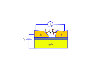
Figure 1: Schematic picture of the physical setup described by the model. The central region (molecule/quantum dot) is coupled to two superconducting leads and can be independently gated by a gate. Electrons entering the central region experience mutual Coulomb interaction and interact with oscillatory modes — either one distinguished mode such as center-of-mass vibration of the molecule as a whole or many modes due to intramolecular vibrations or substrate phonons acting as a heat bath.

The model Hamiltonian is given by

$$H =H_{0}+H_{T},$$ (1)

where the unperturbed part of the Hamiltonian is

$$H_{0}=H_{L}+H_{R}+H_{M},$$ (2)

with $H_{L,R}$ being the BCS Hamiltonians for the left and right leads, respectively,

$$H_{\alpha} =\sum_{k,\sigma=\uparrow,\downarrow}\varepsilon_{k\alpha}c_{k\alpha\sigma}^{{\dagger}}c_{k\alpha\sigma}-\left(\sum_{k}\Delta_{\alpha}c_{k\alpha\uparrow}^{{\dagger}}c_{-k\alpha\downarrow}^{{\dagger}}+\mathrm{H.c.}\right),$$ (3)

with $\alpha=L,R$, and the complex gap functions defined as $\Delta_{\alpha}=|\Delta_{\alpha}|e^{i\phi_{\alpha}}$. Furthermore, $H_{M}$ describes the central region

$$H_{M}=H_{M0}+H_{\mathrm{vib}}+H_{e-\mathrm{vib}},$$ (4)

where $H_{M0}$ is the Hamiltonian for the electronic degrees of freedom

$$H_{M0}=\xi\sum_{\sigma=\uparrow,\downarrow}d_{\sigma}^{{\dagger}}d_{\sigma}+Un_{\uparrow}n_{\downarrow},$$ (5)

with $d_{\sigma},d_{\sigma}^{\dagger}$ being the operators for the local level, and $n_{\uparrow}$ and $n_{\downarrow}$ the corresponding spin-dependent occupations. We assume that the single-particle energy level $\xi$ can be experimentally tuned by the gate, i.e., $\xi\equiv\xi(V_{g})$, and present the results for the critical Josephson current as functions of $\xi$. We have here defined the origin (zero) of $\xi$ to be at the Fermi level of the superconducting electrodes. $H_{\mathrm{vib}}$ is the Hamiltonian for the vibrational degrees of freedom

$$H_{\mathrm{vib}}=\sum_{\nu}\left(\frac{p^{2}}{2m_{\nu}}+\frac{1}{2}m_{\nu}\omega_{\nu}^{2}x_{\nu}^{2}\right)=\sum_{\nu}\omega_{\nu}\left(a^{\dagger}_{\nu}a_{\nu}+\frac{1}{2}\right),$$ (6)

and, finally, $H_{e-\mathrm{vib}}$ describes the coupling between electronic and vibrational degrees of freedom. This coupling is solely through the charge on the central system, i.e.,

$$H_{e-\mathrm{vib}}=(n_{\uparrow}+n_{\downarrow})X,$$ (7)

where

$$X=\sum_{\nu}\lambda_{\nu}x_{\nu}.$$ (8)

In this model we neglect any modification of the tunneling due to the vibrations (this is very often the relevant situation and the model could easily be generalized to incorporate such a dependence), and the tunneling Hamiltonian is therefore given by

$$H_{T}=\sum_{\alpha=L,R}(H_{T\alpha}^{+}+H_{T\alpha}^{-}),$$ (9)

where $H_{T\alpha}^{+}=\left(H_{T\alpha}^{-}\right)^{\dagger}$ and

$$H_{T\alpha}^{-}=\sum_{\sigma=\uparrow,\downarrow}H_{T\alpha\sigma}^{-},\quad H_{T\alpha\sigma}^{-}=\sum_{k}t_{k\alpha}c_{k\alpha\sigma}^{\dagger}d_{\sigma}.$$ (10)

In the next section we will calculate the Josephson coupling using perturbation theory in the tunneling. For this purpose, it is convenient first to use a polaron representation, which transforms the coupling term $H_{e-\mathrm{vib}}$ to a displacement operator in the tunneling term.Mahan (1990); Braig and Flensberg (2003)

The unitary transformation

$$\tilde{H}=SHS^{\dagger},\quad S=e^{-iA(n_{\downarrow}+n_{\uparrow})},$$ (11)

where

$$A=\sum_{\nu}\ell_{\nu}p_{\nu},\quad\ell_{\nu}=\frac{\lambda_{\nu}}{m_{\nu}\omega_{\nu}^{2}},$$ (12)

removes the coupling term $H_{e-\mathrm{vib}}$ from the Hamiltonian at the expense that the tunneling term acquires an oscillator displacement operator, so that Eq. (10) becomes

$$\tilde{H}_{T\alpha\sigma}^{-}=SH_{T\alpha\sigma}^{-}S^{\dagger}=\sum_{k}t_{k\alpha}c_{k\alpha\sigma}^{\dagger}d_{\sigma}e^{iA}.$$ (13)

Furthermore, the transformation renormalizes the on-site energy and the Coulomb interaction according to

$$\tilde{\xi}=\xi-\frac{1}{2}\sum_{\nu}\lambda_{\nu}\ell_{\nu},\quad\tilde{U}=U-\sum_{\nu}\lambda_{\nu}\ell_{\nu}.$$ (14)

In the following we will skip the tildes and use just $\xi,U$ again but we mean the renormalized quantities. Using this transformed Hamiltonian, we calculate the Josephson current to the lowest order in the tunneling Hamiltonian in the following sections.

III Josephson current

The current operator for the current through contact $\alpha=L,R$ is $\dot{N}_{\alpha}$ (we use $\hbar=e=1$ throughout the whole paper), where $N_{\alpha}$ is the operator of the number of electrons in lead alpha. After the unitary polaron transformation introduced previously, we hence obtain the current, $I_{\alpha}$, as

$$I_{\alpha}=i\left\langle\left[\tilde{H},N_{\alpha}\right]\right\rangle=i\left\langle\tilde{H}_{T\alpha}^{+}-\tilde{H}_{T\alpha}^{-}\right\rangle=2\,\mathrm{Im}\,\left\langle\tilde{H}_{T\alpha}^{-}\right\rangle.$$ (15)

Performing the standard thermodynamic perturbation expansionMahan (1990); Bruus and Flensberg (2004) in the tunneling we obtain for the Josephson current in the lowest non-vanishing order, which is the fourth order, in $\tilde{H}_{T}$

$$\begin{split}I_{\alpha}&=-2\,\mathrm{Im}\,\frac{1}{3!}\int_{0}^{\beta}d\tau_{1}\int_{0}^{\beta}d\tau_{2}\int_{0}^{\beta}d\tau_{3}\\ &\quad\times\left\langle T_{\tau}\left(\tilde{H}_{T}(\tau_{1})\tilde{H}_{T}(\tau_{2})\tilde{H}_{T}(\tau_{3})\tilde{H}_{T\alpha}^{-}\right)\right\rangle_{0}.\end{split}$$ (16)

The Josephson current must involve two $\tilde{H}_{T}^{+}$ and two $\tilde{H}_{T}^{-}$, which can be chosen in three ways, and hence

$$\begin{split}I_{\alpha}&=-\mathrm{Im}\,\int_{0}^{\beta}d\tau_{1}\int_{0}^{\beta}d\tau_{2}\int_{0}^{\beta}d\tau_{3}\\ &\quad\times\left\langle T_{\tau}\left(\tilde{H}_{T\bar{\alpha}}^{+}(\tau_{1})\tilde{H}_{T\bar{\alpha}}^{+}(\tau_{2})\tilde{H}_{T\alpha}^{-}(\tau_{3})\tilde{H}_{T\alpha}^{-}\right)\right\rangle_{0},\end{split}$$ (17)

where we also used that in order to have Cooper pair tunneling, the $\tilde{H}_{T}^{+}$ must belong to the junction opposite to where the Josephson current is “measured” via $\tilde{H}_{T\alpha}^{-}$, i.e., $\bar{\alpha}$ means the lead opposite to $\alpha$. Because of spin symmetry we can choose the spin of the last $\tilde{H}_{T}^{-}$ as, say, spin up, which then means that the other $\tilde{H}_{T}^{-}$ carries spin down. In the same way, the spin of the two $\tilde{H}_{T}^{+}$ can be chosen in two ways. All in all, we thus obtain

$$\begin{split}I_{\alpha}&=-4\,\mathrm{Im}\,\int_{0}^{\beta}d\tau_{1}\int_{0}^{\beta}d\tau_{2}\int_{0}^{\beta}d\tau_{3}\\ &\quad\times\left\langle T_{\tau}\left(\tilde{H}_{T\bar{\alpha}\downarrow}^{+}(\tau_{1})\tilde{H}_{T\bar{\alpha}\uparrow}^{+}(\tau_{2})\tilde{H}_{T\alpha\downarrow}^{-}(\tau_{3})\tilde{H}_{T\alpha\uparrow}^{-}\right)\right\rangle_{0}\\ &=-4\,\mathrm{Im}\,\sum_{k}\sum_{p}t_{p\bar{\alpha}}^{\ast}t_{-p\bar{\alpha}}^{\ast}t_{-k\alpha}t_{k\alpha}\int_{0}^{\beta}d\tau_{1}\int_{0}^{\beta}d\tau_{2}\int_{0}^{\beta}d\tau_{3}\\ &\quad\times\mathcal{F}_{k\alpha}(\tau_{3})\mathcal{F}_{p\bar{\alpha}}^{\ast}(\tau_{1}-\tau_{2})\mathcal{B}(\tau_{1},\tau_{2},\tau_{3})\,\mathcal{D}(\tau_{1},\tau_{2},\tau_{3}),\end{split}$$ (18)

where $\mathcal{F}$ are the anomalous Green’s functions of the leads

$$\mathcal{F}_{k\alpha}(\tau)=-\left\langle T_{\tau}\left(c^{\dagger}_{-k\alpha\downarrow}(\tau)c^{\dagger}_{k\alpha\uparrow}(0)\right)\right\rangle_{0}$$ (19)

and where we define the following two functions pertaining to the central region:

$$\mathcal{B}(\tau_{1},\tau_{2},\tau_{3})=\left\langle T_{\tau}\left(d_{\downarrow}^{\dagger}(\tau_{1})d_{\uparrow}^{\dagger}(\tau_{2})d_{\downarrow}(\tau_{3})d_{\uparrow}(0)\right)\right\rangle_{0}$$ (20)

and

$$\mathcal{D}(\tau_{1},\tau_{2},\tau_{3})=\left\langle T_{\tau}\left(e^{-iA(\tau_{1})}e^{-iA(\tau_{2})}e^{iA(\tau_{3})}e^{iA}\right)\right\rangle_{0}.$$ (21)

The first function $\mathcal{B}$ describes the propagation of a Cooper pair through the central region, while the other function $\mathcal{D}$ accounts for the corresponding shifts of the oscillator degrees of freedom when the charge on the central region is changed.

The anomalous Green’s functions $\mathcal{F}$ are easily calculated in the standard way,Mahan (1990); Bruus and Flensberg (2004) and we have

$$\mathcal{F}_{k\alpha}(\tau)=\frac{\Delta_{\alpha}^{*}}{2E_{k\alpha}}f_{\alpha}(E_{k\alpha},\tau),$$ (22)

where

$$f_{\alpha}(E_{k\alpha},\tau)=e^{-E_{k\alpha}|\tau|}-2\cosh\left(E_{k\alpha}\tau\right)n_{F}(E_{k\alpha})$$ (23)

and as usual $E_{k\alpha}=\sqrt{\varepsilon_{k\alpha}^{2}+|\Delta_{\alpha}|^{2}}$. Throughout, we will assume low temperatures such that $|\Delta_{L,R}|\beta\gg 1$, and we can thus approximate

$$f_{\alpha}(E_{k\alpha},\tau)\approx e^{-E_{k\alpha}|\tau|}-e^{-E_{k\alpha}(\beta-|\tau|)}.$$ (24)

In expression (18) for the current there are two sums over states in the superconductors, which define the tunneling density of states (TDOS) as

$$\Gamma_{\alpha}(\varepsilon)\equiv 2\pi\sum_{k}t_{k\alpha}t_{-k\alpha}\delta(\varepsilon-\varepsilon_{k\alpha})=2\pi\sum_{k}|t_{k\alpha}|^{2}\delta(\varepsilon-\varepsilon_{k\alpha}).$$ (25)

For a small central region, where the coupling is point-like, we can approximate $t_{k}$ by a constant, which gives a weak energy dependence of $\Gamma$.

III.1 Critical current

The Josephson current is a function of the phase-difference between the two superconductors and using Eqs. (18), (22), and (25), we have

$$I_{\alpha}=I_{c}\sin\theta,$$ (26)

where the phase difference $\theta=\phi_{\bar{\alpha}}-\phi_{\alpha}$. Finally, the critical current $I_{c}$ is given by

$$\begin{split}I_{c}&=-\frac{1}{\pi^{2}}\int_{0}^{\beta}d\tau_{1}\int_{0}^{\beta}d\tau_{2}\int_{0}^{\beta}d\tau_{3}\int_{-\infty}^{\infty}d\varepsilon\int_{-\infty}^{\infty}d\varepsilon^{\prime}\\ &\quad\times\Gamma_{L}(\varepsilon)\Gamma_{R}(\varepsilon^{\prime})\frac{|\Delta_{L}\Delta_{R}|}{4EE^{\prime}}f_{L}(E,\tau_{3})f_{R}(E^{\prime},\tau_{1}-\tau_{2})\\ &\quad\times\mathcal{B}(\tau_{1},\tau_{2},\tau_{3})\,\mathcal{D}(\tau_{1},\tau_{2},\tau_{3}).\end{split}$$ (27)

This expression forms the basis for the further calculations in this paper. In fact, from now on we will assume that the two tunneling densities of states are energy independent.

The value of $I_{c}$ may come out negative and we will see in the following that it really does so due to the Coulomb interaction. The case with $I_{c}<0$ is called a $\pi$ junction. This terminology originates from an equivalent description of the Josephson junction in terms of total energy (or free energy at nonzero temperature) of the junction as a function of the phase difference $E(\theta)$. Since $I_{\alpha}=2dE(\theta)/d\theta$ the total energy reads $E(\theta)=-(I_{c}/2)\cos\theta$ and reaches minimum at $\theta=0$ for $I_{c}>0$ or $\theta=\pi$ for $I_{c}<0$, respectively (i.e., the ground state of the junction corresponds to equal/opposite phases in the two leads). The $\pi$ junction behavior has been noted in a number of papers. Shiba and Soda (1969); Glazman and Matveev (1989); Spivak and Kivelson (1991); Ishizaka et al. (1995); Clerk and Ambegaokar (2000); Rozhkov et al. (2001); Vecino et al. (2003); Siano and Egger (2004); Zaikin (2004) The origin of this sign change is the blocking of channels for the Cooper pair exchange when $U$ is large. See Ref. Spivak and Kivelson, 1991 for a detailed account.

Ideally the Josephson current can be measured in a current-bias setup where there is no voltage drop across the junction until the critical current is reached. However, in practice current-bias is difficult to achieve for large resistance junctions such as these single-electron devices and instead a voltage is swept across the junction and the critical current must be determined as half of the area of the (ideally $\delta$-function-like) peak in the $dI/dV$curve around $V=0$, which then, of course, only yields the absolute value of $I_{c}$.

III.2 Function $\mathcal{B}$

Since the central region has interactions, we cannot use Wick’s theorem, and we must evaluate the function $\mathcal{B}$ using the many-body states, of which there are four: $|0\rangle,|\!\!\uparrow\rangle,|\!\!\downarrow\rangle,$ and $|\!\!\uparrow\downarrow\rangle.$ In Eq. (20) only $|\!\!\uparrow\rangle$ and $|\!\!\uparrow\downarrow\rangle$ contribute to the trace, i.e., $\mathcal{B}=\mathcal{B}_{1}+\mathcal{B}_{2}$, where

$$\mathcal{B}_{1} =P_{\uparrow}\left\langle\uparrow\!\left|T_{\tau}\left(d_{\downarrow}^{\dagger}(\tau_{1})d_{\uparrow}^{\dagger}(\tau_{2})d_{\downarrow}(\tau_{3})d_{\uparrow}(0)\right)\right|\!\uparrow\right\rangle_{0},$$ (28a)

$$\mathcal{B}_{2} =P_{\uparrow\downarrow}\left\langle\uparrow\downarrow\!\left|T_{\tau}\left(d_{\downarrow}^{\dagger}(\tau_{1})d_{\uparrow}^{\dagger}(\tau_{2})d_{\downarrow}(\tau_{3})d_{\uparrow}(0)\right)\right|\!\uparrow\downarrow\right\rangle_{0},$$ (28b)

with

$$P_{\uparrow} =P_{\downarrow}=\frac{e^{-\beta\xi}}{1+2e^{-\beta\xi}+e^{-\beta E_{2}}},$$ (29a)

$$P_{\uparrow\downarrow} =\frac{e^{-\beta E_{2}}}{1+2e^{-\beta\xi}+e^{-\beta E_{2}}},$$ (29b)

and $E_{2}=2\xi+U$. For $B_{1}$ only three orderings of the operators give a nonzero result, and we find

$$\begin{split}\mathcal{B}_{1}&=P_{\uparrow}\left\{e^{\xi(\tau_{1}-\tau_{3}+\tau_{2})}\theta(\tau_{2}-\tau_{3})\theta(\tau_{3}-\tau_{1})\right.\\ &\quad+e^{E_{2}(\tau_{2}-\tau_{3})}e^{\xi(\tau_{1}-\tau_{2}+\tau_{3})}\theta(\tau_{3}-\tau_{2})\theta(\tau_{2}-\tau_{1})\\ &\quad+\left.e^{E_{2}(\tau_{1}-\tau_{3})}e^{\xi(\tau_{2}-\tau_{1}+\tau_{3})}\theta(\tau_{3}-\tau_{1})\theta(\tau_{1}-\tau_{2})\right\}.\end{split}$$ (30)

Likewise, for $B_{2}$ we find

$$\begin{split}\mathcal{B}_{2}&=-P_{\uparrow\downarrow}\left\{e^{\xi(\tau_{2}-\tau_{3}-\tau_{1})}e^{E_{2}\tau_{1}}\theta(\tau_{1}-\tau_{2})\theta(\tau_{2}-\tau_{3})\right.\\ &\quad+e^{\xi(\tau_{1}-\tau_{2}-\tau_{3})}e^{E_{2}\tau_{2}}\theta(\tau_{2}-\tau_{1})\theta(\tau_{1}-\tau_{3})\\ &\quad\left.+e^{(E_{2}-\xi)(\tau_{1}+\tau_{2}-\tau_{3})}\theta(\tau_{1}-\tau_{3})\theta(\tau_{3}-\tau_{2})\right\}.\end{split}$$ (31)

III.3 Function $\mathcal{D}$

We also calculate the function $\mathcal{D}$ in Eq. (21) involving the bosonic degrees of freedom. Since the unperturbed Hamiltonian is quadratic in boson operators, this is evaluated asMahan (1990)

$$\begin{split}\mathcal{D}=\exp\Big{(}&h(\tau_{1}-\tau_{3})+h(\tau_{1})+h(\tau_{2}-\tau_{3})+h(\tau_{2})\\ &-h(\tau_{1}-\tau_{2})-h(\tau_{3})\Big{)},\end{split}$$ (32)

where the function $h$ is defined as

$$h(\tau)=\left\langle T_{\tau}\big{(}A(\tau)A(0)\big{)}\right\rangle_{0}-\left\langle A^{2}\right\rangle_{0}.$$ (33)

When inserting the formula (12) for the operator $A$ one obtains

$$\begin{split}h(\tau)&=\int_{0}^{\infty}d\omega\frac{J(\omega)}{\omega^{2}}\left(n_{B}(\omega)(e^{\omega|\tau|}-1)\right.\\ &\qquad\qquad\qquad\ \left.+(1+n_{B}(\omega))(e^{-\omega|\tau|}-1)\right),\end{split}$$ (34)

with the spectral function of the bath $J(\omega)$

$$J(\omega)=\sum_{\nu}\frac{\lambda_{\nu}^{2}}{2m_{\nu}\omega_{\nu}}\,\delta(\omega-\omega_{\nu}),$$ (35)

and the Bose function $n_{B}(\omega)$

$$n_{B}(\omega)=\frac{1}{\exp(\beta\omega)-1}.$$ (36)

In this paper, we concentrate on two cases — either a single important vibrational mode or a bath of harmonic modes. For the latter case, we consider mainly the situation where the dispersion relation corresponds to the so-called Ohmic case, equivalent to a frequency independent damping coefficient or, equally, spectral function $J(\omega)$ linear in frequency.

III.3.1 Single oscillator case

The case of a single oscillator with frequency $\omega_{0}$, mass $m$ and coupling constant $\lambda$ corresponds to $J_{\mathrm{osc}}(\omega)=g\omega_{0}^{2}\delta(\omega-\omega_{0})$, where the dimensionless $g=\lambda^{2}/2m\omega_{0}^{3}$ as in Ref. Braig and Flensberg, 2003, and we have

$$h_{\mathrm{osc}}(\tau)=g\big{[}n_{0}(e^{\omega_{0}|\tau|}-1)+(1+n_{0})(e^{-\omega_{0}|\tau|}-1)\big{]},$$ (37)

with $n_{0}=n_{B}(\omega_{0})$.

III.3.2 Ohmic environment case

The other generic case that we consider is that of Ohmic heat bath in which case we use the spectral function

$$J_{\mathrm{ohm}}(\omega)=g\omega\exp(-\omega/\omega_{c})$$ (38)

parametrized by the dimensionless interaction constant $g$ and the upper cutoff frequency $\omega_{c}$. In this important case it is possible to calculate at $T=0$ the correlation function $h(\tau)$ from Eq. (34) analytically yielding

$$h_{\mathrm{ohm}}(\tau)=-g\ln(1+\omega_{c}|\tau|)\ .$$ (39)

IV Josephson current without dissipation

As a reference for the discussion on the influence of coupling to a dissipative environment, we discuss the case without coupling to the bosonic environment. This we do in three steps: first we set $U=0$, then we look at the infinite $U$ case and finally we give the expression for the general case.

IV.1 No Coulomb interaction $U=0$

This result is derived in Appendix A, and the critical current is found to be

$$I_{c}(\xi)=\frac{\Gamma_{L}\Gamma_{R}}{2(1-(\xi/\Delta)^{2})}\Big{(}\frac{\tanh(\beta\xi/2)}{\xi}-\frac{\tanh(\beta\Delta/2)}{\Delta}\Big{)}.$$ (40)

We note that this expression diverges when $\xi=0$ and $T=0$, which however is regularized by higher order terms in $\Gamma$’s, see discussion in Appendix A. Furthermore, we see that the critical current is always positive, which means that the negative critical currents, i.e., the $\pi$ junction behavior, found below are a result of the correlations. In Fig. 2 this noninteracting result is compared with two interacting cases $U=\Delta$ and $U\to\infty$.

IV.2 Strong Coulomb interaction $U\to\infty$

Let $U\to\infty$ such that the doubly occupied state is taken out. Hence

$$\mathcal{B}_{1}=P_{\uparrow}e^{\xi(\tau_{1}-\tau_{3}+\tau_{2})}\theta(\tau_{2}-\tau_{3})\theta(\tau_{3}-\tau_{1})\,\,,$$ (41)

and when inserting this into formula for the critical current (27), performing the imaginary time integrations using the approximation (24) and $\beta\Delta\gg 1$ (so that $\exp(-\beta E_{k\alpha})\approx 0$), we findGlazman and Matveev (1989); Ishizaka et al. (1995); Rozhkov et al. (2001)

$$I_{c}(\xi)=\frac{\Gamma_{L}\Gamma_{R}}{\pi^{2}}N(\xi)$$ (42)

where

$$N(\xi)\!=-\!\!\int_{|\Delta_{L}|}^{\infty}\frac{|\Delta_{L}|dE}{\sqrt{E^{2}-|\Delta_{L}|^{2}}}\int_{|\Delta_{R}|}^{\infty}\frac{|\Delta_{R}|dE^{\prime}}{\sqrt{E^{\prime 2}-|\Delta_{R}|^{2}}}\,C(E,E^{\prime})$$ (43)

and

$$\begin{split}C(E,E^{\prime})&\!=\!\frac{2e^{-\beta\xi}}{1+2e^{-\beta\xi}}\left(-\frac{e^{\beta\xi}}{(E+E^{\prime})\left(E+\xi\right)\left(E^{\prime}+\xi\right)}\right.\\ &\left.\quad+\frac{1}{(E+E^{\prime})\left(E-\xi\right)\left(E^{\prime}-\xi\right)}\right).\end{split}$$ (44)

At $T=0,$ this reduces to

$$C(E,E)=\left\{\begin{array}[]{cc}-2\left[(E+E^{\prime})(E+\xi)(E^{\prime}+\xi)\right]^{-1}&\mathrm{for}\,\xi>0,\\[5.69054pt] \left[(E+E^{\prime})(E-\xi)(E^{\prime}-\xi)\right]^{-1}&\mathrm{for}\,\xi<0.\end{array}\right.$$ (45)

The integral in Eq. (43) can be performed analytically at $T=0$, and $|\Delta_{L}|=|\Delta_{R}|=\Delta$ yielding

$$N(\xi)=\left\{\begin{array}[]{cc}2\,n(\xi/\Delta)/\Delta&\mathrm{for}\quad\xi>0,\\[5.69054pt] -n(-\xi/\Delta)/\Delta&\mathrm{for}\quad\xi<0.\end{array}\right.$$ (46)

The dimensionless function $n(x)$ defined as ($x>-1$)

$$n(x)\!=\!\int_{1}^{\infty}\!\frac{du}{\sqrt{u^{2}-1}}\int_{1}^{\infty}\!\frac{dv}{\sqrt{v^{2}-1}}\frac{1}{(u+v)(u+x)(v+x)},$$ (47)

can be expressed by (see Appendix B)

$$n(x)=\frac{\frac{\pi^{2}}{4}(1-x)-\arccos^{2}x}{x(1-x^{2})},\quad\text{with }\,-1<x,$$ (48)

where the analytic continuations of $\arccos x=i\ln(x+\sqrt{x^{2}-1})$ for $x>1$ is understood. The function $n(x)$ is always positive, it diverges at $x\to-1^{+}$, and then smoothly decays for increasing $x$ with the asymptote $n(x)\sim\pi^{2}/4x^{2}$ for $x\to\infty$. The expression (46) is compared with the noninteracting and finite $U$ results in Fig. 2. We see that the magnitude of the critical current is highly suppressed by the very strong Coulomb interaction.

For finite but small temperatures $\beta\Delta\gtrsim 10$ so that our approximations are still valid, we can write for the magnitude of the Josephson current (for $|\xi|<\Delta$ only, otherwise the zero temperature expression should be used)

$$I_{c}(\xi)=\frac{2\Gamma_{L}\Gamma_{R}}{\pi^{2}\Delta}\frac{n(\xi/\Delta)-e^{-\beta\xi}n(-\xi/\Delta)}{(1+2e^{-\beta\xi})}.$$ (49)

The finite temperature behavior in the limit $U\to\infty$ is illustrated in more detail in Fig. 3 for three values of temperature. In the lowest temperature curve $\beta\Delta=10$ we also compare the analytic expression (49) with a direct numerical evaluation of the triple imaginary-time integral (Eq. (53) with $\mathcal{D}\equiv 1$) routinely used for the dissipative cases. We see an excellent agreement between the two methods.

In an experiment with a single Josephson junction the absolute values of the presented curves would be measured. This would give curves with a dip down to zero at $\xi=0$ (for a finite temperature) and with asymmetric shoulders around the dip with the ratio between the shoulder heights being 2. Even though the dip may be smeared in the experiment for low enough temperatures the asymmetric shoulders should persist thus revealing the crossover to the $\pi$ junction regime.

IV.3 Finite Coulomb interaction $U$

For a finite value of $U$ we have to consider all terms of $B=B_{1}+B_{2}$ in an analogous way as previously the first one in the $U\to\infty$ case. Neglecting again terms $e^{-\beta E_{k,p}}$, we recover the formula (42) for the current, but with the function $C(E,E^{\prime})$ in Eq. (43) replaced by

$$C(E,E^{\prime})=\frac{2}{Z(E+E^{\prime})}L(E,E^{\prime}),$$ (50)

where $Z=\big{(}1+2e^{-\beta\xi}+e^{-\beta(2\xi+U)}\big{)}$ and

$$\begin{split}L(E,E^{\prime})&=-\frac{1}{(E+\xi)(E^{\prime}+\xi)}+\frac{e^{-\beta\xi}}{(E-\xi)(E^{\prime}-\xi)}\\ &\quad+\frac{2\,e^{-\beta(2\xi+U)}(E+E^{\prime})}{(2\xi+U)(\xi+U-E)(\xi+U-E^{\prime})}\\ &\quad-\frac{2(E+E^{\prime})}{(2\xi+U)(\xi+E)(\xi+E^{\prime})}\\ &\quad+\frac{2e^{-\beta\xi}}{(E^{\prime}-\xi)(E^{\prime}+\xi+U)}\\ &\quad+\frac{2e^{-\beta\xi}}{(E-\xi)(E+\xi+U)}\\ &\quad+\frac{e^{-\beta\xi}}{(E+\xi+U)(E^{\prime}+\xi+U)}\\ &\quad-\frac{e^{-\beta(2\xi+U)}}{(\xi+U-E)(\xi+U-E^{\prime})}.\end{split}$$ (51)

The resulting integral does not seem to be analytically calculable in the whole $\xi$-range, not even at $T=0$ and $|\Delta_{L}|=|\Delta_{R}|=\Delta$. Yet, in that limit one can achieve significant simplifications at least for some $\xi$’s which even allow us to evaluate the $n(x)$ function defined by Eq. (47) yielding Eq. (48). The details of those calculations can be found in Appendix B. We have, however, calculated the critical current numerically, and an example is shown in Fig. 2 for $U=\Delta$.

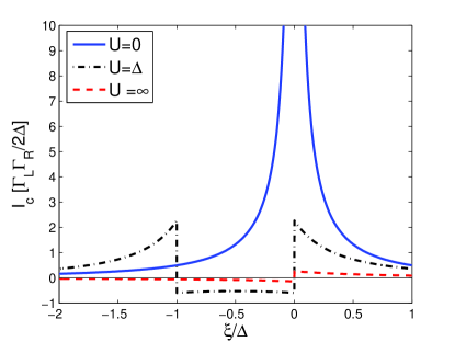
Figure 2: (Color online) Josephson current dependence on the Coulomb interaction strength at zero temperature. Shown are the critical Josephson current through an Anderson level with no Coulomb interaction $U=0$ (full line), with moderate interaction $U=\Delta$ (dash-dotted line), and with infinite repulsion $U\to\infty$ (dashes). The interacting cases exhibit the phenomenon of the $\pi$ junction for $-U<\xi<0$, but the overall magnitude of the current decreases largely with the increasing interaction strength.

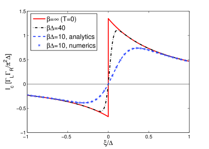
Figure 3: (Color online) Josephson current dependence on the temperature for $U\to\infty$. We show the temperature dependence of the critical Josephson current for $|\xi|<\Delta$ for three different temperatures $T=0\ (\beta\to\infty)$ (full line), $\beta\Delta=40$ (dash-dotted line), and $\beta\Delta=10$ (dashed line with asterisks). In the last case which illustrates roughly the highest temperature achievable within the approximations used the analytic and numerical results are compared.

V Josephson current with dissipation

Next, we study how the critical Josephson current changes, when coupling to vibrational modes is included. In order to do that, we will perform a numerical integration of the three imaginary time integrals. For this purpose we first find (again assuming $\Gamma_{\alpha}(\varepsilon)$ constant)

$$\begin{split}\mathcal{H}_{\alpha}(\tau)&\equiv\int_{|\Delta_{\alpha}|}^{\infty}dE\frac{1}{\sqrt{E^{2}-|\Delta_{\alpha}|^{2}}}\left[e^{-E|\tau|}-e^{-E(\beta-|\tau|)}\right]\\ &=K_{0}(|\tau\Delta_{\alpha}|)-K_{0}((\beta-|\tau|)|\Delta_{\alpha}|),\end{split}$$ (52)

where $K_{0}(x)$ is the modified Bessel function of the second kind. The expression for the critical current thus reads

$$\begin{split}I_{c}&=-\frac{\Gamma_{L}\Gamma_{R}|\Delta_{L}\Delta_{R}|}{\pi^{2}}\int_{0}^{\beta}d\tau_{1}\int_{0}^{\beta}d\tau_{2}\int_{0}^{\beta}d\tau_{3}\,\mathcal{H}_{L}(\tau_{1}-\tau_{2})\\ &\quad\times\mathcal{H}_{R}(\tau_{3})\mathcal{B}(\tau_{1},\tau_{2},\tau_{3})\mathcal{D}(\tau_{1},\tau_{2},\tau_{3}).\end{split}$$ (53)

We evaluated $I_{c}$ numerically for a number of different cases with the qualitatively same results showing that the coupling to oscillator mode(s) suppresses the magnitude of the Josephson current. There is no apparent difference between the single mode and Ohmic heat bath case which is in a clear contrast with nonequilibrium transport studies where the character of the phonon spectrum plays a crucial role in the current-voltage characteristics. Below, just for simplicity, we only present results for the symmetric case $|\Delta_{L}|=|\Delta_{R}|=\Delta$ at zero temperature $T=0$ and for infinite Coulomb interaction $U\to\infty$.

V.1 Low-frequency phonons

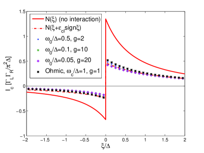
Figure 4: (Color online) Josephson current for low-frequency phonons at $T=0,\,U\to\infty$. As long as the spectrum of the phonon mode(s) is well below the superconducting gap, i.e., $\omega_{0,c}\ll\Delta$, the critical Josephson current only depends on the integral $\varepsilon_{\rm cl}=\int_{0}^{\infty}d\omega J(\omega)/\omega=g\omega_{0,c}$ via the shifted dissipationless function $N(\xi+\varepsilon_{\rm cl}\,\mathrm{sgn}\xi)$ (dash-dotted line). Numerical results are shown for a single phonon mode with $\omega_{0}=0.5\Delta,\,g=2$ (dots), $\omega_{0}=0.1\Delta,\,g=10$ (asterisks), $\omega_{0}=0.05\Delta,\,g=20$ (pluses), and for the Ohmic bath with $\omega_{c}=\Delta,\,g=1$ (crosses). All of these cases yield basically the same result very well captured by the analytic expression.

If the spectrum of the oscillator mode(s) is well below the superconducting gap $\omega_{0,c}\ll\Delta$ we can find an approximate analytic expression for the $I_{c}(\xi)$ with the help of the function $n(\xi)$ of the $U\to\infty$ case with no phonons, Eq. (48). To this end we study the current formula (53) when we plug into it the expressions for $\mathcal{B}(\tau_{1},\tau_{2},\tau_{3})$ (41) and $\mathcal{D}(\tau_{1},\tau_{2},\tau_{3})$ (32) and consider the above limit. For $\xi\leq 0$ we notice that the step functions of Eq. (41) and the fast decaying functions $\mathcal{H}_{\alpha}(\tau)$ in Eq. (53) limit the relevant contributions to the three-dimensional integral to values of $\tau_{1},\tau_{2},\tau_{3}$ small compared to $\min\{1/|\xi|,1/\Delta\}$. For that reason one can perform the Taylor expansion in Eq. (32) of the $h(\tau)$ functions given by Eq. (34) which gives

$$h(\tau)\approx-|\tau|\,\int_{0}^{\infty}d\omega\,\frac{J(\omega)}{\omega}\equiv-\varepsilon_{\rm cl}|\tau|,$$ (54)

where we have defined the quantity

$$\varepsilon_{\rm cl}=\int_{0}^{\infty}d\omega\,\frac{J(\omega)}{\omega}=\sum_{\nu}\frac{\lambda_{\nu}^{2}}{2m_{\nu}\omega_{\nu}^{2}}=\sum_{\nu}\frac{1}{2}m_{\nu}\omega_{\nu}^{2}l_{\nu}^{2},$$ (55)

being the classical displacement energy when the oscillators are displaced by $l_{\nu}$ due to the force generated by a single excess electron. Putting the expansion into Eqs. (32) and (53) we get

$$\begin{split}I_{c}(\xi)&=-\frac{\Gamma_{L}\Gamma_{R}\Delta^{2}}{\pi^{2}}\frac{e^{-\beta\xi}}{1+2e^{-\beta\xi}}\int_{0}^{\beta}d\tau_{2}\int_{0}^{\tau_{2}}d\tau_{3}\int_{0}^{\tau_{3}}d\tau_{1}\\ &\quad\times\mathcal{H}_{L}(\tau_{1}-\tau_{2})\mathcal{H}_{R}(\tau_{3})\,e^{(\xi-\varepsilon_{\rm cl})(\tau_{1}-\tau_{3}+\tau_{2})},\end{split}$$ (56)

valid for $\text{ for }\xi\leq 0$. This in fact corresponds to the dissipationless case with the replacement $\xi\to\xi-\varepsilon_{\rm cl}$. In particular, in the zero temperature limit we get $I_{c}(\xi)=-(\Gamma_{L}\Gamma_{R}/\pi^{2}\Delta)n[(\xi-\varepsilon_{\rm cl})/\Delta]$ for $\xi\leq 0$. For $\xi\geq 0$ we have to combine the vanishing prefactor $\exp(-\beta\xi)$ with the divergent integral (for $\beta\to\infty$) to get a finite result. This can be done by the substitutions $\tau_{i}^{\prime}=\beta-\tau_{i},\ i=1,2,3$ which make the integrand relevant only for small values of $\tau_{i}^{\prime}$’s and, analogously to the previous derivation, one finally finds in the zero temperature limit, that $I_{c}(\xi)=(2\Gamma_{L}\Gamma_{R}/\pi^{2}\Delta)n[(\xi+\varepsilon_{\rm cl})/\Delta]$ valid for $\xi\geq 0$. In total, the critical Josephson current in case of coupling to low-frequency oscillator modes can be expressed as (remember the relation (46) between $N(\xi)$ and $n(x)$)

$$I_{c}(\xi)=\frac{\Gamma_{L}\Gamma_{R}}{\pi^{2}\Delta}N(\xi+\varepsilon_{\rm cl}\,\mathrm{sgn}\xi).$$ (57)

This result is illustrated in detail in Fig. 4.

We point out that even in case of finite temperature there is no residual temperature dependence due to coupling to the bath even though the low-frequency modes could be significantly populated. This is seen from the expansion (54) where the thermal occupation factors $n_{B}(\omega)$ cancelled out. Thus, the only temperature dependence would be the one stemming from the occupation factors exactly as in the dissipationless case, Eq. (49) and Fig. 3.

V.2 High-frequency single oscillator mode

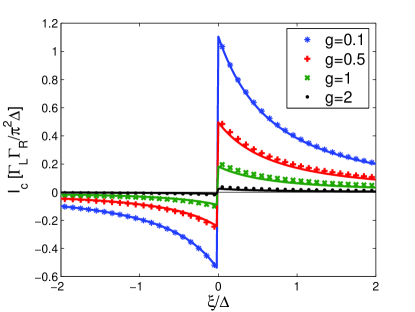
Figure 5: (Color online) Josephson current for high-frequency single oscillator at $T=0,\,U\to\infty,\omega_{0}=20\Delta$. For large enough $\omega_{0}\gg\Delta,\xi$ the Josephson current is expected to be suppressed just by the factor $\exp(-2g)$ compared to the case without the phonon. This is shown in the figure where the numerical results for several values of the coupling constant $g=0.1$ (asterisks), $g=0.5$ (pluses), $g=1$ (crosses), and $g=2$ (dots) are compared with the analytic expressions given by the corresponding lines.

For the high-frequency single phonon mode $\omega_{0}\gg\Delta,\xi$ we expect suppression of the critical Josephson current due to the fact that only transport through the ground oscillator state is allowed since the (virtual) involvement of the excited states would be further suppressed by a factor $\Delta/n\omega_{0}\ll 1\ (n=1,2,3,\dots)$. The transport through the ground state is then diminished by the overlap factors $f_{00}=\langle 0|e^{-il_{0}p_{0}}|0\rangle_{0}$, more precisely the Josephson current should be suppressed by a factor of order

$$|f_{00}|^{4}=\left[\exp\left(-\frac{1}{2}\int_{0}^{\infty}\frac{d\omega}{\omega^{2}}J(\omega)\right)\right]^{4}=e^{-2g}.$$ (58)

At $T=0$ and for $\omega_{0}\gg\Delta,\xi$ the function $h_{\mathrm{osc}}(\tau)=g(e^{-\omega_{0}|\tau|}-1)$ changes very fast for small $\tau$’s of the order $\tau\sim 1/\omega_{0}$ which is irrelevant for the integral (53). For larger $\tau$’s the function $h_{\mathrm{osc}}(\tau)\sim-g$ is constant and thus we get from Eq. (32) that the total effect of the phonon on the Josephson current is just a constant factor of $e^{-2g}$ multiplying the dissipationless case. This effect is shown in Fig. 5 for different values of the coupling constant $g$ at fixed $\omega_{0}=20\Delta$. The results do not depend on the value of $\omega_{0}$ provided it is high enough, which depends on the value of $g$, as expected (not shown). One can see that the approximation gets worse with increased $g$ (for fixed $\omega_{0}$) which can be explained by the increased contribution of higher order virtual processes favored by the larger value of the coupling constant.

V.3 Ohmic bath with high-frequency cutoff

The case of Ohmic bath with large cutoff energy may be the physically most relevant one. Unfortunately, there is no simple semianalytic theory for this case and thus we have to rely mainly on the numerical results which are summarized in Fig. 6. One should notice the very strong dependence on the coupling constant $g$. Even for intermediate coupling strength $g\sim 1$ we get a significant suppression of $I_{c}$.

We can give a qualitative explanation of the strong suppression due to the large frequency part of the phonon spectrum, $\omega>\Delta$. Roughly, we capture the effect of these high-frequency modes by a suppression factor similar to Eq. (58). This factor is estimated as

$$|\tilde{f}_{00}|^{4}\sim\left[\exp\left(-\frac{g}{2}\int_{\Delta}^{\omega_{c}}\frac{d\omega}{\omega}\right)\right]^{4}=\left(\frac{\Delta}{\omega_{c}}\right)^{2g}.$$ (59)

Thus for large $\omega_{c}$ and/or $g$ the supercurrent is suppressed quite severely, in qualitative agreement with the results presented in Fig. 6.

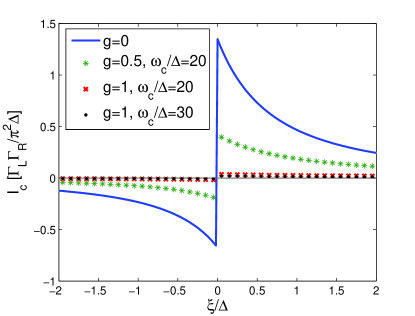
Figure 6: (Color online) Josephson current for high-frequency-cutoff Ohmic bath at $T=0,\,U\to\infty$ and for several values of the coupling constant $g$ and cutoff frequency $\omega_{c}$. We see a significant suppression of the critical current already for intermediate coupling $g=1$.

VI Summary and discussion

We have calculated the Josephson current through a single correlated level with coupling to external bosonic degrees of freedom representing, e.g., a system consisting of a molecular transistor with a number of internal vibrational modes and coupled to the phonons of the substrate.

First, we have studied the case without coupling to vibrations. This situation has been studied previously in a number of papers, but we have derived new analytic formulae. The effect of the Coulomb interaction is to strongly suppress the Josephson current at the charge degeneracy point, and since this is where the junction also crosses over to $\pi$ junction behavior, the critical current in fact goes to zero at this point. One could check this behavior using, e.g., nanotube devices coupled to superconductors as in Refs. Buitelaar et al., 2002, Buitelaar et al., 2003 by tuning the gate voltage across the charge degeneracy point. Also the temperature dependence predicted here could be experimentally verified.

In the second part of the paper we have included the coupling to environmental modes and discussed different limits. Coupling to low-frequency phonons does not have a severe influence on the Josephson coupling, since it only shifts the argument of the dissipationless formula from the single particle energy by the classical displacement energy. In contrast, a strong coupling to high-energy phonons suppresses the supercurrent quite substantially. This is because the oscillators are displaced twice during the transfer of Cooper pair, and because the supercurrent requires the final state of the oscillator to be identical to the initial one, the transfer is suppressed by twice the exponential Franck-Condon factor $e^{-2g}$. Therefore it might be difficult to observe Josephson tunneling current in devices with a strong electron-vibron coupling.

Throughout the paper we have used lowest-order perturbation theory in the tunneling coupling. For stronger tunneling coupling one expects the correlation effect due to the vibrations to become smaller, because the charge on the level is no longer well defined. This means that a mean-field treatment becomes adequate, when $\Gamma>\varepsilon_{\rm cl}$. How to describe this transition theoretically is an interesting problem.

Appendix A Noninteracting case $U=0$

The noninteracting case is exactly solvable for any values of parameters.Beenakker and van Houten (1992); Li et al. (2002) Here, we only give a brief sketch of the solution and the summary of the results in the limit of small $\Gamma$ relevant for our study. Since the model for $U=0$ has a quadratic Hamiltonian, it can be solved by the equation of motion technique for the Matsubara Green function. We introduce an infinite vector $\alpha=(d_{\uparrow},d^{{\dagger}}_{\downarrow},c_{kL\uparrow},c^{{\dagger}}_{-kL\downarrow},c_{kR\uparrow},c^{{\dagger}}_{-kR\downarrow})^{T}$ generalizing the standard Nambu formalism to the case of the dot plus two leads. Defining the corresponding thermal Green function $\mathcal{G}(\tau)=-\langle T_{\tau}(\alpha(\tau)\alpha^{{\dagger}})\rangle$ satisfying the equation of motion $\frac{d}{d\tau}\mathcal{G}(\tau)=-\delta(\tau)\mathrm{1}+\mathrm{M}\cdot\mathcal{G}(\tau)$ with the matrix

$$\mathrm{M}=\begin{pmatrix}-\xi&0&-t_{kL}^{*}&0&-t_{kR}^{*}&0\\ 0&\xi&0&t_{-kL}&0&t_{-kR}\\ -t_{kL}&0&-\varepsilon_{kL}&\Delta_{L}&0&0\\ 0&t_{-kL}^{*}&\Delta_{L}^{*}&\varepsilon_{kL}&0&0\\ -t_{kR}&0&0&0&-\varepsilon_{kR}&\Delta_{R}\\ 0&t_{-kR}^{*}&0&0&\Delta_{R}^{*}&\varepsilon_{kR}\end{pmatrix}$$ (60)

we can express the Josephson current as

$$I_{L}=-4\,\mathrm{Im}\sum_{k}t_{-kL}\mathcal{G}_{42}(\tau\to 0^{+})$$ (61)

(factor of 2 for spin degeneracy). Going to the frequency picture ($\frac{d}{d\tau}\rightarrow-i\omega_{n}$) and using the partitioning scheme

$$\!\!\begin{pmatrix}A&c\\ d&B\end{pmatrix}^{-1}\!\!\!\!=\!\!\begin{pmatrix}(A-cB^{-1}d)^{-1}&-A^{-1}c(B-dA^{-1}c)^{-1}\\ -B^{-1}d(A-cB^{-1}d)^{-1}&(B-dA^{-1}c)^{-1}\end{pmatrix}$$ (62)

together with the wide-band approximation $\Gamma_{\alpha}=\text{const}$, and assuming the symmetric case $\Gamma_{L}=\Gamma_{R}=\Gamma,\,\Delta_{L}=\Delta e^{i\phi},\,\Delta_{R}=\Delta$ this set of linear equations gives for the Josephson current

$$I_{L}=\mathrm{Im}\frac{1}{\beta}\sum_{\omega_{n}}e^{i\omega_{n}0^{-}}\frac{\Gamma^{2}\Delta^{2}e^{-i\phi}}{(\omega_{n}^{2}+\Delta^{2})D(\omega_{n})}$$ (63)

with

$$D(\omega_{n})=\omega_{n}^{2}\Big{(}1+\frac{\Gamma}{\sqrt{\omega_{n}^{2}+\Delta^{2}}}\Big{)}^{2}+\xi^{2}+\frac{\Delta^{2}\Gamma^{2}\cos^{2}(\phi/2)}{(\omega_{n}^{2}+\Delta^{2})}.$$ (64)

The zeros of $D(\omega_{n})$ determine the Andreev bound states discussed in Ref. Vecino et al., 2003. In the limit $\Gamma\to 0$ which we consider here the lowest order contribution to $I_{L}$ is proportional to $\Gamma^{2}$ and can be obtained by setting $\Gamma=0$ in $D(\omega_{n})$. The sum can then be easily performed yielding

$$\ I_{L}=-\sin\phi\frac{\Gamma^{2}}{2(1-(\xi/\Delta)^{2})}\Big{(}\frac{\tanh(\beta\xi/2)}{\xi}-\frac{\tanh(\beta\Delta/2)}{\Delta}\Big{)}.$$ (65)

For $k_{B}T\ll\Delta$ this expression is proportional to $\Gamma^{2}/k_{B}T$ at $\xi=0$. This would diverge in the $T=0$ limit. However, this divergence is just an artifact of our perturbation theory and the exact evaluation of the full expression (63) would give a finite result even at $T=0,\,\xi\to 0$. The exact result is essentially identical to our approximate one unless $\xi,k_{B}T\lesssim\Gamma$ when the exact result gives a saturation of the maximum Josephson currentBeenakker and van Houten (1992); Li et al. (2002) $I_{c}\approx\Gamma$ around $\xi=0$ for $\Gamma\ll\Delta$. For nonsymmetric coupling to the leads, i.e., $\Gamma_{L}\neq\Gamma_{R}$ but still $|\Delta_{L}|=|\Delta_{R}|=\Delta$, we get within the discussed lowest order approximation in $\Gamma$’s the same result just with the replacement $\Gamma^{2}\to\Gamma_{L}\Gamma_{R}$ which is used in the main text, Sec. IV.1.

Appendix B Finite $U$, evaluation of $n(x)$

In this appendix we calculate the critical Josephson current for finite value of the Coulomb interaction $U$ in the limit of zero temperature $T=0$ and symmetric gap $|\Delta_{L}|=|\Delta_{R}|=\Delta$. The critical current is given by Eq. (42) with the function $N(\xi)$ being determined in this case by Eqs. (43), (50), and (51) which further simplify in the considered limit of zero temperature and symmetric gap so that we can write for $N(\xi)$:

$$N(\xi) =\int_{\Delta}^{\infty}dE\int_{\Delta}^{\infty}dE^{\prime}\frac{2\Delta^{2}}{\sqrt{E^{2}-\Delta^{2}}\sqrt{E^{\prime 2}-\Delta^{2}}}\left[\frac{1}{(E+E^{\prime})\left(E+\xi\right)\left(E^{\prime}+\xi\right)}+\frac{2}{(2\xi+U)(\xi+E)(\xi+E^{\prime})}\right]$$

$$=2\left(\frac{n(\xi/\Delta)}{\Delta}+\frac{\arccos^{2}(\xi/\Delta)}{(\xi+U/2)(1-(\xi/\Delta)^{2})}\right)\qquad\mathrm{for}\quad\xi>0,$$ (66a)

$$N(\xi) =-\int_{\Delta}^{\infty}dE\int_{\Delta}^{\infty}dE^{\prime}\frac{\Delta^{2}}{(E+E^{\prime})\sqrt{E^{2}-\Delta^{2}}\sqrt{E^{\prime 2}-\Delta^{2}}}\left[\frac{1}{\left(E-\xi\right)\left(E^{\prime}-\xi\right)}+\frac{1}{(E+\xi+U)(E^{\prime}+\xi+U)}\right.$$

$$\quad+\left.\frac{4}{(E-\xi)(E+\xi+U)}\right]=-\frac{n(-\xi/\Delta)+n((\xi+U)/\Delta)+4n_{2}(-\xi/\Delta,(\xi+U)/\Delta)}{\Delta}\qquad\mathrm{for}\quad-U<\xi<0,$$ (66b)

$$N(\xi) =\int_{\Delta}^{\infty}dE\int_{\Delta}^{\infty}dE^{\prime}\frac{2\Delta^{2}}{\sqrt{E^{2}-\Delta^{2}}\sqrt{E^{\prime 2}-\Delta^{2}}}\left[\frac{1}{(E+E^{\prime})\left(\xi+U-E\right)\left(\xi+U-E^{\prime}\right)}-\frac{2}{(2\xi+U)(\xi+U-E)(\xi+U-E^{\prime})}\right]$$

$$=2\left(\frac{n(|\xi+U|/\Delta)}{\Delta}-\frac{\arccos^{2}(|\xi+U|/\Delta)}{(\xi+U/2)(1-(|\xi+U|/\Delta)^{2})}\right)\qquad\mathrm{for}\quad\xi<-U.$$ (66c)

Here, $n(x)$ is defined by Eq. (47) and

$$\begin{split}n_{2}(x,y)&=\int_{1}^{\infty}\frac{du}{\sqrt{u^{2}-1}}\int_{1}^{\infty}\frac{dv}{\sqrt{v^{2}-1}}\frac{1}{(u+v)(u+x)(u+y)}\\ &=\int_{1}^{\infty}du\frac{\ln(u+\sqrt{u^{2}-1})}{(u^{2}-1)(u+x)(u+y)}.\end{split}$$ (67)

Again, the appropriate analytic continuation of $\arccos x$ for $x>1$ is understood (see discussion below Eq. (48)). While neither of the integral definitions of $n(x)$ (Eq. (47)) or $n_{2}(x,y)$ (Eq. (67)) seems to lead to an explicit formula we still could, however, use the above equations for indirect evaluation of $n(x)$. In particular, since the first equation (66a) is valid for $\xi>0$ for any value of $U$ including both the limits $U\to 0$ and $U\to\infty$ we can use the former limit for the evaluation of the latter one. The noninteracting case $U=0$ is described by Eq. (40) and, thus, we come to the simple result (48) (in the limit $\beta\to\infty$). The function $n_{2}(x,y)$ can be easily calculated by numerical evaluation of the integral in Eq. (67) for $x,y>-1$.

References

- Averin and Nazarov (1992) D. V. Averin and Y. V. Nazarov, Phys. Rev. Lett. 69, 1993 (1992).
- Tuominen et al. (1992) M. T. Tuominen, J. M. Hergenrother, T. S. Tighe, and M. Tinkham, Phys. Rev. Lett. 69, 1997 (1992).
- Shiba and Soda (1969) H. Shiba and T. Soda, Progr. Theor. Phys. 41, 25 (1969).
- Glazman and Matveev (1989) L. I. Glazman and K. A. Matveev, JETP Lett. 49, 659 (1989).
- Spivak and Kivelson (1991) B. I. Spivak and S. A. Kivelson, Phys. Rev. B 43, 3740 (1991).
- Ishizaka et al. (1995) S. Ishizaka, J. Sone, and T. Ando, Phys. Rev. B 52, 8358 (1995).
- Clerk and Ambegaokar (2000) A. A. Clerk and V. Ambegaokar, Phys. Rev. B 61, 9109 (2000).
- Rozhkov et al. (2001) A. V. Rozhkov, D. P. Arovas, and F. Guinea, Phys. Rev. B 64, 233301 (2001).
- Vecino et al. (2003) E. Vecino, A. Martín-Rodero, and A. Levy-Yeyati, Phys. Rev. B 68, 035105 (2003).
- Siano and Egger (2004) F. Siano and R. Egger, Phys. Rev. Lett. 93, 047002 (2004).
- Zaikin (2004) A. D. Zaikin, J. Low Temp. Phys. 30, 568 (2004).
- Bauernschmitt et al. (1994) R. Bauernschmitt, J. Siewert, Y. V. Nazarov, and A. A. Odintsov, Phys. Rev. B 49, 4076 (1994).
- Scheer et al. (1997) E. Scheer, P. Joyez, D. Esteve, C. Urbina, and M. H. Devoret, Phys. Rev. Lett. 78, 3535 (1997).
- Scheer et al. (1998) E. Scheer, N. Agraït, J. C. Cuevas, A. Levy-Yeyati, B. Ludoph, A. Martín-Rodero, G. R. Bollinger, J. M. van Ruitenbeek, and C. Urbina, Nature 394, 154 (1998).
- Buitelaar et al. (2002) M. R. Buitelaar, T. Nussbaumer, and C. Schönenberger, Phys. Rev. Lett. 89, 256801 (2002).
- Buitelaar et al. (2003) M. R. Buitelaar, W. Belzig, T. Nussbaumer, B. Babić, C. Bruder, and C. Schönenberger, Phys. Rev. Lett. 91, 057005 (2003).
- Park et al. (2000) H. Park, J. Park, A. K. L. Lim, E. H. Anderson, A. P. Alivisatos, and P. L. McEuen, Nature 407, 57 (2000).
- Yu and Natelson (2004) L. H. Yu and D. Natelson, Nano Lett. 4, 79 (2004).
- Yu et al. (2004) L. H. Yu, Z. K. Keane, J. W. Ciszek, L. Cheng, M. P. Stewart, J. M. Tour, and D. Natelson, Phys. Rev. Lett. 93, 266802 (2004).
- Boese and Schoeller (2001) D. Boese and H. Schoeller, Europhys. Lett. 54, 668 (2001).
- McCarthy et al. (2003) K. D. McCarthy, N. Prokof’ev, and M. T. Tuominen, Phys. Rev. B 67, 245415 (2003).
- Flensberg (2003) K. Flensberg, Phys. Rev. B 68, 205323 (2003).
- Braig and Flensberg (2003) S. Braig and K. Flensberg, Phys. Rev. B 68, 205324 (2003).
- Braig and Flensberg (2004) S. Braig and K. Flensberg, Phys. Rev. B 70, 085317 (2004).
- Mitra et al. (2004) A. Mitra, I. Aleiner, and A. J. Millis, Phys. Rev. B 69, 245302 (2004).
- Mahan (1990) G. D. Mahan, Many-Particle Physics (Plenum, New York, 1990), 2nd ed.
- Bruus and Flensberg (2004) H. Bruus and K. Flensberg, Many-Body Quantum Theory in Condensed Matter Physics, Oxford Graduate Texts (Oxford University Press, Oxford, 2004).
- Beenakker and van Houten (1992) C. W. J. Beenakker and H. van Houten, in Single-Electron Tunneling and Mesoscopic Devices, edited by H. Koch and H. Lübbig (Springer, Berlin, 1992), p. 175, eprint cond-mat/0111505.
- Li et al. (2002) W. Li, Y. Zhu, and T. Lin, Comm. Theor. Phys. 38, 103 (2002), eprint cond-mat/0111480.