Superfluid-insulator transitions of two-species Bosons in an optical lattice

Abstract

We consider a realization of the two-species bosonic Hubbard model with variable interspecies interaction and hopping strength. We analyze the superfluid-insulator (SI) transition for the relevant parameter regimes and compute the ground state phase diagram for odd filling at commensurate densities. We find that in contrast to the even commensurate filling case, the superfluid-insulator transition occurs with (a) simultaneous onset of superfluidity of both species or (b) coexistence of Mott insulating state of one species and superfluidity of the other or, in the case of unit filling, (c) complete depopulation of one species. The superfluid-insulator transition can be first order in a large region of the phase diagram. We develop a variational mean-field method which takes into account the effect of second order quantum fluctuations on the superfluid-insulator transition and corroborate the mean-field phase diagram using a quantum Monte Carlo study.

I Introduction

Experiments with ultracold atoms have achieved reversible tuning of bosonic atoms between superfluid (SF) and Mott insulating (MI) states by varying the strength of periodic potential produced by standing laser light Bloch1 ; Kasevich . The physics of such ultracold atoms in the Mott insulating state can be described by a bosonic Hubbard model, well known in context of other condensed matter systems Sachdev1 . However, ultracold atoms in optical lattices offer much better control over microscopic parameters of the model. Consequently, it is possible to explore parameter regimes which are not available in other analogous condensed matter systems.

Recently, experiments involving internal states of these atoms have been carried out Bloch2 ; Legget . In particular, in Ref. Bloch2, , the two hyperfine states ($\left|F=2,m_{F}=-2\right>\equiv\left|1\right>$ and $\left|F=1,m_{F}=-1\right>\equiv\left|2\right>$) of $\rm{}^{87}Rb$ atoms have been used to create entangled states between atoms in different wells of the optical lattice. In these experiments, a $\pi/2$ pulse is applied to bosons originally in one of the two hyperfine states (say $\left|1\right>$), leaving them in eigenstates of $\sigma_{x}$ ($[\left|1\right>+\left|2\right>]/\sqrt{2}$), where the $\sigma$ denote Pauli matrices corresponding to the two hyperfine states.

To envisage how such experimental systems are relevant for realization of a two species Bose-Hubbard model, consider an optical lattice created using elliptically polarized light with polarization angle $\theta$. Since the spin states with $m_{s}=\pm 1/2$ see potentials $V_{\pm}=V_{0}\sin^{2}(kx\pm\theta)$, the hyperfine states $\left|1\right>$ and $\left|2\right>$ experience potentials $V_{1(2)}$ given by (see Refs. Bloch2, ; Zoller, ; Brennen, for details)

$$V_{1} = V_{0}\sin^{2}(kx+\theta)$$

$$V_{2} = \frac{V_{0}}{4}\left(\sin^{2}(kx+\theta)+3\sin^{2}(kx-\theta)\right).$$ (1)

Consequently, a change in the polarization angle $\theta$ is equivalent to a relative shift of the lattices with respect to each other. Since the interaction between the bosons is short-ranged, such a shift can be used to control the inter-species interaction $U^{\prime}$. Note that changing the polarization angle also changes the depth of $V_{2}$, and therefore the corresponding hopping amplitude $t_{2}$. Hence, systems of atoms where state selective optical potentials can be implemented may provide ideal test beds for studying properties of the two species bosonic Hubbard model with variable hopping amplitudes and interspecies interaction strength.

Several theoretical works have discussed realizations of novel phases in the two-species system in an optical lattice demler1 ; duan1 ; kuklov1 ; chen1 . Because of the inter-species interaction, the Mott phase is divided into regions with different long range orders. These phases can be described in terms of isospin, a quantum number which describes the occupation state of a single site by two components demler1 ; duan1 ; kuklov1 . For a total occupation $2n_{0}-1$, the states $\left|n_{0},n_{0}-1\right>$ and $\left|n_{0}-1,n_{0}\right>$ correspond to isospin states with $S_{z}=1/2$ and $S_{z}=-1/2$ respectively. However, at the superfluid transition point, which can be approached by decreasing the strength of the optical lattice, the isospin description breaks down because of strong density fluctuations. The isospin quantum number $S_{z}$ , which is given by the difference in quantized occupation numbers of the two boson species, becomes ill-defined at this point. Nevertheless, one can still investigate the effect of such isospin order in the Mott state on the superfluid-insulator (SI) transition. This is the key issue that we are going to address in this work. We note that although there have also been earlier studies of the SI transitions from such isospin symmetry broken Mott states chen1 ; demler1 , the phase diagram of the system for the entire parameter range has, to the best of our knowledge, not been charted out and large parts remain to be explored.

Keeping the above-mentioned experimental and theoretical scenarios in mind, we shall study a two-species bosonic Hubbard model described by the Bose-Hubbard Hamiltonian demler1 ; duan1 ; kuklov1

$${\mathcal{H}} = \sum_{\alpha}\left[\sum_{\left<ij\right>}\left(-t_{\alpha}b_{i\alpha}^{\dagger}b_{j\alpha}+{\rm h.c}\right)-\mu\sum_{i}n_{i\alpha}\right]$$ (2)

$$+\frac{U}{2}\left[\sum_{i\alpha}n_{i\alpha}(n_{i\alpha}-1)+2\lambda\sum_{i}n_{i1}n_{i2}\right],$$

where $\alpha=1,2$ is the species index, $t_{1(2)}$ denote hopping amplitudes for the two species between nearest neighbor sites $\left<ij\right>$, the matrix element $U$ denotes on-site intra-species Hubbard interaction, $U^{\prime}=\lambda U$ is the inter-species interaction and we have taken the chemical potential $\mu$ to be the same for both the species. Note that a change in optical lattice depth by tuning the laser polarization also leads to a relative shift of chemical potential of the two species. However this shift is usually small and can always be compensated by applying an external magnetic field since the two species have different magnetic moments. For future convenience, we introduce the ratio $\eta=t_{2}/t_{1}$ and shall take $t_{2}\leq t_{1}$ ($\eta\leq 1$). Our aim is to study the different phases of the system as a function of $\mu,\lambda,t_{1}\,{\rm and}\,\eta$ for odd total filling factor. Also, we shall refer to the species index $\alpha$ as the isospin label for the bosons with isospin $S=1/2$.

Before proceeding with the analysis, we summarize the key results of this work. First, we find that the superfluid-insulator transition in systems described by Eq. 2 can take place with a) simultaneous onset of superfludity of species $1$ and $2$ (SF-SF phase) or b) coexistence of Mott insulating phase of species $2$ and superfluid phase of species $1$ (${\rm MI}_{2}+{\rm SF}_{1}$ phase) or c), in the case of a unit filling Mott state, depopulation of species $2$ (a-SF phase). Second, for a large region of the phase diagram the superfluid-insulator transition occurs with a discontinuous jump in the number of each species and is therefore first order. Third, there is a second order quantum phase transition between the a-SF and the SF-SF superfluid phases which can be viewed as a $n_{0}=0$ Mott insulator-superfluid transition for the bosons of species $2$. Finally our analysis explicitly demonstrates the necessity of including effects of ${\rm O}(t^{2}/U^{2})$ quantum fluctuations (beyond the ${\rm O}(t/U)$ mean-field theory) for a correct quantitative description of the phase diagram and the nature of the phase transitions in the system.

The organization of the paper is as follows. To put this work in perspective, we review the results on the Mott phases of the Hamiltonian in Eq. (2) in Sec. II. In section III, we study the SI transition using ${\rm O}(t/U)$ mean-field theory and also discuss the shortcomings of such a theory in the present case. This is followed by Sec. IV, where we implement a canonical transformation method which takes into account the effect of quantum fluctuation to ${\rm O}(t^{2}/U^{2})$ on the transition and present a detailed phase diagram of the model. This is supplemented by quantum Monte Carlo simulations in Section V. In Section VI we discuss how the different phases can be detected experimentally. This is followed by a summary of our results in Section VII.

II Review of Mott phases

In this section, we review the Mott phases of the two species Bose-Hubbard model demler1 ; duan1 ; kuklov1 . Deep inside the Mott phase, for $t_{1}=t_{2}=0$, the Hubbard Hamiltonian (Eq. 2) reduces to sum of on-site terms $H_{i}$ given by

$$H_{i} = -\mu\sum_{\alpha}n_{i\alpha}+\frac{U}{2}\Bigg{[}\sum_{\alpha}n_{i\alpha}(n_{i\alpha}-1)+2\lambda n_{i1}n_{i2}\Bigg{]}.$$

The phases of $H_{i}$ are characterized by the ground state of the system having an integer number of bosons $n_{1,2}(\mu/U,\lambda)$ per site. The phase diagram is shown in Fig. 1. Apart from the usual even filling phases where $n_{1}=n_{2}$, phases with odd filling $n_{1}-n_{2}=\pm 1$, which has no counterpart in single species systems, occur. For the rest of this paper, we shall concentrate on phases with odd total filling, where each site is doubly degenerate ($n_{1}-n_{2}=\pm 1$) leading to $2^{N}$ degenerate ground states for a system with $N$ sites for $t_{1}=t_{2}=0$.

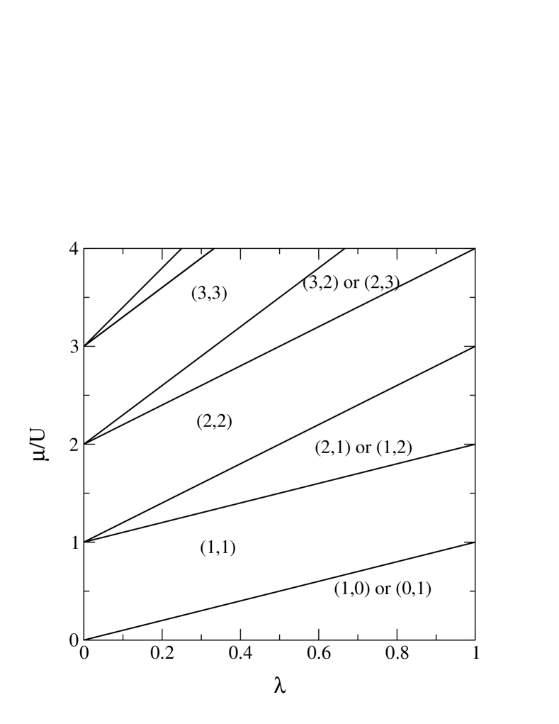
Figure 1: Schematic phase diagram of two-species boson model in the Mott insulating state for $t_{1}=t_{2}=0$. Notice the two-fold degeneracy at each site for odd fillings.

At finite hopping strengths, this degeneracy is lifted by quantum fluctuations which can be studied by second order perturbation theory. More precisely, one can carry out this perturbation theory in the regime $U,U^{\prime},|U-U^{\prime}|>>t_{1},t_{2}$ where we are far away from both the SU(2) symmetric limit ($\lambda=1$) and the vanishing inter-species interaction limit ($\lambda\ll 1$). In both these limits perturbation theory breaks down.

To compute the fluctuation correction for a Mott state with an odd number $n_{0}$ of atoms on each site, we divide the system into A and B sublattices (to allow for the possibility of an antiferromagnetic phase) and use a trial wave-function

$$\left|\Psi\right>=\prod_{i\in A}\prod_{j\in B}\left|\psi_{A}\right>_{i}\left|\psi_{B}\right>_{j}$$

where

$$\left|\psi_{A,B}\right>=\cos\frac{\theta_{A,B}}{2}\left|n_{0},n_{0}-1\right>+e^{i\phi_{A,B}}\sin\frac{\theta_{A,B}}{2}\left|n_{0}-1,n_{0}\right>$$

where $\left|n_{1},n_{2}\right>_{i}$ denotes $n_{1}$ and $n_{2}$ atoms of species $1$ and $2$ at site $i$. A perturbative calculation yields the ${\rm O}(t^{2}/U^{2})$ correction to the ground-state energy as a function of the angles $\theta_{A,B}$ and $\phi_{A,B}$:

$$E_{f} = -\frac{Nzt_{1}^{2}}{2U}\Bigg{[}(1+\eta^{2})n_{0}^{2}(1+\cos\theta_{A}\cos\theta_{B})$$ (4)

$$+(1-\eta^{2})n_{0}(\cos\theta_{A}+\cos\theta_{B})$$

$$+(1+\eta^{2})\left[1-\cos\theta_{A}\cos\theta_{B}\right]\left[\frac{n_{0}^{2}}{2\lambda}+\frac{n_{0}^{2}-1}{2-\lambda}\right]$$

$$+ \sin(\theta_{A})\sin(\theta_{B})\cos(\phi_{A}-\phi_{B})\frac{\eta n_{0}^{2}}{\lambda}\Bigg{]},$$

where $z$ is the coordination number of the lattice. Minimizing the

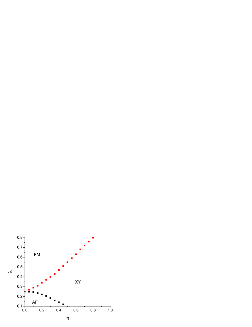
Figure 2: (Color online) Mean-field phase diagram of the effective low energy Hamiltonian in Eq. 4 obtained using perturbation theory at odd filling for $n_{0}=1$. The phase diagrams for other values of odd $n_{0}$ are qualitatively similar in the Mott insulating regime.

$E_{f}$ with respect to $\theta_{A,B}$ and $\phi_{A,B}$, we obtain the phase diagram shown in Fig. 2 for $n_{0}=1$ as a function of the parameters $\eta$ and $\lambda$. This phase diagram illustrates presence of three types of phases duan1 : a) antiferromagnetic (AF) phase with $\theta_{A(B)}=0,\theta_{B(A)}=\pi$, b) ferromagnetic (FM) phase with $\theta_{A}=\theta_{B}=0$, and c) XY phases with $\theta_{A}=\theta_{B}\neq 0$. The nature of the transitions between these effective isospin phases can be understood by plotting the values of the angles $\theta_{A}$ and $\theta_{B}$ across the different phase boundaries. These plots are shown in Fig. 3. Here the angles $\theta_{A}$ and $\theta_{B}$ have been plotted for three different values of $\eta$. In the XY and FM phases $\theta_{A}=\theta_{B}$ and the lines are indistinguishable, whereas in the AF phase one phase takes on a value $\pi$ and the other $0$. We find that there is always an abrupt jump from the XY to the AF phase across the AF phase boundary, suggesting that AF-XY transition is first order. We do not find any canted AF phases. The situation here is analogous to the first order melting transition of hard-core bosons with next nearest-neighbor interaction at half filling bs . The FM-XY transition, on the other hand, is continuous and proceeds via continuous change of $\theta_{A}$ and $\theta_{B}$.

The phase diagram obtained here agrees qualitatively with that of Ref. duan1, , although there is a quantitative difference. In our phase diagram, the tricritical point where all the phases meet is at $\lambda=0.25,\eta=0$ instead of $\lambda=0.5,\eta=0$, as found in Ref. duan1, . To understand why this difference arises, we now map the boson Hamiltonian to an effective low-energy spin-model. Defining the isospin operators $S^{z}_{i}=(n_{1i}-n_{2i})/2$, $S^{x}_{i}=(b_{1i}^{\dagger}b_{2i}+b_{2i}^{\dagger}b_{1i})/2$ and $S^{y}_{i}=i(b_{1i}^{\dagger}b_{2i}-b_{2i}^{\dagger}b_{2i})/2$ one obtains an effective XXZ model in a magnetic field demler1 ; duan1

$${\mathcal{H}}_{\rm XXZ} = -\sum_{\left<ij\right>}\Big{[}J_{\perp}\left(S^{x}_{i}S^{x}_{j}+S^{y}_{i}S^{y}_{j}\right)+J_{z}S^{z}_{i}S^{z}_{j}\Big{]}$$ (5)

$$-B\sum_{i}S^{z}_{i}+U(1-\lambda)\sum_{i}S_{zi}^{2}.$$

The exchange couplings $J_{\perp},J_{z}$ and the magnetic field $B$ are given by

$$J_{\perp} = \frac{4t_{1}^{2}\eta n_{0}^{2}}{\lambda U},\quad\quad B=\frac{2zt_{1}^{2}(1-\eta^{2})n_{0}}{U},$$

$$J_{z} = \frac{4t_{1}^{2}}{U}(1+\eta^{2})\left[n_{0}^{2}\left(1-\frac{1}{2\lambda}\right)-\frac{n_{0}^{2}-1}{2-\lambda}\right].$$ (6)

Note that for $n_{0}=1$, AF, FM and XY phases meet when $J_{z}=J_{\perp}=0$ at $\lambda=0.5,\eta=0$ provided one neglects the magnetic field term, as done in Ref. duan1, . However, if one retains the magnetic field term, the AF and the FM phases will meet when $J_{z}+2B/z=0$ and $J_{\perp}=0$ or $\lambda=0.25,\eta=0$.

The XY phase obtained here is identical to the superfluid counterflow (SCF) phase obtained in Ref. kuklov1, and also to the $\nu=1$ bilayer quantum Hall state for small layer separation where the layer index plays the role of isospin steve1 ; steve2 . The stiffness energy locking the two order parameter phases together in the XY phases can be obtained from Eq. 4

$$\rho_{s} = \left(\frac{\partial^{2}E_{f}}{\partial(\phi_{A}-\phi_{B})^{2}}\right)_{\phi_{A}=\phi_{B}}=\frac{Nzt_{1}^{2}\eta n_{0}^{2}}{2U\lambda}\sin{\theta_{A}}\sin{\theta_{B}}$$

Note that the $U(1-\lambda)\sum_{i}S_{zi}^{2}$ term in ${\mathcal{H}}_{\rm XXZ}$ is a constant since $S_{zi}^{2}=1/4$ for all the states in the low energy manifold with $S_{zi}=\pm 1/2$. Hence this term does not contribute to the low energy effective Hamiltonian and does not play a role in the quantum disordering of the XY phase. The disordering of the XY phase due to quantum fluctuation depends only on the exchange constants $J_{z},J_{\parallel}$ and $B$.

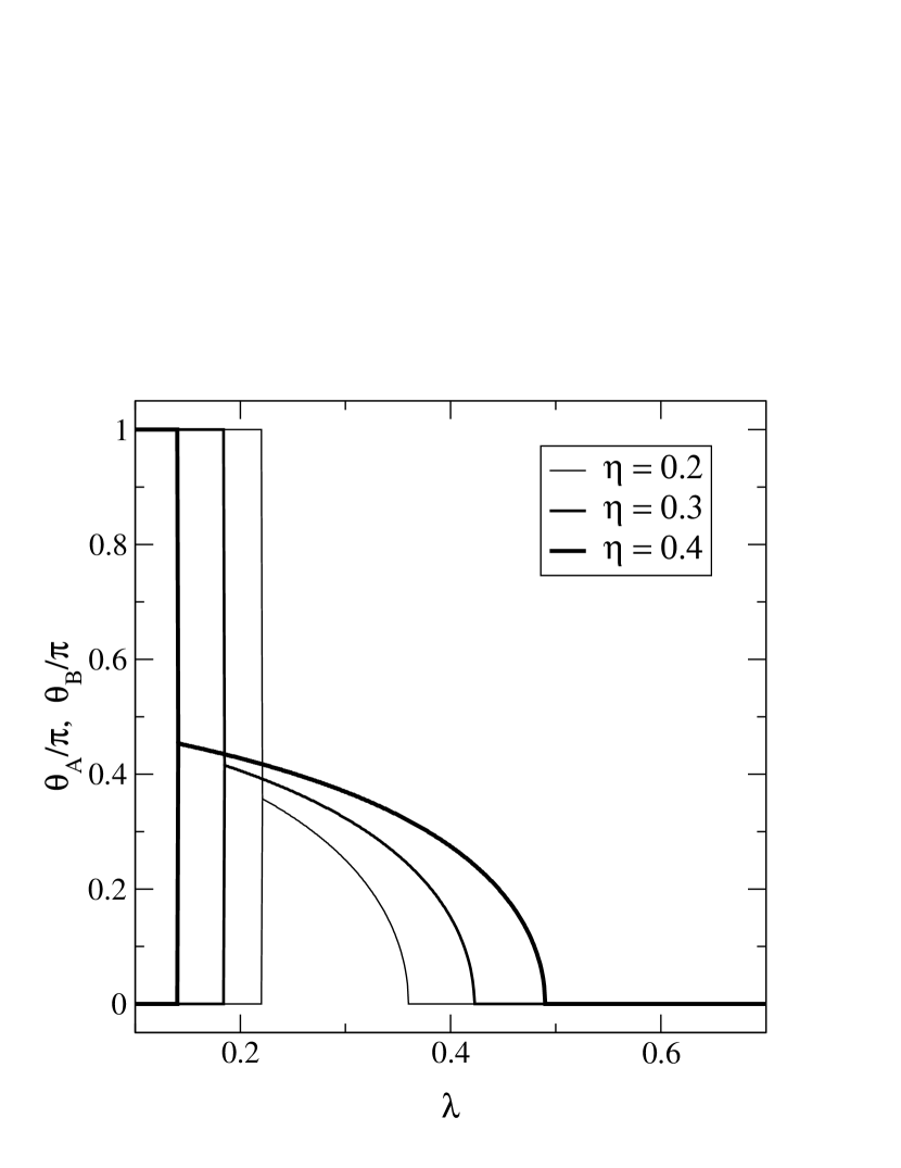
Figure 3: Plot of optimum values of $\theta_{A}$ and $\theta_{B}$ as a function of $\lambda$ for different values of $\eta$. In the XY and FM phases $\theta_{A}=\theta_{B}$ and the lines for $\theta_{A(B)}$ are indistinguishable whereas in the AF phase one angle takes on a value $\pi$ while the other takes on a zero value. We find a discontinuous change in both $\theta_{A}$ and $\theta_{B}$ as the AFM phase is entered, signaling a first-order transition.

III ${\rm O}(t/U)$ Mean-field theory for the SI transition

In this section, we shall study the SI transition within ${\rm O}(t/U)$ mean-field theory by constructing a site factorizable variational wavefunction which provides an analytical albeit qualitative understanding of the transition. We shall work in the parameter regime where $U,U^{\prime},|U-U^{\prime}|\gg t_{1},t_{2}$. For the sake of clarity, although we shall qualitatively comment on the general case, all calculations in this section from here on shall be performed for two spatial dimensions and $n_{0}=1$.

Before carrying out the mean-field analysis, we review earlier studies of SI transition for the two species Bose-Hubbard model (Eq. 2). In Ref. chen1, , the SI transition has been studied for the case $t_{1}=t_{2}$ but with different inter-species and intra-species interaction strengths and chemical potentials. This has been done using a standard mean-field theory Sachdev1 corresponding to decoupling the hopping between sites by introducing order parameter fields $\Delta_{\alpha}$, i.e. $b^{\dagger}_{i\alpha}b_{j\alpha}\approx b^{\dagger}_{i\alpha}\Delta_{\alpha}+b_{j\alpha}\Delta_{\alpha}^{*}-|\Delta_{\alpha}|^{2}$ where the fields $\Delta_{\alpha}$ satisfy the self consistency relations $\Delta_{\alpha}=\left<b_{\alpha}\right>$. Their analysis led to the prediction of three different phases (1) Both species superfluid (SF-SF). (2) Species 1 superfluid and species 2 in a Mott state (SF-MI). (3) Species 2 superfluid and species 1 in a Mott state. (MI-SF). It has been found (erroneously, as we shall see) in Ref. chen1, that the Mott states are always destabilized by MI-SF or SF-MI phases and there is no direct transition from the Mott to the SF-SF phase. The transitions are concluded to be second order as in the standard single species Bose-Hubbard model Sachdev1 . The question of the interplay between the exchange effects and the SI transition in the region of small $\lambda$ was studied by Demler et al. demler1 for unit filling factor and fixed chemical potential $\mu/U=\frac{1}{2}\lambda$. Apart from the phases mentioned above they also found a superfluid phase with species one superfluid and depopulation of species $2$.

In our proposed setup, $\lambda$ is not necessarily small and the SI transition in this regime has not previously been investigated. To analyze the SI transition to ${\rm O}(t/U)$ within mean field it suffices to consider an on-site trial wavefunction comment1

$$\left|\Psi_{v}\right> = \prod_{i}\Bigg{(}u_{0}\left|1,0\right>_{i}+r\left|0,1\right>_{i}+p_{1}\left|2,0\right>_{i}$$ (7)

$$+p_{2}\left|1,1\right>_{i}+p_{3}\left|0,2\right>_{i}+h_{1}\left|0,0\right>_{i}\Bigg{)}$$

where $u_{0}$ is the amplitude of the ferromagnetic Mott state $\left|1,0\right>$ in $\Psi_{v}$, $h$ and $p$ are amplitudes of removing, adding bosons of species $1,2$ to the Mott state and $r$ is the amplitude of isospin-flip. We note here that allowing the isospin-flip process in the trial wavefunction (Eq. 7) is absolutely crucial for correctly taking into account the manifold of low energy boson states which are degenerate to ${\rm O}(t/U)$. The normalization of the wave-function yields the constraint $u_{0}^{2}+r^{2}+p_{1}^{2}+p_{2}^{2}+p_{3}^{2}+h_{1}^{2}=1$. This wavefunction, as we shall see, is appropriate for studying the SI transition from the FM and the XY Mott phases. We shall comment about the AFM-SI transition later.

The energy of the variational ground state $E_{v}(u_{0},r,p_{1},h_{1},p_{2},h_{2})=\left<\Psi_{v}\right|{\mathcal{H}}\left|\Psi_{v}\right>$ is given by

$$E_{v} = E_{Mott}+\Bigg{[}(p_{1}^{2}+p_{3}^{2})\delta E_{1}^{+}+p_{2}^{2}\delta E_{2}^{+}+h_{1}^{2}\delta E_{1}^{-}$$ (8)

$$-\sum_{\alpha=1,2}\frac{\Delta_{\alpha}^{2}}{zt_{\alpha}}\Bigg{]},$$

where $E_{Mott}$ is the energy of the Mott state, $z$ is the coordination number of the lattice, $\delta E_{\alpha}^{\pm}$ denote the energies of adding/removing a boson of species $\alpha$ to/from the Mott state given by

$$\delta E_{1}^{+} = -\mu+U,\quad\delta E_{2}^{+}=-\mu+\lambda U\quad\delta E_{1}^{-}=\mu,$$ (9)

and the superfluid order parameters $\Delta_{1,2}$ can be calculated from this variational wave-function:

$$\Delta_{1} = zt_{1}\left<\Psi_{v}\right|b_{1}\left|\Psi_{v}\right>=zt_{1}\left(u_{0}p_{1}\sqrt{2}+rp_{2}+u_{0}h_{1}\right)$$

$$\Delta_{2} = zt_{2}\left<\Psi_{v}\right|b_{2}\left|\Psi_{v}\right>=zt_{2}\left(u_{0}p_{2}+rh_{1}+rp_{3}\sqrt{2}\right)$$ (10)

Mathematically, it is possible to show that for all of the Mott and superfluid phases (except the AFM phase for which we need to use two sublattices), the variational energy has a stationary point. The parameter values at these points and how they translate into the various phases is shown in Table 1.

Phase	$u_{0}$	$r$	$p_{1}$	$p_{2}$	$p_{3}$	$h_{1}$
FM Mott-Insulator	1	0	0	0	0	0
XY Mott-Insulator	$\neq 0$	$\neq 0$	0	0	0	0
SF1,MI2	0	$\neq 0$	0	$\neq 0$	0	0
MI1, SF2	$\neq 0$	0	0	$\neq 0$	0	0
SF1, 02 (a-SF)	$\neq 0$	0	$\neq 0$	0	0	$\neq 0$
SF1,SF2	$\neq 0$	$\neq 0$	$\neq 0$	$\neq 0$	$\neq 0$	$\neq 0$

Table 1: Parameter values of the variational wavefunction corresponding to the different phases.

The transition to superfluidity from the Mott state occurs when it becomes energetically favorable to have non-zero $\Delta_{\alpha}$ ${\it i.e.}$ non-zero amplitudes of additional particles and holes ($p$ and $h$) in the variational ground state. For our purposes, it is sufficient to take all the coefficients real. This amounts to setting the phase of the superfluid order parameter to zero and does not affect the variational energy of the state. Note that the wavefunction (Eq. 7) is general enough to incorporate both the FM ($u_{0}=1$) and the XY ($u_{0}=\cos(\theta/2)$ $r=\sin(\theta/2)$) phases of the Mott state. However, since these two states are degenerate to ${\rm O}(t/U)$, our simple mean-field treatment cannot distinguish between their isospin order. In Secs. IV and V we shall carry out more sophisticated treatments of our model which will take into account the effect of ${\rm O}(t^{2}/U^{2})$ fluctuations using canonical transformation and quantum Monte-Carlo. In this section, we shall analyze the ${\rm O}(t/U)$ mean-field theory and point out certain qualitative features of the phase diagram.

III.1 General features of the phase diagram

Although the variational wave function in this section excludes second order exchange effects, the qualitative features of the SI transition from the FM and the XY phases for $n_{0}=1$ can be understood from Eqs. 8 and 9. Consider, for example, approaching the SI transition from FM/XY Mott phase. For $\mu\ll U,\lambda U$, since $\delta E_{1}^{-}\ll\delta E_{1}^{+},\delta E_{2}^{+}$, at the SI transition point $t_{1}\equiv t_{1}^{c}=\delta E_{1}^{-}/z$ and the energy of the variational wavefunction is minimized with $r=0$, $u_{0}\sim 1$, $p_{1}=p_{2}=p_{3}=0$, $h_{1}\neq 0$. Consequently, from Eq. 10, we have $\Delta_{2}=0$, $\Delta_{1}\neq 0$, and also

$$n_{1} = \left<\Psi_{v}\right|b_{1i}^{\dagger}b_{1i}\left|\Psi_{v}\right>=\left(u_{0}^{2}+2p_{1}^{2}+p_{2}^{2}\right)\equiv 1$$

$$n_{2} = \left<\Psi_{v}\right|b_{2i}^{\dagger}b_{2i}\left|\Psi_{v}\right>=\left(r^{2}+2p_{3}^{2}+p_{2}^{2}\right)=0$$ (11)

Thus the transition to superfluidity occurs with complete depopulation of species $2$. We refer to this phase as a-SF. Alternatively one can view this phase as SF₁-MI₂ with a zero filling factor in the Mott phase. Numerically, we find that such a depopulation occurs till a critical value of $\mu=\mu_{c1}$.

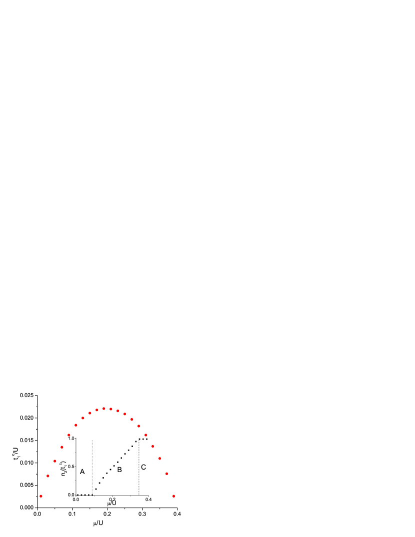
Figure 4: (Color online) ${\rm O}(t/U)$ mean-field results for the SI transition from the XY phase for $\lambda=0.4$ and $\eta=0.8$. The inset shows $n_{2}$ at the transition. Superfluidity sets in a) with depopulation bosons of species $2$ in region A (a-SF phase) b) simultaneously for both species in region B (SF-SF) and c) with Mott phase for $2$ and superfluid for $1$ in region C (${\rm MI}_{2}+{\rm SF}_{1}$). The vertical dotted lines are guides to the eye and represent the positions of $\mu_{c1}$ and $\mu_{c2}$ (see text).

In the other limit, when $\mu\simeq\lambda U\geq\mu_{c2}$, it is much more favorable to destabilize the Mott state by adding a particle of species 2 since $\delta E_{2}^{+}\ll\delta E_{1}^{-},\delta E_{1}^{+}$. As a result the transition occurs with $u_{0}=0$, $r\simeq 1$ and $p_{2}\neq 0$. Consequently, the transition takes place with

$$\Delta_{2} = 0,\quad n_{2},\,\,\Delta_{1},\,\,n_{1}\neq 0$$ (12)

$i.e.$, we have a transition which is accompanied by a jump of population species $2$ at the transition. The phase consists of a Mott insulator of species $2$ (since $\Delta_{2}=0$) and superfluid of species $1$. We call this state ${\rm MI}_{2}+{\rm SF}_{1}$.

For $\mu_{c2}>\mu>\mu_{c1}$, $\delta E_{2}^{+}$ and $\delta E_{1}^{-}$ are comparable and the energy of the ground state at the transition is minimized for $r,u_{0}\neq 0$ and $p_{2}\neq 0$. In this case, provided $\eta\neq 0$, both $\Delta_{1}$ and $\Delta_{2}$ are non-zero at the transition implying simultaneous onset of superfluidity of species $1$ and $2$ (referred to as SF-SF). The width of this region is expected to be large at large $\eta$, since higher $t_{2}$ makes it energetically more favorable to realize superfluidity of species $2$.

The values of $\mu_{c1}$ and $\mu_{c2}$ are shown for representative values of $\eta=0.8$ and $\lambda=0.4$ in Fig. 4. The phase diagram corroborates the above discussion. From the inset of Fig. 4, we find that there are three distinct regions where the SI transition takes place with a) depopulation of species $2$ (region A), b) simultaneous setting of superfluidity of the two species (region B), and c) Mott insulating phase of species $2$ and superfluidiy of species $1$ (region C). The situation here is in sharp contrast to the even filling case which will always have an intermediate state with superfluidity of species $1$ and insulating state of species $2$ for $0<\eta<1$.

Upon further increase of $t_{1}$ from the critical value $t_{1c}$, two scenarios are possible. If superfluidity sets in with depopulation, increasing $t_{1}$ does not change the situation further. On the other hand, if the transition occurs to either the SF-SF or ${\rm MI}_{2}+{\rm SF}_{1}$ phase, upon increasing $t_{1}$, the fraction of B atoms in the superfluid decreases as shown in Fig. 5 for a set of representative values of $\eta$, $\lambda$ and $\mu$. Finally, one crosses a critical value $t_{1}^{\ast}$ at which it becomes energetically favorable for the system to depopulate. This happens at large enough $t_{1}\geq t_{1}^{\ast}\sim\delta E_{1}^{+}/z$, at which the variational energy minima shifts to $u_{0}\neq 0$, $r=p_{2}=0$. Beyond this point, we only find superfluidity of species $1$. Within ${\rm O}(t/U)$ mean-field theory, such a transition from SF-SF to a-SF phase is found to be first order since $\sum_{\alpha=1,2}\Delta_{\alpha}^{2}/zt_{\alpha}$ is discontinuous across the transition.

Although we do not show it explicitly here, a similar consideration remains valid for the SI transition from the AFM phase. This can again be seen by dividing the lattice into the usual $A$ and $B$ sublattices and constructing an appropriate two sublattice variational wavefunction. We do not find any translational symmetry broken superfluid phases. We also note that the above discussions have to be modified for $n_{0}\neq 1$, where the Mott state can also be destabilized by adding holes of species $2$. For example, when $n_{0}\gg 1$, for $\mu\ll\lambda$, $\delta E_{1}^{-}\approx\delta E_{2}^{-}$. Thus if $\eta\neq 0$, we expect the ground state energy to be always minimized for $u_{0},r\neq 0$ at the transition. Consequently, there will be no depopulation for any finite $\eta$ in this limit. In the rest of this work, we shall restrict all discussion to odd fillings with $n_{0}=1$.

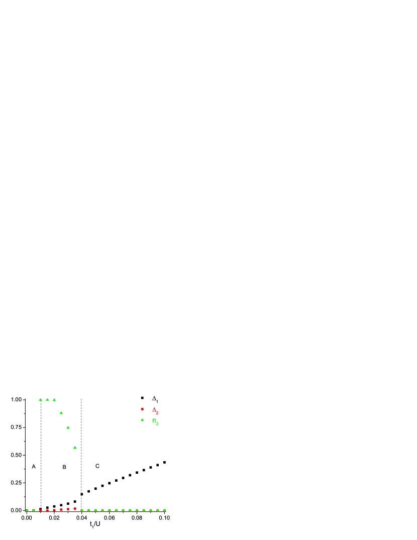
Figure 5: (Color online) A plot of the order parameters $\Delta_{1}$, $\Delta_{2}$, and $n_{2}$ for $\mu/U=0.57$, $\lambda=0.6$ and $\eta=0.2$ as a function of the hopping amplitude $t_{1}$. The system enters the ${\rm MI}_{2}+{\rm SF}_{1}$ phase at $t=t_{1}^{c}$ (vertical dotted line between regions A and B) from a FM Mott phase (region A). Note that the transition occurs with a spontaneous jump of $n_{2}$ and is hence expected to be first order. As we increase $t_{1}$, both species becomes superfluid (region B), until $t_{1}$ reaches $t_{1}^{\ast}$ (vertical dotted line between region B and C) where the system depopulates. The depopulation occurs with a jump in $\Delta_{1}$ and is therefore first order.

III.2 Necessity of going beyond the ${\rm O}(t/U)$ mean-field theory

We now discuss the limitations of the mean-field theory to set the stage for incorporating the fluctuation effects. To understand why using the mean-field theory is dangerous in the present context, consider plotting the mean-field phase diagram at a fixed $\mu/U=0.5$ and $t_{1}/U=0.04$ as a function of $\eta$ and $\lambda$. Such a phase diagram is shown in Fig. 6. Here, we have used the phase diagram (Fig. 2) of the XXZ model [Eq. (5)] to determine the isospin phases since the ${\rm O}(t/U)$ mean-field theory can not distinguish between them. As can be seen, the phase diagram (Fig. 6) corroborates the expectations based on the qualitative discussion of the Sec. III.1. For small $\eta$ (transition from FM/AFM phases), the system favors a-SF phase while for larger $\eta$ (transition from the XY-phase) the SF-SF phase dominates.

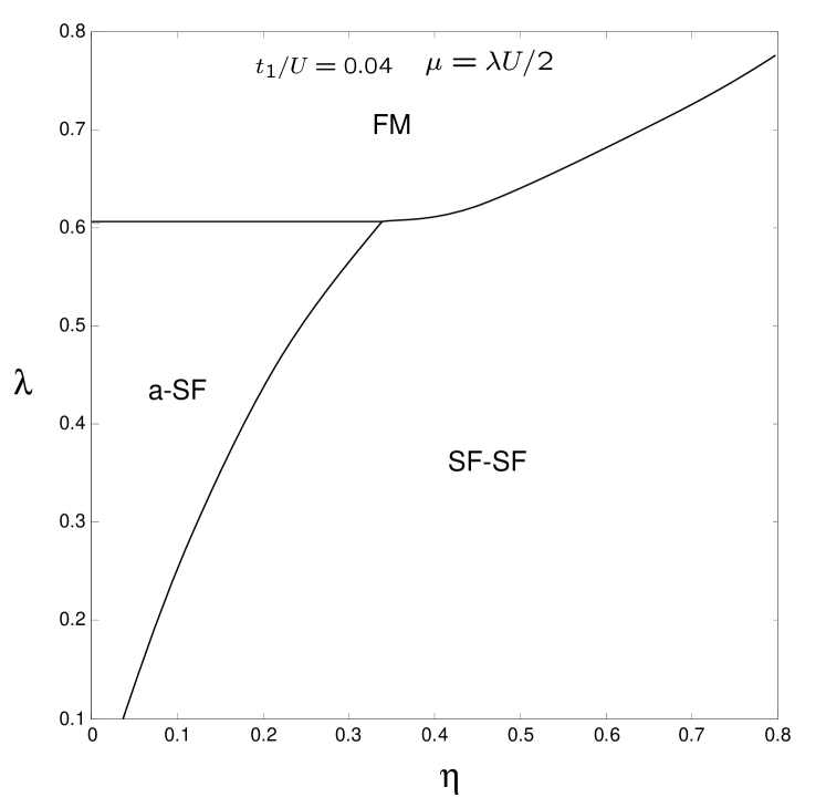
Figure 6: ${\rm O}(t/U)$ mean-field phase diagram for the two-species model as a function $\eta$ and $\lambda$ for $\mu/U=\lambda/2$ and $t_{1}/U=0.04$. In the absence of second order fluctuation corrections, the SF-SF phase borders to the FM phase implying a discontinuous change in the population of species 2 for a large region of parameter phase.

However, consider now plotting such a phase diagram near $\mu_{c1}$ or $\mu_{c2}$. Clearly, we expect that incorporating exchange effects will make it harder for the isospins to flip, since now it costs an energy ${\rm O}(t^{2}/U^{2})$. This will, in general, shift the positions of $\mu_{c1}$ and $\mu_{c2}$ from their mean-field values. Therefore, near $\mu_{c1}$ or $\mu_{c2}$, the phase diagrams in the $\eta-\lambda$ plane predicted by the mean-field theory will be qualitatively different from the true phase diagrams. In this sense, the failure of the ${\rm O}(t/U)$ mean-field theory in the present case is much more severe compared to the usual SI transition for single species bosons. However, as long as we are away form the critical $\mu$ values, such a mean-field theory gives qualitatively correct results and therefore the scenario described in the previous section remains largely valid.

Another problem of the ${\rm O}(t/U)$ mean-field theory is that it overestimates the jump of $n_{1}$ or $n_{2}$ at the transition since it does not take into account the energy cost of an isospin flip. Consequently, it can erroneously predict first-order MI-SF or a-SF to SF-SF transitions where in reality such transitions might be second order. Also, as we shall see in the next section, the shapes of the transition curves and topology of phase boundaries change quite a bit upon inclusion of the fluctuation corrections.

Thus, although the ${\rm O}(t/U)$ mean-field theory correctly predicts the qualitative nature of the MI-SF transition for most parts of the phase diagram it fails drastically either when we are close to $\mu_{c1}$ or $\mu_{c2}$ or when we want to estimate the order of the transition. In the next section, we remedy this failure by incorporating the ${\rm O}(t^{2}/U^{2})$ fluctuation corrections.

IV Canonical Transformation

The effect of fluctuation to second order in $t/U$ can be taken into account using a suitable canonical transformation method. We describe the implementation of this method in subsection  IV.1 and present the phase diagrams in subsection IV.2.

IV.1 Implementing the canonical transformation

We begin by separating the Bose-Hubbard Hamiltonian (Eq. 2) into an onsite term $H_{0}=\sum_{i}H_{i}$ (Eq. LABEL:onsite) and the hopping terms $T$. The first step is to write $T$ in terms of sum over bonds $\sigma$ between the neighboring lattice site. To this end, as shown in Fig. 7, we can decompose the hopping into hopping on vertical and horizontal bonds, labeled $\sigma_{v,h}$, between adjacent sites. The hopping term can then be written as a sum over bonds

$$T = \sum_{\sigma}T_{\sigma}=\sum_{\sigma_{h}}T_{\sigma_{h}}+\sum_{\sigma_{v}}T_{\sigma_{v}}$$ (13)

$$T_{\sigma_{h}} = -\sum_{\alpha}t_{\alpha}\left(b_{\sigma_{h_{R}}\alpha}^{\dagger}b_{\sigma_{h_{L}}\alpha}+{\rm h.c}\right)$$ (14)

$$T_{\sigma_{v}} = -\sum_{\alpha}t_{\alpha}\left(b_{\sigma_{v_{U}}\alpha}^{\dagger}b_{\sigma_{v_{D}}\alpha}+{\rm h.c}\right)$$ (15)

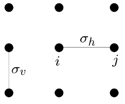
Figure 7: Bonds in a 2D square lattice. There are two types of bonds, horizontal and vertical labeled by $\sigma_{h}$ and $\sigma_{v}$ respectively. The horizontal bond shown is denoted by $\sigma_{h}$. The sites on the left and right sides of this bond of (sites $i$ and $j$ in this case) are labeled by $\sigma_{h_{L}}$ and $\sigma_{h_{R}}$ respectively.

We now seek a unitary transformation that will capture the effects of the second order exchange effects. We shall only consider the case $n_{0}=1$, although generalization to other values of $n_{0}$ is straightforward. To do this, we first introduce the projection operators $P_{\sigma}$ acting on the two sites associated with each bond $\sigma$. $P_{\sigma}$ projects the state of the system to the manifold of states having one particle on each site of the bond. Such a projection operator can be decomposed into two parts depending on whether the bosons occupying the sites of the bond are of the same or different species: $P_{\sigma}=P_{\sigma}^{0}+P_{\sigma}^{1}$. For instance for a horizontal bond we can write

$$P_{\sigma_{h}} = P_{\sigma_{h}}^{0}+P_{\sigma_{h}}^{1}$$

$$P_{\sigma_{h}}^{0} = \left(\left|1,0\right>\left<1,0\right|\right)_{\sigma_{h_{L}}}\otimes\left(\left|1,0\right>\left<1,0\right|\right)_{\sigma_{h_{R}}}$$ (16)

$$+\left(\left|0,1\right>\left<0,1\right|\right)_{\sigma_{h_{L}}}\otimes\left(\left|0,1\right>\left<0,1\right|\right)_{\sigma_{h_{R}}}$$

$$P_{\sigma_{h}}^{1} = \left(\left|0,1\right>\left<0,1\right|\right)_{\sigma_{h_{L}}}\otimes\left(\left|1,0\right>\left<1,0\right|\right)_{\sigma_{h_{R}}}$$ (17)

$$+\left(\left|1,0\right>\left<1,0\right|\right)_{\sigma_{h_{L}}}\otimes\left(\left|0,1\right>\left<0,1\right|\right)_{\sigma_{h_{R}}}$$

where the state $\left|1,0\right>$ denotes $\left|n_{1}=1,n_{2}=0\right>$ as before and the subscript on the parentheses denotes the bond and which of the sites the operators act on (cf. Fig. 7). Using the projection operator (Eqs. 16,17), we now decompose $T_{\sigma}$ (Eq. 13) into two parts

$$T_{\sigma} = P_{\sigma}^{\bot}T_{\sigma}P_{\sigma}^{\bot}+\left(T_{\sigma}P_{\sigma}+P_{\sigma}T_{\sigma}\right)=T_{\sigma}^{0}+T_{\sigma}^{1}$$ (18)

where $P_{\sigma}^{\bot}=1-P_{\sigma}$. The idea is now to use these results to seek a unitary transformation

$$H^{*} = e^{iS}{\mathcal{H}}e^{-iS}={\mathcal{H}}+[iS,{\mathcal{H}}]+\frac{1}{2}\left[iS,\left[iS,{\mathcal{H}}\right]\right]+...$$

which eliminates the terms $T_{\sigma}^{1}$ to ${\rm O}(t/U)$. It turns out that a suitable choice of $S$ is

$$S = \frac{i}{\lambda U}\sum_{\sigma}[\lambda P_{\sigma}^{0}+P_{\sigma}^{1},T_{\sigma}]=\frac{i}{\lambda U}\sum_{\sigma}[P_{\sigma}^{\lambda},T_{\sigma}]$$ (20)

where we have introduced the notation $P_{\sigma}^{\lambda}=\lambda P_{\sigma}^{0}+P_{\sigma}^{1}$ for future convenience. We now expand $H$ (Eq. LABEL:trans) in powers of $S$. Since $S$ is first order in $t/U$, this is equivalent to an expansion in $t/U$ and we have to ${\rm O}(t^{2}/U^{2})$,

$$H^{*} = H_{0}+\sum_{\sigma}T_{\sigma}+\left[iS,H_{0}+\sum_{\sigma}T_{\sigma}\right]$$ (21)

$$+\frac{1}{2}\left[iS,\left[iS,H_{0}\right]\right]+{\rm O}(t^{3}/U^{3})$$

We now evaluate the different terms in Eq. (21). The algebra is straightforward, but lengthy and we present some details in Appendix A. The final result, to ${\rm O}(t^{2}/U^{2})$, is

$$H^{*} = H_{0}+\sum_{\sigma}P_{\sigma}^{\bot}T_{\sigma}P_{\sigma}^{\bot}$$

$$-\frac{1}{2\lambda U}\sum_{\sigma}\left[P_{\sigma}^{\lambda}T_{\sigma}^{2}P_{\sigma}-T_{\sigma}P_{\sigma}^{\lambda}T_{\sigma}+{\rm h.c.}\right]$$

$$-\frac{1}{\lambda U}\sum_{\sigma,j}\left[P_{\sigma}^{\lambda}T_{\sigma}T_{\sigma+j}-T_{\sigma}P_{\sigma}^{\lambda}T_{\sigma+j}\right.$$

$$\left.-2\left(P_{\sigma}^{\lambda}T_{\sigma}T_{\sigma+j}P_{\sigma+j}-T_{\sigma}P_{\sigma}^{\lambda}P_{\sigma+j}T_{\sigma+j}\right)+{\rm h.c.}\right]$$

where the sum over $j$ extends over bonds which are nearest neighbors to $\sigma$. We note that the third and the fourth terms of Eq. LABEL:hamf represent the effective XXZ model [Eq. (5)] of Section II and the two-particle hopping processes respectively, whereas the terms in the last line involve hopping operators on neighboring bonds and are expected to be important in the superfluid phases.

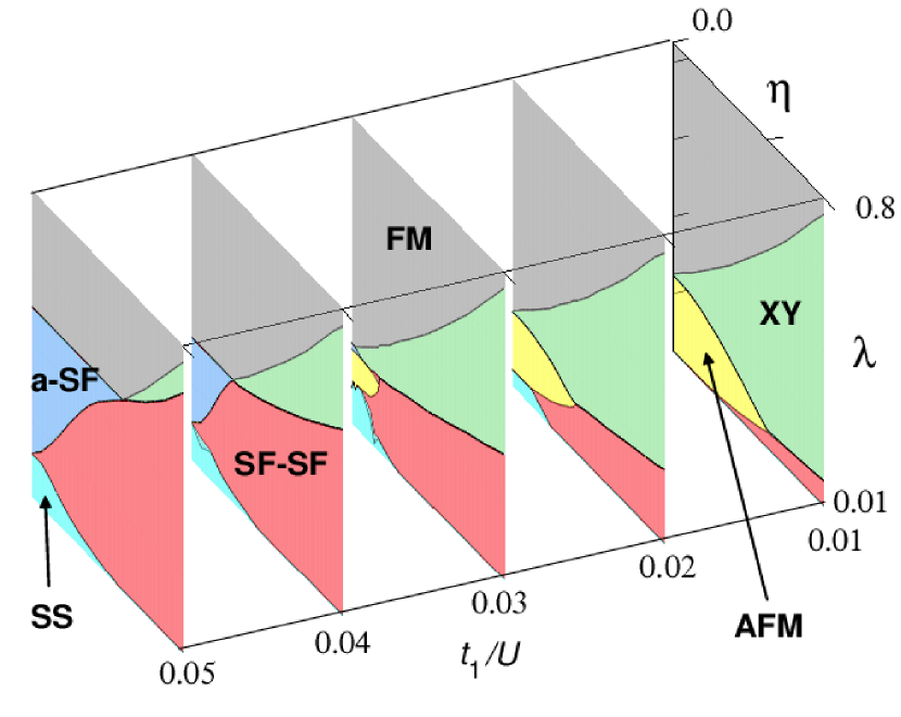
Figure 8: (Color online) ${\rm O}(t^{2}/U^{2})$ mean-field phase diagram for the two-species model as a function $\eta$ and $\lambda$ for $\mu=\lambda U/2$. The plot for $t_{1}/U=0.04$ should be compared with the phase diagram obtained to ${\rm O}(t/U)$ in Fig. 6 (see text). Note the gradual evolution of the different phases with increase of $t_{1}$. The existence of the multicritical point is due to the special symmetry at $\mu=\lambda U/2$ where adding a hole or a particle of species 2 to the FM Mott state cost equal energies. Quantum Monte Carlo however reveals that these multicritical points can be split (See Sec. V).

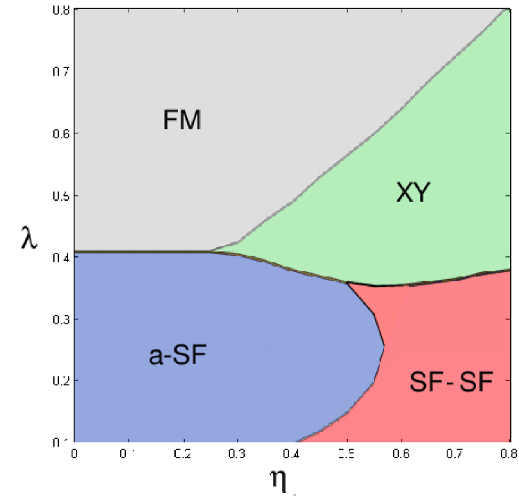
Figure 9: (Color online) ${\rm O}(t^{2}/U^{2})$ mean-field phase diagram for the two-species model as a function $\eta$ and $\lambda$ for $\mu/U=0.1\lambda$ and $t_{1}/U=0.01$. The superfluidity is a-SF for a large parameter regime as predicted by the ${\rm O}(t/U)$ mean-field theory.

IV.2 Phase Diagram

The phase diagram of $H^{\ast}$ is obtained by dividing the lattice into two sublattices $A$ and $B$ and using an on-site variational wavefunction $\left|\psi_{v}\right>=\prod_{i\in A}\prod_{j\in B}\left|\psi\right>_{i}\left|\psi\right>_{j}$. The division into two sublattices is essential for taking into account the AFM phase. We note that this is equivalent to generalizing the mean-field treatment of Sec. III to incorporate second order fluctuation corrections. Although it is cumbersome to evaluate the expectation value $\left<\psi_{v}\right|H^{\ast}\left|\psi_{v}\right>$ analytically, it can be calculated numerically by representing the various operators in the Hamiltonian as matrices in an appropriately chosen basis. The task of minimizing $\left<\psi_{v}\right|H^{\ast}\left|\psi_{v}\right>$ is then a numerical optimization problem. Truncating the Hilbert space to have at most two particles on each site, we perform constrained (to keep the norm to unity) optimization for each point in the phase diagram. We use a sequential quadratic programming algorithm from the MATLAB (TM) optimization toolbox for this task. Due to nontrivial energy landscapes and possible existence of first order transitions, several starting points,including random starting points, were used as input to the algorithm.

First, we show the phase diagram in the $\eta-\lambda$ plane for $\mu/U=0.5\lambda$ in Fig. 8, which shows the gradual evolution of the phases of the system as $t_{1}$ is increased. A comparison of Fig. 8 for $t_{1}/U=0.04$ to its ${\rm O}(t/U)$ mean-field counterpart [Fig. (6)], immediately shows us the importance of incorporating the exchange effects. Whereas the ${\rm O}(t/U)$ mean-field phase diagram shows a large boundary between the FM and the SF-SF phase indicating a first order transition, Fig 8 shows only second order phase boundaries and no direct transition between FM and SF-SF phases. This clearly points out that incorporating the exchange effects can lead to qualitatively different results.

The transition between the FM and the a-SF phases is second order, as expected. The transition between the a-SF and SF-SF phases is also found to be second order, in contrast to the prediction of the ${\rm O}(t/U)$ mean-field theory. This is a consequence of incorporating the second order fluctuation corrections. We note that the a-SF - SF-SF transition can alternatively be viewed as a Mott-insulator (with $n_{0}=0$) - superfluid transition of species $2$ in the presence of species $1$ in a superfluid state. The supersolid (SS) phase obtained for small values of $\lambda$ and $\eta$ represents a superfluid phase with broken sublattice symmetry. This is precisely the region where $zt^{2}/\lambda U$ becomes large and the perturbation theory breaks down. We shall see in the next section using Monte Carlo that the SS phase is indeed an artifact and signifies the breakdown of perturbation theory.

Similar phase diagrams for $\mu/U=0.1\lambda$ and $\mu/U=0.9\lambda$ and $t_{1}/U=0.01$ are shown in Figs. 9 and 10 respectively. These plots confirm that the qualitative expectations of the ${\rm O}(t/U)$ mean-field theory. For $\mu/U=0.1\lambda$, we find a large a-SF region and the transition to a-SF occurs from both FM and XY phases [Fig. (9)], the transitions from XY to a-SF being first order. For $\mu/U=0.9\lambda$ (Fig. 10), the a-SF phase is replaced by ${\rm MI}_{2}+{\rm SF}_{1}$. Here we find a direct first order transition between the FM and ${\rm MI}_{2}+{\rm SF}_{1}$ phases. These first order transitions are in perfect agreement with the predictions of the ${\rm O}(t/U)$ mean-field theory.

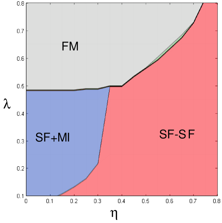
Figure 10: (Color online) ${\rm O}(t^{2}/U^{2})$ phase diagram for the two-species model as a function $\eta$ and $\lambda$ for $\mu/U=0.9\lambda$ for $t_{1}/U=0.02$. We see a large area of ${\rm MI}_{2}+{\rm SF}_{1}$ phase again in accordance with the mean-field theory prediction.

V Quantum Monte Carlo

To verify that the inclusion of ${\rm O}(t^{2}/U^{2})$ corrections using the canonical transformation procedure as carried out in section IV really gives an improvement over the ${\rm O}(t/U)$ mean-field theory in section III, we have performed quantum Monte Carlo (QMC) studies using the Stochastic Series Expansion method introduced by Sandwik ${\it et\,al.}$ Sandwik1 ; Sandwik2 . Here we have used a particular form of these updates, directed loop-updates. For details see Ref. Syljuasen, . The basis states used were from a truncated Hilbert space in which each site hosts at most two atoms per site, in the same way as done in the mean-field and canonical transformation treatments. We expect such a truncation to be adequate for reproducing the phase diagram since we work with $n_{0}=1$ and are always close to the MI-SF transition. We have investigated phase diagrams in the range $\mu/U=0.1\lambda-0.8\lambda$ and found Monte-Carlo results agreeing well with the qualitative predictions of both Secs. III and IV and we now turn to a critical comparison between the results obtained by different methods.

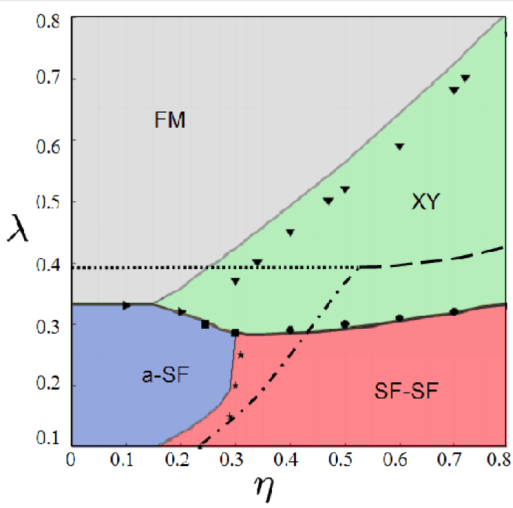
Figure 11: (Color online) Comparative phase diagram for the two-species model as a function $\eta$ and $\lambda$ for $\mu/U=0.25\lambda$ for $t_{1}/U=0.02$. The discrete points represent the phase boundaries as calculated using quantum Monte-Carlo while the colored regions are obtained from the ${\rm O}(t^{2}/U^{2})$ mean field theory. The shape of the markers represent the different phase boundaries; a-SF/SF-SF (stars) ; SF-SF/XY (circles); a-SF/FM (right triangles); FM/XY (up triangles); a-SF/XY (squares). As comparison the phase boundaries obtained using the ${\rm O}(t/U)$ mean field theory are also shown as lines; a-SF/Mott (dotted); a-SF/SF-SF (dash-dotted); SF-SF/Mott (dashed).

First, QMC confirms our suspicion that the appearance of the SS phase for small $\lambda$ is indeed an artifact of the breakdown of the second order perturbation theory at small $\lambda$. Second, comparisons with QMC show that the details of the phase diagram are much better reproduced using the canonical transformation method.

A comparison between the different methods can be seen in Fig. 11 where the phase diagram has been drawn for $\mu/U=0.25\lambda$, $t_{1}/U=0.02$. The dotted, dashed and dash-dotted lines are the phase boundaries as obtained using the ${\rm O}(t/U)$ mean field theory of section III. As can be seen there is a large discrepancy between the location of the phase boundaries as compared to the ${\rm O}(t^{2}/U^{2})$ mean field theory. The discrete set of points represent the phase boundaries obtained by QMC. Comparing the three methods we thus see that the inclusion of ${\rm O}(t^{2}/U^{2})$ effects yields the phase boundaries with great accuracy.

We also find that the Monte Carlo study predicts the a-SF/SF-SF transition to be second order. This validates the result obtained using the canonical transformation method and shows that the expectation of a first order a-SF-SF-SF transition based on ${\rm O}(t/U)$ mean-field theory (Sec. III) was an artifact of omitting ${\rm O}(t^{2}/U^{2})$ corrections.

An interesting prediction, and possible failure, of the ${\rm O}(t^{2}/U^{2})$ mean-field theory is the existence of continuous parameter region having points where four phases meet (cf. the diagrams for $t_{1}=0.04$ and $t_{1}=0.05$ in Fig. 8). However, using QMC for systems of sizes up to $20\times 20$ sites and inverse temperatures $\beta=1500/U$ for parameter values $\mu=0.5\lambda U$, $t_{1}=0.04$, suggests that although the phase boundaries come very close they do not meet at a single point but a small region showing a first order transition between the a-SF and the XY phase seems to remain.

VI Detecting the different phases

The traditional way of examining the existence of superfluidity in trapped boson systems is to switch off the trap, let the cloud of atoms expand freely and image the expanding cloud. The momentum distribution of the atoms inside the trap can then be inferred by looking at their position, or equivalently density, distribution in the expanded cloud. Since the momentum distribution function of the atoms is characterized by the presence/absence of coherence peaks in the superfluid/Mott insulating states, such a measurement serves as a qualitative probe of the state of the atoms inside the trap Bloch1 . In our proposed setup, however, such a simple expansion alone, which can not distinguish between the two species, will not be able to distinguish between all the different phases. Nevertheless, since the two species have different magnetic moments ($m_{F}=-2$ and $m_{F}=-1$), it is possible to separate them during the expansion using a pair of Stern-Gerlach magnets stenger ; blochnew . The expanding cloud will then be separated into two clouds if both species of atoms are present in the system. This, together with the momentum distribution measurement, will qualitatively distinguish between all the phases obtained in this work. To make this statement concrete, let us consider the phase diagram shown in Fig. 9. Here the proposed set of measurements will lead to a) single cloud with no coherence peak (FM phase) or b) single cloud with coherence peak (a-SF phase), or c) two clouds with no coherence peaks (XY phase) or d) two clouds with a coherence peak (SF-SF phase). Thus this methods allows, for instance, the detection of the mixed phases (${\rm MI}_{2}+{\rm SF}_{1}$, a-SF, and SF-SF). It further provides a tool for finding the phase transitions between the Mott phases for $n_{0}=1$. The second order transition from the XY-phase to the FM phase, for example, will be associated with gradual depletion of the atoms in one of the clouds whereas the transition to the AFM phase will be characterized by an abrupt change from a single to a double cloud.

The above mentioned detection technique, however, does not provide any evidence of the isospin order in the Mott states since they can not probe the spatial correlations between the atoms at a lattice scale. Such correlations can be probed, for example, by tilting the optical lattice with a potential gradient Bloch1 . Deep inside the Mott phase, such a potential gradient will excite the system only if ${\mathcal{E}}=E_{dipole}$, where ${\mathcal{E}}$ is the potential energy shift between adjacent lattice due to the field gradient and $E_{dipole}$ is the dipole formation energy Bloch1 ; SKS . The dipole formation energy will sharply change across the phase transition lines between AFM-XY and AFM-FM phases and consequently the peak in the excitation width, measured in Ref. Bloch1, as a function of the applied field gradient, shall show an abrupt shift at the transitions across these phases. In contrast, there will be a gradual shift of the peak position as one moves from the XY to the FM phase. Alternatively, isospin order can also be measured by probing noise correlation of the expanding clouds Han ; Bloch3 ; altman . For example, a transition from the FM to AFM isospin states will be marked by appearance of additional peaks in the noise spectrum at half the reciprocal lattice vector. The detection of the XY phase can also be obtained by the Ramsey spectroscopy technique as suggested in Ref. kuklov1, .

Another possible way of detecting the phases is to image the expanding cloud by passing a linearly polarized laser beam through it. As shown in Ref. carusotto04, , the angle of rotation of the plane of polarization ($\theta_{\rm rot}$) of the outgoing laser beam is proportional to the net $m_{z}$ along the direction of propagation ($x_{\perp}$)of the beam: $\theta_{\rm rot}\sim\int dx_{\perp}m_{z}(x_{\perp})$. $\theta_{rot}$ can then be easily measured by passing the outgoing beam through a crossed polarizer since the intensity of the beam coming out of the crossed polarizer is $I_{-}\sim\sin^{2}\left(\theta_{\rm rot}\right)$. We therefore expect $I_{-}$ to jump discontinuously across any first order transitions such as FM-AFM or XY-ASF phase boundaries and gradually change across second order transitions such as the FM-a-SF or XY-2SF phase boundaries. Of course, such measurements have to be supplemented with momentum distribution function measurement to distinguish between the superfluid and Mott phases.

A brief comment on system preparation and validity of use of grand canonical ensemble is in order here. One should note that although use of a grand canonical ensemble in the single species case is a good approximation due to the presence of a confining potential (in this case the confining potential produces spatial inhomogeneities in the filling factor and some of the outer regions will act like a particle reservoir for the inner region), this is not necessarily the case in the two species system and other means may have to be sought.

VII Conclusions

In conclusion, we have studied the MI-SF transition in a consisting of two species of ultracold atoms in an optical lattice in a previously unexplored parameter region. We have used an ${\rm O}(t/U)$ mean-field theory to explain the qualitative features of the transition in most regions of the phase diagram. This is followed by incorporating the ${\rm O}(t^{2}/U^{2})$ exchange effects using a canonical transformation method and a quantum Monte Carlo calculation. All of these methods show that the superfluid-insulator transition can occur with either depopulation of species $2$ (a-SF phase) or simultaneous onset of superfluidity of both species (SF-SF phase) or Mott insulator of species $2$ coexisting with superfluid of species $1$ (${\rm MI}_{2}+{\rm SF}_{1}$ phase) and can be first order in large regions of the phase diagram. We have also shown that, whereas some qualitative features of the SI transition can be obtained from ${\rm O}(t/U)$ mean-field theory, incorporating the ${\rm O}(t^{2}/U^{2})$ corrections is necessary to deduce the details of the phase diagram and order of the transitions between the phases. Our quantum Monte Carlo study lends strong support to the above-mentioned results and also shows screening of bosons of species $2$ in the SF-SF phase. We also discussed possible experimental tests of some of our predictions.

Appendix A

Here we briefly sketch the derivation of $H^{\ast}$ (Eq. LABEL:hamf) starting from Eq. 21. To do this we show the detailed derivation of two terms $H_{1}=[iS,H_{0}]$ and $H_{2}=[iS,T_{\sigma}]$. The derivations of all other terms follow in a similar fashion.

VII.1 $H_{1}$

To compute $H_{1}$, we use Eq. 20 to expand $S$ and write

$$[iS,H_{0}] = -\frac{1}{\lambda U}\sum_{\sigma}\left[[\lambda P_{\sigma}^{S}+P_{\sigma}^{D},T_{\sigma}],H_{0}\right]$$ (23)

$$= -\frac{1}{\lambda U}\sum_{\sigma}\Big{[}\left(\lambda P_{\sigma}^{S}T_{\sigma}+P_{\sigma}^{D}T_{\sigma}\right.$$

$$\left.-\lambda T_{\sigma}P_{\sigma}^{S}-T_{\sigma}P_{\sigma}^{D}\right),\,H_{0}\Big{]}$$

Now consider the first term in the commutator in Eq. 23. Noting that the projection operator $P_{\sigma}$ always projects onto the states $|1,0>$ or $|0,1>$, we see that we can write

$$P_{\sigma}^{S}T_{\sigma}H_{0}-H_{0}P_{\sigma}^{S}T_{\sigma} = UP_{\sigma}^{S}T_{\sigma}$$ (24)

This is an operator identity guaranteed by the construction of the projection operator $P_{\sigma}$. Other terms in Eq. 23 can be written in a similar fashion and we have

$$H_{1} = -\sum_{\sigma}\left(P_{\sigma}^{S}T_{\sigma}+P_{\sigma}^{D}T_{\sigma}+T_{\sigma}P_{\sigma}^{S}+T_{\sigma}P_{\sigma}^{D}\right)$$ (25)

$$= -\sum_{\sigma}\left(P_{\sigma}T_{\sigma}+T_{\sigma}P_{\sigma}^{S}\right)=-\sum_{\sigma}T_{\sigma}^{1}$$

where in obtaining the last line we have again used the properties of the projection operators $P_{\sigma}^{S}$. Combining Eqs. 18, 25 and 20, we get the second term in Eq. LABEL:hamf.

VII.2 $H_{2}$

Now we consider the term $H_{2}=[iS,\sum_{\sigma}T_{\sigma}^{1}]$. For this, as we shall see, it is useful to define the operator ${\mathcal{M}}_{\sigma}=P_{\sigma}T_{\sigma}+T_{\sigma}P_{\sigma}$. Then one can write, using Eq. 20

$$H_{2} = -\frac{1}{\lambda U}\sum_{\sigma,\sigma^{\prime}}\left[[P_{\sigma}^{\lambda}T_{\sigma}],{\mathcal{M}}_{\sigma^{\prime}}\right]$$ (26)

Note that unlike $H_{1}$, here the sum extends over two different bonds $\sigma$ and $\sigma^{\prime}$. Consequently, expansion of Eq. 26 leads to terms which can be classified into two categories.The first type of terms involves two hopping operators $T_{\sigma}$ on the same bond while the second involves the hopping operators on the different bonds:

$$H_{2} = H_{2a}+H_{2b}$$

$$H_{2a} = -\frac{1}{\lambda U}\sum_{\sigma}\left[[P_{\sigma}^{\lambda},T_{\sigma}],{\mathcal{M}}_{\sigma}\right]$$ (27)

$$H_{2b} = \frac{1}{\lambda U}\sum_{\sigma}\sum_{j}\left[[P_{\sigma}^{\lambda},T_{\sigma}],{\mathcal{M}}_{\sigma+j}\right]$$ (28)

where the sum over $j$ extend over the bonds which are nearest neighbors to $\sigma$.

We first consider $H_{2a}$. We expand the operators ${\mathcal{M}}_{\sigma}$ and $P_{\sigma}^{\lambda}$ and use the relation $[P_{\sigma},P_{\sigma}^{\lambda}]=0$. Also, we note that all terms of the form $P_{\sigma}^{1}T_{\sigma}P_{\sigma}^{0}T_{\sigma}$ in such an expansion vanish identically. After some straightforward algebra, one obtains

$$H_{2a} = -\frac{1}{\lambda U}\left[P_{\sigma}^{\lambda}T_{\sigma}^{2}P_{\sigma}+P_{\sigma}T_{\sigma}^{2}P_{\sigma}^{\lambda}-2T_{\sigma}P_{\sigma}^{\lambda}T_{\sigma}\right]$$ (29)

Note that the first two terms of Eq. 29 represent second order virtual hopping processes and thus give the $t^{2}/U$ terms responsible for the isospin ordering of the Mott phases, while the third term represents two particle-hopping across a bond with an intermediate virtual state of one particle on each side of the bond.

Next we come to computation of $H_{2b}$. We again expand out the operators as before. Here, the crucial identity is that any terms of the form $P_{\sigma}T_{\sigma}P_{\sigma+j}^{\lambda}T_{\sigma+j}$ or $P_{\sigma+j}T_{\sigma+j}P_{\sigma}^{\lambda}T_{\sigma}$ vanish as long as $\sigma$ and $\sigma+j$ denotes nearest-neighbor bonds. Using this, one gets

$$H_{2b} = -\frac{1}{\lambda U}\sum_{\sigma}\sum_{j}\Big{(}P_{\sigma}^{\lambda}T_{\sigma}T_{\sigma+j}P_{\sigma+j}$$ (30)

$$-T_{\sigma}P_{\sigma}^{\lambda}P_{\sigma+j}T_{\sigma+j}+{\rm h.c.}\Big{)}$$

The other term $\left[iS,\left[iS,H_{0}\right]\right]$ in Eq. 21 can be computed in a similar fashion. Using all these results, we finally obtain Eq. LABEL:hamf.

References

- (1)
- (2) M. Greiner, O. Mandel, T. Esslinger, T.W. Hansch, and I. Bloch, Nature (London) 415, 39 (2002).
- (3) C. Orzel, A.K. Tuchman, M.L. Fenselau, M. Yasuda, and M.A. Kasevich, Science 291, 2386 (2001).
- (4) For a review, see Chapter 11 in Quantum Phase Transitions, S. Sachdev,(Cambridge University Press, Cambridge, England, 1999).
- (5) O. Mandel , Nature (London) 425, 937 (2003).
- (6) For a review on internal states of atoms in Bose Einstein condensates, see A. Legget, Rev. Mod. Phys. 73, 307 (2001).
- (7) D. Jaksch , Phys. Rev. Lett. 82, 1975 (1999)
- (8) G. K. Brennen et al., Phys. Rev. Lett. 82, 1060 (1999).
- (9) E. Altman et al., New Journal of Physics 5, 113 (2003).
- (10) L-M. Duan, E. Demler, and M. Lukin, Phys. Rev. Lett. 91, 090402 (2003).
- (11) A. Kuklov and B. Svistunov, Phys. Rev. Lett. 90, 100401 (2003); A. Kuklov, N. Prokof’ev, and B. Svistunov, Phys. Rev. Lett. 92, 050402 (2004).
- (12) G.-H. Chen and Y.-S. Wu, Phys. Rev. A 67, 013606 (2003).
- (13) S.M. Girvin, Proc. 11th Int. Conf. on Recent Progress in Many-Body Theories, ed. R. F. Bishop, T. Brandes, K.A. Gernoth, N.R. Walet, and Y. Xian, Advances in Quantum Many Body Theory (World Scientific, 2002) [cond-mat/0108181].
- (14) K. Moon, H. Mori, Kun Yang, S.M. Girvin, A.H. MacDonald, L. Zheng, D. Yoshioka, and Shou-Cheng Zhang, “Spontaneous Inter-layer Coherence in Double-Layer Quantum-Hall Systems: Charged Vortices and Kosterlitz-Thouless Phase Transitions”, Phys. Rev. B5151381995.
- (15) G.G. Bartouni and R.S. Scalettar, Phys. Rev. Lett. 84 1599 (2000).
- (16) This way of formulating the mean-field theory can be shown to be equivalent to the Hubbard-Stratonovitch decoupling approach, provided the isospin flip process is taken into account in computation of the on-site Green function.
- (17) W. Krauth and N. Trivedi, Phys. Rev. B 14, 627 (1991); W. Krauth, N. Trivedi and D. Ceperley, Phys. Rev. Lett. 67, 2307 (1991).
- (18) A. H. MacDonald, S. M. Girvin, and D. Yoshioka, Phys. Rev. B 41, 2565 (1990); ibid. 37, 9753 (1988).
- (19) A. L. Chernyshev , cond-mat/0407255.
- (20) A.W. Sandvik and J. Kurkijärvi, Phys. Rev. B 43, 5950 (1991).
- (21) A.W. Sandvik, Phys. Rev. B 59, R14 157 (1999).
- (22) O. F. Syljuåsen, Phys. Rev. A 67, 046701 (2003).
- (23) E.L. Pollock and D.M. Ceperley, Phys. Rev. B 36, 8343 (1987).
- (24) N. Prokofiev and B. Svistunov, cond-mat/0301205.
- (25) J. Stenger et al. Nature 396, 345 (1998).
- (26) A. Widera et al., cond-mat/0505492 (unpublished).
- (27) S. Sachdev, K. Sengupta, and S.M. Girvin, Phys. Rev. B 66, 075128 (2002).
- (28) R. Hanbury Brown and R. Twiss, Nature 177, 27 (1956).
- (29) S. Folling Nature 434, 481 (2005).
- (30) E. Altman, E. Demler, and M. D. Lukin, Phys. Rev. A 70, 013603 (2004).
- (31) I. Carusotto and E. J. Muller, J. Phys. B. 37, s115-s125 (2004).