Scale Free Cluster Distributions from Conserving Merging-Fragmentation Processes.

Abstract

We propose a dynamical scheme for the combined processes of fragmentation and merging as a model system for cluster dynamics in nature and society displaying scale invariant properties. The clusters merge and fragment with rates proportional to their sizes, conserving the total mass. The total number of clusters grows continuously but the full time-dependent distribution can be rescaled over at least 15 decades onto a universal curve which we derive analytically. This curve includes a scale free solution with a scaling exponent of $-3/2$ for the cluster sizes.

The combination of the two basic dynamical processes, fragmentation and merging, is of importance in a number of situations of nature and society. Examples range from the dynamical evolution of companies where mergers and split-offs are important ingredients in daily business life. Empirical observations of US companies indicates that their sizes follow a scale invariant distribution company . Another example comes from the dynamics of grain boundaries in crystal growth where neighboring grains might merge at the same time as other grains fragment away from larger crystals. In crystal growth diffusion of grain boundaries can also be of importance in an interplay with merging and fragmentation is ; ferkinghoff ; poul . Fish schools are known to merge together resulting in scale free distribution up to a school size after which it becomes exponentially distributed bonabeau . In polymer physics merging and fragmentation are of importance in relation to gel and shattering transitions ziff ; other examples are aerosols frielander and scaler transport melzak fragmentation/coagulation (i.e. merging) models (see e.g. drake ; leyvraz for reviews on merging/fragmentation processes). Finally, we mention an astrophysical application for the formation of stars and interstellar clouds source .

It is known empirically that the resulting cluster distribution in some of the above mentioned examples has scale free behavior. There has however, to the best of our knowledge, neither been proposed an analytical theory nor any fundamental model studies of these scale free distributions in closed systems driven by combined merging/fragmentation processes. In this Letter we respond to this challenge by introducing a dynamical model system where clusters merge and fragment with rates proportional to the sizes, conserving the total mass of the system. Indeed, some previous models have been introduced to explain the scale free behavior but they relay on a source term for small cluster sizes and thus represent systems with non-conserved mass source ; vicsek ; family ; ernst ; zheng ; minn . The dynamics of our model self-organizes the system to possess a stationary “continuous” scale free cluster size distribution over many decades and up to a characteristic size above which only the largest clusters will be situated. We introduce an analytical theory for the model based on Smoluchowski’s continuous cluster fragmentation and coagulation (i.e. merging) model smoluchowski1916 . We show that this model with “mass” kernels exhibits an exact scale invariant solution of the cluster distribution, $n(x)\sim x^{-3/2}$, at a critical point where merging processes balance the fragmentation processes. In this solution, it turns out that there is a gap in the distribution above which only a few large clusters exist. The scaling exponent $-\frac{3}{2}$ is in agreement with distributions of fish schools bonabeau and many critical branching processes branching , for instance.

Our model is defined in terms of ${\cal N}$ clusters $\{\tilde{x}_{i}\}_{i=1}^{{\cal N}}$ each of size $\tilde{x}_{i}$, where tilde ($\tilde{~{}}$) in the following is used for dimensionfull quantities. The total initial mass of all clusters is thus $\tilde{M}=\sum_{i=1}^{\cal N}\tilde{x}_{i}$. At time $\tilde{t}$ the clusters $i$ and $j\neq i$ are chosen to merge with a rate $K_{ij}=\beta\tilde{x}_{i}\tilde{x}_{j}$ and the cluster $k$ is chosen to fragment with the rate $F_{k}=f\tilde{x}_{k}$. The size of the two clusters resulting from a fragmentation is chosen randomly (ie. with a uniform distribution). The average time $\delta\tilde{t}$ for the next merging or fragmentation event to occur is obtained from the total merging and fragmentation rates, $\tilde{k}_{\mbox{merge}}$ and $\tilde{k}_{\mbox{frag}}$, as $\delta\tilde{t}=(\tilde{k}_{\mbox{frag}}+\tilde{k}_{\mbox{merge}})^{-1}$, where

$$\tilde{k}_{\mbox{merge}}=\sum_{i}\sum_{j>i}K_{ij}=\beta/2\left(\tilde{M}^{2}-\tilde{M}_{2}\right).$$

and

$$\tilde{k}_{\mbox{frag}}=\sum_{i}F_{i}=f\tilde{M}$$

and $\tilde{M}_{2}=\sum_{i}\tilde{x}_{i}^{2}$ is the second moment of the distribution. In time-step $\delta\tilde{t}$ the merging and fragmentation processes are thus associated with the probabilities $p_{ij}=K_{ij}\delta\tilde{t}$ and $p_{k}=F_{k}\delta\tilde{t}$, respectively. Since the processes preserve the total mass we can express the dynamics in terms of the dimensionless quantities,

$$\begin{array}[]{rlrl}x&=\frac{\tilde{x}}{\tilde{M}},&t&=\tilde{t}(f\tilde{M})^{-1}\\ k_{\mbox{frag}}&=1,&k_{\mbox{merge}}&=b/2(1-M_{2}),\\ \end{array}$$ (1)

where $b=\tilde{M}\beta/f$ and $M_{2}=\sum_{i}x_{i}^{2}$.

In Fig. 1 we show the cumulative distribution, $N(x,t)=\sum_{i}\Theta(x_{i}(t)-x)$, for a simulation with $b=3$ at various times $t$. Here, $\Theta(x)$ is the Heaviside function, $\Theta(x)=1$ for $x\geq 0$ and $\Theta(x)=0$ for $x<0$. At each time $t$, the fragments larger than a characteristic cross-over scale, $x\gg x_{c}(t)$, are distributed according to a power law, $N(x)\sim x^{\alpha}$ with $\alpha=-1/2$. As seen in the figure, $x_{c}(t)\rightarrow 0$ for $t\rightarrow\infty$, implying the existence of a scale invariant state which extends to smaller and smaller scales as time increases. The same data are shown in Fig. 2 with $N(x,t)$ as function of $t$ for various values of $x$. Interestingly, the total number of domains ${\cal N}(t)=N(0,t)$ grows as ${\cal N}(t)\sim t^{\gamma}$ with the power $\gamma=-\alpha=1/2$. For each $x>0$, the distribution is time-dependent, $N(x,t)\sim t^{1/2}$, for times smaller than a characteristic cross-over time $t\ll t_{c}(x)$, and becomes time independent, $N(x,t)=N(x)$ for $t\gg t_{c}(x)$.

Simulations for other values of $b>2$ lead to distributions, $N(x)$, and evolutions ${\cal N}(t)$ which are very close to power-laws, $N(x)\sim x^{\alpha(b)}$ and ${\cal N}(t)\sim t^{\gamma(b)}$ with $b$-dependent exponents $\gamma(b)$ and $\alpha(b)$ satisfying $\gamma(b)=-\alpha(b)$ usnew . Nonetheless, only at $b=3$ does the scale-invariant behavior become exact. For $b\leq 2$, the maximum mass $m_{1}$ approaches $m_{1}=0$ as $t\rightarrow\infty$ usnew , implying that no time-independent solution exists in this parameter region.

Figure 1: Cumulative distribution, $N(x,t)$, of the fragment sizes $x$ at various times, $t=5\cdot 10^{7},2\cdot 10^{8},10^{9},5\cdot 10^{9},2.5\cdot 10^{10}$. The thick solid line is the average cumulative distribution, $N(x)$, for $x>10^{-9}$ taken over times $t>10^{9}$. At any instant, $N(x,t)$ displays a characteristic cross-over from an almost flat distribution to a scale-invariant distribution, $N(x)\sim x^{-1/2}$, at larger $x$. As time goes the scale free part of the distribution extends to smaller and smaller scales. The inset shows the behavior of $N(x)$ in the large part of the mass spectrum. The dotted line is the simple scaling form, $N_{1}(x)=Ax^{-1/2}$, with $A\approx 0.9$, and the dashed line is the predicted cumulative distribution, $N_{0}(x)=A\left(x^{-1/2}-3/16A\pi\right)$ (see text). The dots in the figure represent the typical size ($50\%$ fractile) of the 10 largest fragments, ie. points corresponding to $N(m_{i})=i-1/2$, where $m_{i}$ the the typical size of the $i$’th largest fragment. The predicted cumulative distribution, $N_{0}$, deviates from data around $x=l\sim 0.1$ corresponding to the typical size of the third largest fragment, $m_{3}\approx 0.09$. The naive scaling form, $N_{1}$, deviates from data already around $x\sim 0.02$.

Figure 2: Cumulative distribution, $N(x,t)$, as function of time $t$ at various sizes, $x=0,10^{-10},10^{-9},10^{-8},10^{-7},10^{-6}$. For each positive value of $x$, $N(x,t)$ displays a cross-over from a power law $N(x,t)\sim t^{1/2}$ at short times to a constant, $N(x,t)=N(x)$, at large times.

To analyze the origin of the scale invariant solution we express the dynamics in terms of Smoluchowski’s continuous cluster fragmentation and coagulation (i.e. merging) model smoluchowski1916 . We have previously presented this type of rate equations including diffusion, fragmentation and coagulation (ie. merging) terms, which are of relevance for dynamical processes of ice crystals, alpha helices and macromolecules is ; ferkinghoff ; poul . Let $n(x,t)=-\partial_{x}N(x,t)$ denote the number density of clusters of size $x$ at time $t$. Smoluchowski’s fragmentation-coagulation model describes the dynamics of clusters subject to fragmentation and coagulation processes. If $K(x,x^{\prime})$ and $F(x,x^{\prime})$ represent, respectively, the rate of coagulating two clusters of size $x$ and $x^{\prime}$ into a cluster of size $x+x^{\prime}$ and the rate of fragmenting a cluster of size $x+x^{\prime}$ into two clusters of size $x$ and $x^{\prime}$, the model takes the form

$$\partial_{t}n(x,t) = -n(x,t)\int_{0}^{x}F(x-x^{\prime},x^{\prime})dx^{\prime}$$ (2)

$$+ 2\int_{x}^{L}F(x,x^{\prime})n(x+x^{\prime},t)dx^{\prime}$$

$$+ \frac{1}{2}\int_{0}^{x}K(x-x^{\prime},x^{\prime})n(x-x^{\prime},t)n(x^{\prime},t)dx^{\prime}$$

$$- n(x,t)\int_{0}^{L}K(x,x^{\prime})n(x^{\prime},t)dx^{\prime},$$

where $L$ represents the largest possible cluster size. Using dimensionless quantities, Eq. (1), our model corresponds to the choice, $L=1$, $F(x,x^{\prime})=1$ and $K(x,x^{\prime})=b\cdot(x\cdot x^{\prime})$. The general form of the merging-fragmentation process then reads

$$\partial_{t}n(x,t) = -xn(x,t)+2N(x,t)$$ (3)

$$+ \frac{b}{2}\int_{0}^{x}x^{\prime}(x-x^{\prime})n(x^{\prime},t)n(x-x^{\prime},t)dx^{\prime}$$

$$- bxn(x,t),$$

where $N(x,t)=\int_{x}^{1}n(x^{\prime},t)dx^{\prime}$ and the mass normalization, $\int_{0}^{1}xn(x,t)dx=1$, has been used. We note that the representation of the dynamics in terms of a density function, $n(x,t)$, is only accurate if the typical spacing $\delta x$ between clusters of size $\sim x$, satisfies $\delta x\ll x$, implying $x\ll 1$. In particular, the assumption of smoothness is important for the integral expressions for the fragment gain and loss due to merging to be correct. These terms erroneously include ’self-merging’ processes, $x+x\rightarrow 2x$, as well, thereby giving an addition to the actual merging rates which can only be ignored in the limit $\delta x\ll x$. Eq. (2-3) are therefore not adequate for the dynamics of fragments carrying a large fraction of the total mass, as the error in the merging rates become non-negligible here and fail to guarantee total mass conservation. In fact, Eq. (2), is only mass conserving in the limit $L\rightarrow\infty$, for which the particular rescaling to dimensionless quantities in Eq. (1), can not be done. In the following, we will tentatively assume the continuous representation to be correct up to some length scale $l\ll 1$ and seek analytical solutions to Eq. (3) in this regime.

Critical points are generally associated with scale invariant behavior. For cluster dynamics with merging and fragmentation, scale invariance has been obtained previously in vicsek ; family ; ernst ; source ; zheng , although all under somewhat different circumstances i.e. with source terms and thus not in a closed system. Therefore, we are searching for stationary scale-invariant solutions on the form, $n_{0}(x)\sim x^{\alpha-1}$ or $N_{0}(x)=Ax^{\alpha}+C$. Inserting this scaling relation into Eq. (3) we obtain

$$0 = -Ax^{\alpha}\left(\alpha+2+b\alpha\right)+2C$$ (4)

$$+ \frac{b}{2}(\alpha A)^{2}x^{(2\alpha+1)}*B(\alpha+1,\alpha+1)$$

where $B(\alpha+1,\alpha+1)$ is the Beta function $B(\alpha+1,\alpha+1)=\Gamma(\alpha+1)\Gamma(\alpha+1)/\Gamma(2\alpha+2)$ under the assumption that $\alpha+1>0$. Power counting arguments now easily gives that only two values for the exponent is possible, namely $\alpha=-1$ or $\alpha=-1/2$. The value $\alpha=-1$, however will ruin the assumption $\alpha+1>0$ and is inconsistent with the finite mass of the system comment . Thus we come to the conclusion that there is only one scale invariant solution to Eq. (3), namely $n_{0}(x)=A/2x^{-3/2}$, which becomes an exact solution provided that $\alpha+2+b\alpha=0$ or $b=3$. Also, stationarity requires $C=-3/16A^{2}\pi$ so the total number of clusters larger than $x$ for $x_{c}(t)\ll x<l$, is simply

$$N_{0}(x)=A\left(x^{-1/2}-3/16A\pi\right).$$ (5)

The actual value of $A$ depends on how much of the total mass is situated in the discrete part of the spectrum given by the few fragments with $x>l$, $\int_{0}^{l}xn_{0}(x)dx+\sum_{x_{i}>l}x_{i}=1$. Setting (incorrectly) $l=1$ implies $A=1$. To assess the scaling behavior in the large mass limit, we show in the inset of Fig. 1 the average cumulative distribution for $x>10^{-3}$ where size fluctuations becomes noticeable. Using a fitted value of $A\approx 0.9$, the analytical solution, Eq. (5) is observed to be accurate all the way up to $l\sim 0.1$, as expected from the condition $l\ll 1$. The value for $l$ corresponds to the typical size ($50\%$ fractile) of the third largest fragment, $m_{3}\approx 0.09$, effectively meaning that only the two largest fragments belong to the discrete spectrum. In fact, the distribution $N(x)$ has significant gaps around the two largest fragments, e.g. $\delta x=1/2(m_{1}-m_{3})\approx 1/2(0.47-0.09)=0.19$, compared to the small differences $\delta x\ll 1$ around all other fragments.

Eq. (3) suggests that the full time dependent distribution, $N(x,t)$ can be expressed in the form $N(x,t)=t^{\gamma}\phi(xt)+C$. Indeed, setting $z=xt$ one obtains from Eq. (3)

$$-t^{\gamma}\left((\gamma+1)\phi^{\prime}(z)+z\phi^{\prime\prime}(z)\right)=$$ (6)

$$t^{\gamma}\left(z\phi^{\prime}(z)+2\phi(z)+bz\phi^{\prime}(z)\right)+$$

$$C+1/2t^{2\gamma-1}b\int_{0}^{z}z^{\prime}(z-z^{\prime})\phi^{\prime}(z)\phi^{\prime}(z-z^{\prime})dz^{\prime},$$

which is a function of $z$ only, provided that either $\gamma=1$ or $\gamma=1/2$ and $1/2b\int_{0}^{z}z^{\prime}(z-z^{\prime})\phi^{\prime}(z)\phi^{\prime}(z-z^{\prime})dz^{\prime}\approx-C$. Requiring $N(x,t)=N_{0}(x)$ for $x\gg x_{c}(t)$, implies $\phi(z)\sim z^{\alpha}$ for large $z$ and $\gamma=-\alpha=1/2$. Neglecting the two last terms on the rhs. of Eq. (6), one can obtain the distribution for all $z$ by solving the linear differential equation,

$$-3/2\phi^{\prime}(z)-z\phi^{\prime\prime}(z)=z\phi^{\prime}(z)+2\phi(z)+3z\phi^{\prime}(z),$$

where $\gamma=1/2$ and $b=3$ has been inserted. The solution yields $\phi(z)=a_{1}z^{-1/2}+a_{2}\psi(z)$, where $\psi(z)=\frac{\mbox{erf}(2\sqrt{z})}{\sqrt{z}}$ and $\mbox{erf}(y)$ is the error function, $\mbox{erf}(y)=\frac{2}{\sqrt{\pi}}\int_{0}^{y}e^{-r^{2}}dr$. The integration constants, $a_{1}$ and $a_{2}$, can be found from the known behavior of $\phi(z)$ in the limits $z\rightarrow\infty$ and $z\rightarrow 0$. Requiring $\phi(z)\rightarrow\mbox{const}$ for $z\rightarrow 0$ implies $a_{1}=0$ and since $\psi(z)\rightarrow z^{-1/2}$ for large $z$, one obtains $a_{2}=A$. For this solution the convolution term in Eq. (6) is bounded, $0\leq\int_{0}^{z}z^{\prime}(z-z^{\prime})\phi^{\prime}(z)\phi^{\prime}(z-z^{\prime})dz\leq B(1/2,1/2)$ and has a weak $z$-dependence which is negligible at larger times. The final form of $N(x,t)$ then reads

$$N(x,t)=t^{1/2}\phi(xt)-3/16A^{2}\pi,~{}~{}~{}~{}\phi(z)=A\frac{\mbox{erf}(2\sqrt{z})}{\sqrt{z}}.$$ (7)

In Figure 3, we show $(N(x,t)+3/16A^{2}\pi)t^{-1/2}$, as function of $z=xt$ for 50 distributions taken in the time interval $10^{7}\leq t\leq 2.5\cdot 10^{10}$. The thick solid line is the predicted functional form, $\phi(z)$ which agrees perfectly with data. The full time dependent solution, Eq. (7), of the combined process of fragmentation and coagulation is the main result of this Letter. The spread around $\phi(xt)$ for large values of $xt$ is caused by noticeable fluctuations of the largest fragments of the distribution. Eq. (7) also shows that the characteristic cross-over scale, $x_{c}(t)$ (above which the the system is stationary and scale free), goes with time as $x_{c}(t)\sim t^{-1}$. Conversely, had we introduced a smallest length scale, $\delta$, in the system, we would expect convergence to a full stationary distribution after time $t\sim\delta^{-1}$, displaying scale invariance in the region $\delta\ll x\ll 1$.

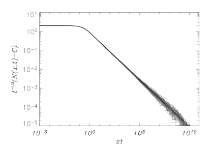
Figure 3: The rescaled cumulative distribution, $t^{-1/2}(N(x,t)-C)$, where $C=-3/16A^{2}\pi$, Eq. (7), as function of $z=xt$ taken at 50 different times in the interval $10^{7}\leq t\leq 2.5\cdot 10^{10}$. In black solid line is shown the predicted functional form $\phi(z)=A\frac{\mbox{erf}(2\sqrt{z})}{\sqrt{z}}$.

Let us now comment on conserved versus non-conserved merging/fragmentation processes. Imagine a simulation where clusters, when becoming too large, above the scale $\tilde{l}$, are disregarded and the total mass is not conserved. From these kind of simulations we have observed a transient scale invariant cluster size distribution, $n(x)\sim x^{-2}$, consistent with simple power counting of Eq. (3) (corresponding to $\alpha=-1$). However, the total mass will eventually become smaller than $\tilde{l}$, after which the dynamics again is mass conserving leading to the $n(x)\sim x^{-3/2}$ distribution. The $-2$ versus $-3/2$ solutions might be relevant in discussions of data from a variety of systems depending on the degree to which they are mass conserving. In the case of American companies, the exponent of the scale invariant distribution is closer to $-2$ than $-3/2$ company , which in the light of our model indicates that the total wealth of companies is not conserved.

In this letter we have presented a general formalism for scale invariant and critical behavior in systems where merging balances fragmentation. We have proposed a dynamical model where the merging/fragmentation processes drive the system into a critical state. From an analytical solution of Smoluchowski’s equation we show that this scale invariant state represents a unique part of the cluster distribution. We suggest that the proposed principle could be the dynamical background behind many scale free systems of society and nature.

We are grateful to S. Manrubia, S. Maslov and K. Sneppen for useful discussions.

References

- (1) D. Zajdenweber, Fractals 3, 601 (1995).
- (2) J. Mathiesen, J. Ferkinghoff-Borg, M. H. Jensen, M. Levinsen, P. Olesen, D. Dahl-Jensen and A. Svensson, J. Glaciology 50, 325 (2004).
- (3) J. Ferkinghoff-Borg, M. H. Jensen, J. Mathiesen, P. Olesen and K. Sneppen, Phys. Rev. Lett. 91. 266103-266106 (2003).
- (4) P. Olesen, J. Ferkinghoff-Borg, M. H. Jensen, J. Mathiesen, Phys. Rev. E, in press.
- (5) E. Bonabeau and L. Dagorn, Phys. Rev. E 51, R5220 (1995); E. Bonabeau, L. Dagorn, and P. Fréon, J. Phys. A 31, L731 (1998); E. Bonabeau, L. Dagorn, and P. Fréon, Proc. Natl. Acad. Sci. (USA), 96, 4472 (1999).
- (6) R. M. Ziff, Kinetics of polymerization, J. Stat. Phys. 23, 241-263 (1980).
- (7) S. K. Frielander, Smoke, dust and haze: fundamentals of aerosol dynamics, Wiley, New York (1977).
- (8) Z. A. Melzak, Trans. Amer. Math. Soc. 85, 547-560 (1957).
- (9) R. L. Drake. A general mathematical survey of the coagulation equation. In G.M. Hidy and J.R. Brock, editors, Topics in Current Aerosol Research (Part 2), pages 201-376. Pergamon Press, Oxford (1972).
- (10) F. Leyvraz, “Scaling theory and exactly solved models in the kinetics of irreversible aggregation”, Phys. Rep. 383, 95 (2003).
- (11) G.B. Field and W.C. Saslaw, Astrophys. J. 142, 568 (1965).
- (12) P. Minnhagen, M. Rosvall, K. Sneppen and A. Trusina, Physica A 340, 725 (2004).
- (13) T. Vicsek and F. Family, Phys.Rev. Lett. 52, 1669 (1984).
- (14) F. Family, P. Meakin and J.M. Deutch, Phys.Rev. Lett. 57, 727 (1986).
- (15) P.G.J. van Dongen and M.H. Ernst, Phys. Rev. Lett. 54, 1396 (1985). H. Hayakawa, J. Phys. A 20, L801 (1987).
- (16) D. Zheng, G.J. Rodgers and P.M. Hui, Physica A 310, 480 (2002).
- (17) M. von Smoluchowski, Phys. Z. 17, 557, 585 (1916).
- (18) T.E. Harris, “The theory of branching processes”, Springer-Verlag, Berlin (1963).
- (19) J. Ferkinghoff-Borg, M. H. Jensen, J. Mathiesen, P. Olesen, unpublished (2005).
- (20) To be precise, implies that the total mass in the scale-invariant region, , becomes as the lower scale, , tends to zero at large times.