Disordered ultracold atomic gases in optical lattices: A case study of Fermi-Bose mixtures

Abstract

We present a review of properties of ultracold atomic Fermi-Bose mixtures in inhomogeneous and random optical lattices. In the strong interacting limit and at very low temperatures, fermions form, together with bosons or bosonic holes, composite fermions. Composite fermions behave as a spinless interacting Fermi gas, and in the presence of local disorder they interact via random couplings and feel effective random local potential. This opens a wide variety of possibilities of realizing various kinds of ultracold quantum disordered systems. In this paper we review these possibilities, discuss the accessible quantum disordered phases, and methods for their detection. The discussed quantum phases include Fermi glasses, quantum spin glasses, ”dirty” superfluids, disordered metallic phases, and phases involving quantum percolation.

I Introduction

I.1 Disordered systems

Since the discovery of the quantum localization phenomenon by P.W. Anderson in 1958 pwa , disordered and frustrated systems have played a central role in condensed matter physics. They have been involved in some of the most challenging open questions concerning many body systems (cf. cusack ; balian ; chow ). Quenched (i.e., frozen on the typical time scale of the considered systems) disorder determines the physics of various phenomena, from transport and conductivity, through localization effects and metal-insulator transition (cf. anderson ), to spin glasses (cf. parisi ; stein ; sachdev ), neural networks (cf. amit ), percolation percbook ; spiperc , high $T_{c}$ superconductivity (cf. Auerbach ), or quantum chaos haake . One of the reasons why disordered systems are very hard to describe and simulate is related to the fact that, usually, in order to characterize the system, one should calculate the relevant physical quantities averaged over a particular realization of the disorder. Analytical approaches require the averaging of, for instance, the free energy, which (being proportional to the logarithm of the partition function in the canonical ensemble) is a very highly nonlinear function of the disorder. Averaging requires then the use of special methods, such as the replica trick (cf. parisi ), or supersymmetry method efetov . In numerical approaches this demands either simulating very large samples to achieve “self-averaging”, or numerous repetitions of simulations of small samples. Obviously, this difficulty is particularly important for quantum disordered systems. Systems which are not disordered but frustrated (i.e., unable to fulfill simultaneously all the constrains imposed by the Hamiltonian), lead very often to similar difficulties, because quite often they are characterized at low temperature by an enormously large number of low energy excitations (cf. lhuillier ). It is thus desirable to ask whether atomic, molecular physics and quantum optics may help to understand such systems. In fact, very recently, it has been proposed how to overcome the difficulty of quenched averaging by encoding quantum mechanically in a superposition state of an auxiliary system, all possible realizations of the set of random parameters belen . In this paper we propose a more direct approach to the study of disorder: direct realization of various disordered models using cold atoms in optical lattices.

I.2 Disordered ultracold atomic gases

In the recent years there has been an enormous progress in the studies of ultracold weakly interacting lev , as well as strongly correlated atomic gases. In fact, present experimental techniques allow to design, realize and control in the laboratory various types of ultracold interacting Bose or Fermi gases, as well as their mixtures. Such ultracold gases can be transfered to optical lattices and form a, practically perfect, realization of various Hubbard models hubbards . This observation, suggested in the seminal theory paper by Jaksch et al. jaksch in 1998, and confirmed then by the seminal experiments of M. Greiner et al. bloch , has triggered an enormous interest in the studies of strongly correlated quantum systems in the context of atomic and molecular lattice gases.

It became soon clear that one can introduce local disorder and/or frustration to such systems in a controlled way using various experimentally feasible methods. Local quasi-disorder potentials may be created by superimposing superlattices incommensurable with the main one to the system. Although strictly speaking such a superlattice is not disordered, its effects are very similar to those induced by the genuine random potentials boseglass ; keith ; laurent . Controlled local truly random potentials can be created by placing a speckle pattern on the main lattice grynberg ; dainty . As shown in Ref. boseglass , for a system of strongly correlated bosons located in such a disordered lattice, both methods should permit to achieve an Anderson-Bose glass fisher , provided that the correlation length of the disorder $L_{dis}$ is much smaller than the size of the system. Unfortunately, it is difficult to have $L_{dis}$ smaller than few microns using speckles. Thus, $L_{dis}$ is typically larger than the condensate healing length $l_{heal}=1/\sqrt{8\pi na}$, where $n$ is the condenste density, and $a$ the atomic scattering length. Due to this fact, i.e. due to the effects resulting from the nonlinear interactions, it is difficult to achieve the Anderson localization regime with weakly interacting Bose-Einstein condensates (BECs) inguscio ; aspect . We have shown, however, that quantum localization should be experimentally feasible using the quasi-disorder created by several lasers with incommensurable frequencies arlt . Random local disorder appears also, naturally, in magnetic microtraps and atom chips as a result of roughness of the underlying surface (chiprough , for theory see henkel ; lukin ).

One can also create disorder using a second atomic species, by rapidly quenching it from the superfluid to the localized Mott phase. After such process, different lattice sites are populated by a random number of atoms of the second species, which act effectively as random scatterers for the atoms of the first species privat1 . Last, but not least it is possible to use Feschbach resonances in fluctuating or inhomogeneous magnetic fields in order to induce a novel type of disorder that corresponds to random, or at least inhomogeneous nonlinear interaction couplings privat2 , (for theory in 1D systems see diplom ; santosdis ). It has been also been proposed anna that tunneling induced interactions in systems with local disorder results in controllable disorder on the level of next neighbor interactions. That opens a possible path for the realization of quantum spin glasses anna . As we have already mentioned, several experimental groups have already achieved inguscio ; aspect ; arlt , or are soon going to realize privat1 ; privat2 disordered potentials using these methods. It is worth mentioning here a very recent attempt to create controlled disorder using optical tweezers methods privat3 .

There are also several ways to realize non-disordered, but frustrated systems with atomic lattice gases. One is to create such gases in “exotic” lattices, such as the kagomé lattice kagome , another is to induce and control the nature and range of interactions by adjusting the external optical potentials, such as, for instance, proposed in Ref. demler . Another example of such situation is provided for instance by atomic gases in a 2-dimensional lattice interacting via dipole-dipole interactions with dipole moment polarized parallel to the lattice goral .

Finally, there are also several ideas concerning the possibility of realizing various types of complex systems using atomic lattice gases or trapped ion chains. Particularly interesting are here the possibilities of producing long range interactions (falling off as inverse of the square, or cube of the distance) porras , systems with several metastable energy minima, and last, but not least systems in designed external magnetic hof , or even non-abelian gauge fields oster .

I.3 Quantum information with disordered systems

One important theoretical aspect that should be considered in this context deals with the role of entanglement in quantum statistical physics in general (where it concerns quantum phase transitions, entanglement correlation length and scaling entscal ), and characterization of various types of distributed entanglement. This aspect is particularly interesting in theoretical and experimental studies of disordered systems. The question which one is tempted to ask is, to what extend one can realize quantum information processing in i) disordered systems, ii) non-disordered systems with long range interactions, iii) non-disordered frustrated systems.

At the first sight, the answer to this question is negative. Disordered quantum information processing sounds like contradictio in adjecto. But, one should not neglect the possible advantages offered by the systems under investigation. First, such systems have typically a significant number of (local) energy minima, as for instance happens in spin glasses. Such metastable states might be employed to store information distributed over the whole system, as in neural network models. The distributed storage implies redundancy similar to the one used in error correcting protocols protocols . Second, in the systems with long range interactions the stored information is usually robust: metastable states have large basins of attraction thermodynamically, and destruction of a part of the system does not destroy the metastable states (for the preliminary studies see Refs. briegel ; us ). Third, and perhaps the most important aspect for the present paper is that atomic ultracold gases offer a unique opportunity to realize special purpose quantum computers (quantum simulators) to simulate quantum disordered systems. The importance of the experimental realizations of such quantum simulators will without doubts forward our understanding of quantum disordered systems enormously. In particular, we can think about large scale quantum simulations of the Hubbard model for spin 1/2 fermions with disorder, which lies at the heart of the present-day-understanding of high $T_{c}$ superconductivity. The impact of this possibility for physics and technology is hard to overestimate. Fourth, very recently, several authors have used the ideas of quantum information theory to develop novel algorithms for efficient simulations of quantum systems on classical computers vidal . Applications of these novel algorithms to disordered systems are highly desired.

I.4 Fermi-Bose mixtures

The present paper deals with the above formulated questions, which lie at the frontiers of the modern theoretical physics, and concern not only atomic, molecular and optical (AMO) physics and quantum optics, but also condensed matter physics, quantum field theory, quantum statistical physics, and quantum information. This interdisciplinary theme is one of the most hot current subjects of the physics of ultracold gases. In particular, we present here the study of a specific example of disordered ultracold atomic gases: Fermi-Bose (FB) mixtures in optical lattices in the presence of additional inhomogeneous and random potentials.

In the absence of disorder and in the limit of strong atom-atom interactions such systems can be described in terms of composite fermions consisting of a bare fermion, or a fermion paired with 1 boson (bosonic hole), or 2 bosons (bosonic holes), etc. kagan . The physics of Fermi-Bose mixtures in this regime has been studied by us recently in a series of papers lewen ; fb ; fboptexp ; for contributions of other groups to the studies of FB mixtures in traps and in optical lattices see Ref. bulk and for the studies of strongly correlated FB mixtures in lattices see Ref. other , respectively. In particular, the validity of the effective Hamiltonian for fermionic composites in 1D was studied using exact diagonalization and the Density Matrix Renormalization Group method in Ref. mehring . The effects of inhomogeneous trapping potential on FB lattice mixtures has been for the first time discussed by Cramer et al. neweisert . The physics of disordered FB lattice mixtures was studied by us in Ref. anna , which has essentially demonstrated that this systems may serve as a paradigm fermionic system to study a variety of disordered phases and phenomena: from Fermi glass to quantum spin glass and quantum percolation.

I.5 Plan of the paper

The main goal of the present paper is to present the physics of the disordered FB lattice gas in more detail, and in particular to investigate conditions for obtaining various quantum phases and quantum states of interest.

The paper is organized as follows. Section II describes the “zoology” of disordered systems and disordered phases known from condensed matter physics. We pay particular attention to the systems realizable with cold atoms on one side, and particularly interesting from the other. This latter phrase means that we consider here the systems that concern important open questions and challenges of the physics of disordered systems. In this sense this section is thought as a list of such challenging open questions that can be perhaps addressed by cold gases community. This section is thus directed to the cold gases experts, and is supposed to motivate and stimulate their interest in the physics of ultracold disordered systems.

In section III, we introduce the composite fermions formalism, first discussing it for the case of homogeneous lattices, and then for disordered ones. We derive here the explicit formulae for the effective Hamiltonian, and for various types of disorder. One of the results of this section concerns the generalizations of the results of Ref. anna , that implies that local disorder on the level of Fermi-Bose Hubbard model leads to randomness of the nearest neighbor tunneling and coupling coefficients for the composite fermions. Obviously, these tunneling and coupling coefficients arise in effect of tunneling mediated interactions between the composites.

In section IV, we present our numerical results in the weak disorder limit, based on the time dependent Gutzwiller ansatz. These results concern mainly the physics of composites, the realization of Fermi glass, and the transition from Fermi liquid to Fermi glass.

The results for the case of strong disorder, spin glasses, are discussed in section V. The problem of detection of the phenomena predicted in this paper is addressed in Section VI, whereas we conclude in section VII.

II Disordered systems: the old and new challenges for AMO physics

In this chapter we present a list of problems and challenges of the physics of disordered systems that may, in our opinion, be realized and addressed in the context of physics of ultracold atomic or molecular gases. We concentrate here mainly on fermionic systems. This section is written on an elementary level and addressed to non-experts in the physics of disordered systems.

II.1 Anderson localization

One of the most spectacular effects of disorder concerns single particles. The spectrum of a Hamiltonian of a free particle in free space or in a periodic lattice is continuous and the corresponding eigenfunctions are extended (plane waves or Bloch functions). Introduction of disorder may drastically change this situation. The basic knowledge about these phenomena comes from the famous scaling theory formulated by the “gang of four” (gang ,anderson ).

The scaling theory predicts that in 1D infinitesimally small disorder leads to exponential localization of all eigenfunctions. The localization length (defined as the width of the exponentially localized states) is a function of the ratio between the potential and the kinetic (tunneling) energies of the eigenstate and the disorder strength. For the case of discrete systems with constant tunneling rates and local disorder distributed according to a Lorentzian distribution (Lloyd’s model, cf. haake ) the exact expression for the localization length is known. In general, an exact relation between the density of states and the range of localization in 1D has been provided by Thouless thouless . Hard core bosons with strong repulsion in 1D chains, described by $XY$ model in a random transverse field, can be mapped using the Wigner-Jordan transformation to 1D non-interacting fermions in a random local potential, which in turn maps the bosonic problem onto the problem of Anderson localization egger .

In 2D, following the scaling theory, it is believed that localization occurs also for arbitrarily small disorder, but its character interpolates smoothly between algebraic for weak disorder, and exponential for strong disorder. There are, however, no rigorous arguments to support this belief, and several controversies aroused about this subject over the years. It would be evidently challenging to shed more light on this problem using cold atoms in disordered lattices.

In 3D scaling theory predicts a critical value of disorder, above which every eigenfunction exponentially localizes, and this fact has found strong evidence in numerical simulations.

In the area of AMO physics, effects of disorder have been studied in the context of weak localization of light in random media kaiser , which is believed to be a precursor of Anderson localization, and in the form of the so called dynamical localization, that inhibits diffusion over the energy levels ladder in periodically driven quantum chaotic systems, such as kicked rotor fishman , microwaves driven hydrogen-like atom (see haake and references therein), or cold atoms kicked by optical lattices raizen .

It is also worth mentioning at this point the existing large literature on unusual band structure and conductance properties in systems with incommensurate periodic potentials sokoloff . The famous Harper’s equation describing electron’s hopping in a $\cos(.)$ potential in 1D harper may have, depending on the strength of the potential, only localized, or only extended states due to the, so called, Aubry self-duality. In more complicated cases without self-dual property, and/or in higher dimensions coexistence of localized and extended states is very frequent.

II.2 Localization in Fermi liquids

The effects of disorder in electronic gases (i.e., Fermi gases with repulsive interactions) were in the center of interest over many decades. Originally, it was believed that weak disorder should not modify essentially the Fermi liquid quasiparticle picture of Landau. Altshuler and Aronov altshuler , and independently Fukuyama fukuyama , have shown, however, that even weak disorder leads to surprisingly singular corrections to electronic density of states near the Fermi surface, and to transport properties.

As we discussed above, for sufficient disorder in 3D all states are localized, and the standard Fermi liquid theory is not valid. One can use then a Fermi-liquid like theory using localized quasiparticle states. The system enters then an insulating Fermi glass state fermiglass , termed often also as Anderson insulator, in which most of the interaction effects are included in the properties of the Landau’s quasiparticles.

In 1994 Shepelyansky has dima stimulated further discussion about the role of interactions by considering two interacting particles (TIP) in a random potential. He argued that two repulsing or attracting particles can propagate coherently on a distance much larger than the one-particle localization length. Several groups have tried to study these effects of interplay between the disorder and (repulsive) interactions in more detail in the regime when Fermi liquid becomes unstable as the Mott insulator state is approached by increasing the interactions. Numerical studies performed for spinless fermions with nearest neighbor (n.n.) interactions in a disordered mesoscopic ring; for spin 1/2 electrons in a ring, described by the half-filled Hubbard-Anderson model; for spinless fermions with Coulomb repulsion (reduced to n.n. repulsion) in 2D etc (metalglass ,hofstetter ) show that as interactions become comparable with disorder, delocalization takes places. In a 1D ring it leads to the appearance of persistent currents, in 2D the delocalized state exhibits also an ordered flow of persistent currents, which is believed to constitute a novel quantum phase corresponding to the metallic phase observed in experiments for instance with a gas of holes in GaAs heterostructures for the similar range of parameters.

Another intensive subject of investigation concerns metal (Fermi liquid) - insulator transition driven by disorder in 3D. Theoretical description of this phenomenon goes back to the seminal works of Efros and Shklovskii efros , and Mac Millan macmillan . In this context, particularly impressive are the recent results of experiments on disordered alloys, such as amorphous NbSi lee , where the evidence for scaling and quantum critical behavior was found. Weakly doped semiconductors provide a good model of a disordered solid, and their critical behavior at the metal-insulator transition has been intensively studied (cf. paal2 ). Very interesting results concerning in particular various forms of electronic glass: from Fermi glass, with negligible effects of Coulomb repulsion, to Coulomb glass coulomb , dominated by the electronic correlations were obtained in the group of M. Dressel dressel .

Although there exists experimental evidence for delocalization, enhanced persistent currents and novel metallic phases at the frontier between the Fermi glass and Mott insulator, the further experimental models that physics of cold atoms might provide are highly welcomed. Especially, since the cold atoms Hubbard toolbox should allow to design with great fidelity the models studied by theorists: spinless fermions extended Hubbard model in 1D, 2D and 3D, and spin 1/2 Hubbard model in a disordered potential, or even more exotic systems such as Fermi systems with $SU(N)$ ’flavor’ symmetry hofstetter2 . Perhaps a less ambitious, but still interesting challenge is to use ultracold atomic gases to create both Fermi glass and a fermionic Mott insulator, and investigate their properties in detail.

II.3 Localization in Bose systems

At this point it is also worth mentioning the existing literature on the influence of repulsive interactions on Anderson localization in bosonic systems. In the weakly interacting case, one observes at low temperatures the phenomenon of Bose-Einstein condensation (BEC), but to the eigenstates of the random potential (which are Anderson localized). Strong non-linear interactions tend, however, to destroy the localization effects by introducing screening of disorder by the non-linear mean field potential singh ; rasmussen . This happens as soon as the disorder localization length, $L_{dis}$, becomes larger than the healing length, $l_{heal}$. Such destruction of localization by weak nonlinearity occurs also in the context of chaos, as discussed in 1993 by Shepelyansky dima93 . Several experiments, aiming at observation of localization with BEC’s have been recently performed with elongated condensates in the presence of a speckle pattern and 1D optical lattices inguscio ; aspect ; arlt . In particular, transport suppression has been observed in the Orsay and Lens experiments, whereas, as we have shown in the Hannover set-up arlt , conditions for Anderson localization can be achieved using additional incommensurate superlattices. As the non-linearity (i.e., number of atoms) grows the condensate wave function becomes a superposition of exponentially localized modes of comparably low energies. Overlapping of those modes signifies the onset of the screening regime. We believe that similar effects hold in the strongly interacting limit in optical lattices, when they occur at the crossover from the Anderson glass ( in the weak interacting regime) to Bose glass (in the strong interacting regime) behavior (see boseglass , and also batrouni ).

II.4 Localization in superconductors

Obviously, the effects of disorder on superconductivity were studied practically from the very beginning of the theory of superconductors. Already in the late 50’s Anderson and Gorkov considered ”dirty” superconductors dirty . For a weak disorder, Bardeen-Cooper-Schrieffer (BCS) theory is still valid, but must be modified; the critical temperature is reduced by the localization effects maekawa .

The situation is more complex in the case of strong disorder. For example, in 2D superconductors the superconducting state exists only for sufficiently small values of the disorder. This state is often termed a superconducting vortex glass. Cooper pairs in this state condense and form a delocalized ”Bose” condensate. This condensate contains a large number of quantum vortices that are immobile and localized in the random potential energy minima associated with disorder paalanen . As disorder grows, the system enters the insulating phase, which is a Bose glass of Copper pairs (for general theory see fisher ). Finally, for even stronger values of the disorder the system enters the insulating Fermi glass phase, when the Cooper pairs break down. Obviously, this picture becomes even more complex at the BCS-BEC crossover.

Superconductor-insulator transition has been recently intensively studied in thin metal films on Ge or Sb substrates, that induce disorder on the atomic scale. For not too thin films, transition to superconduting state occurs via Kosterlitz-Thouless-Berezinsky mechanism, whereas for ultrathin films localization effects supress superconductivity liu ; goldman . In particular, scaling behavior and scaling exponent were studied in thin bismuth films bismuth .

As before, the physics of cold gases might contribute here significantly to our understanding of the influence of quenched disorder on the phenomenon of superconductivity.

II.5 Localization and percolation

Percolation is a classical phenomenon that is very closely related to localization cusack . Percolation provides a very general paradigm for a lot of physical problems ranging from disordered electric devices grimmett , forest fires and epidemics percbook ; frisch , to ferromagnetic ordering sachdev . In lattices, one considers site and bond percolation, and asks the following question: given a probability of filling a lattice site (filling a bond), and given a layer of the lattice of linear width $L$, does exist a percolating cluster of filled sites (bonds) that connects the walls of the layer?

Obviously, a percolating medium with a percolating cluster of empty sites is an example of a medium consisting of randomly distributed scatterers. One has to expect that Anderson localization will occur if quantum waves will propagate and scatter in such medium. An interplay between percolation and localization has been a subject of intensive studies in the recent years. On one hand, when a classical flow is possible, the quantum one might be suppressed due to the destructive interferences and Anderson mechanism. On the other hand, quantum mechanics offers a possibility of tunneling through the classically forbidden regions, and may thus allow for a classically forbidden flow. It turns out that this latter mechanism is very weak, and one typically observes three regimes of localization-delocalization behavior: classical localization below percolation limit, quantum localization above the percolation limit, and quantum delocalization sufficiently above the percolation limit shapir ; odagaki . Quantum percolation plays a role of mechanism responsible for quantum Hall effect ludwig . Obviously, interactions in the presence of quantum percolation introduce additional complexity into the phenomenon.

Atomic Fermi-Bose mixtures and atomic gases in general offer an interesting possibility to study quantum percolation in a controlled way. One should stress that quenching atoms as random scatterers in a lattice (below percolation threshold) would be one of the methods itself to generate random local potentials.

II.6 Random field Ising model

Particularly interesting are those disordered systems, in which arbitrarily small disorder causes large qualitative effects, with Anderson localization in 1D and, most presumably, in 2D being paradigm examples. Other examples are provided by classical systems that exhibit long range order at the lower critical dimension. In such systems, addition of an arbitrary small local potential (magnetic field), that has a distribution assuming the same symmetry as the considered model, destroys long range order.

The first example of such behavior has been shown by Imry and Ma imry , using the domain wall argument; it concerns random field Ising model in 2D, for which magnetization vanishes in a random magnetic field in the Ising spin direction with symmetric distribution ($Z_{2}$ symmetry). This result has soon after been proved rigorously proof , and even generalized to $XY$, Heisenberg or Potts models (provided that the corresponding ”field” assumes the same symmetry as the model, i.e., $U(1)$, $SU(2)$ etc. wehr ).

One should note that most of the above discussed effects concern abstract spin models, and have no direct experimental realizations in condensed matter systems. Cold atoms offer here a unique possibility of both feasible realization of classical models, and of studying quantum effects in those systems. Equally interesting in this context could be spin models in which the random magnetic field breaks the symmetry, such as for instance $XY$ model in 2D in the random field directed in, say, $X$ direction. Such field breaks the $U(1)$ symmetry and changes the universality class of the model to the Ising class. Simultaneously, it prevents spontaneous magnetization in the $X$ direction. In effect, the system attains the macroscopic magnetization in the $Y$ direction pelc . We have recently studied these kind of systems and proved this result at $T=0$ rigorously. We expect in fact finite $T$ transition (as in Ising model), but a detailed analysis of that case goes beyond the scope of the present paper wehr1 .

II.7 Spin glasses - Parisi’s theory and the “droplet” model

Spin glasses are spin systems interacting via random couplings, that can be both ferro- or antiferromagnetic. Such variations of the couplings lead typically to frustration. Spin glass models may thus exhibit many local minima of the free energy. For this reason, spin glasses remain one of the challenges of the statistical physics and, in particular, the question of the nature of their ordering is still open. According to Parisi’s picture, spin glass phase consists of very many pure thermodynamic phases. The order parameter of a spin glass becomes thus a function characterizing the probability of overlaps between the distinct pure phases parisi . According to the, so called, ”droplet” picture, developed by Huse-Fisher and Bray-Moore stein ; huse there are (for Ising spin glasses) just two pure phases (up to $Z_{2}$ symmetry), and what frustration does is to change very significantly the spectrum of excitations (domain walls, droplets) close to the equilibrium. While the Parisi’s picture (related also to the replica symmetry breaking) is most presumably valid for long range spin glass models, such as Sherrington-Kirkpatrick model sherr , the ”droplet” model is formulated as a scaling theory, and has a lot of numerical support for short range models, such as Edwards-Anderson ea model.

For more details of these two pictures relevant for our actual study see section V.

III Dynamics of composite fermions in the strong coupling regime

In this section we begin our detailed discussion of the low temperature physics of the Fermi-Bose mixtures. In particular we consider a mixture of ultracold bosons (b) and spinless (or spin-polarized) fermions (f), for example ⁷Li-⁶Li or ⁸⁷Rb-⁴⁰K, trapped in an optical lattice. In the following, we will first consider the case of an homogeneous optical lattice, where all lattice sites are equivalent, and we will review previous results focusing on formation of composite fermions and quantum phase diagram lewen . Second, we shall extend the analysis to the case of inhomogeneous optical lattices. We consider on-site inhomogeneities consisting in a harmonic confining potential and/or diagonal disorder. In all cases considered below, the temperature is assumed to be low enough and the potential wells deep enough so that only quantum states in the fundamental Bloch band for bosons or fermions are populated. Note that, this requires that the filling factor for fermions $\rho_{\textrm{f}}$, is smaller than $1$, i.e., the total number of fermions, $N_{\textrm{f}}$, is smaller than the total number of lattice sites $N$.

In the tight-binding regime, it is convenient to project wavefunctions on the Wannier basis of the fundamental Bloch band, corresponding to wavefunctions well localized in each lattice site wannier ; kittel2 . This leads to the Fermi-Bose Hubbard (FBH) Hamiltonian Auerbach ; sachdev ; jaksch ; other  :

$$H_{\textrm{FBH}} = -\sum_{\langle ij\rangle}\left[J_{\textrm{b}}b^{\dagger}_{i}b_{j}+J_{\textrm{f}}f^{\dagger}_{i}f_{j}+h.c.\right]$$

$$+\sum_{i}\left[\frac{V}{2}n_{i}(n_{i}-1)+Un_{i}m_{i}\right]$$

$$+\sum_{i}\left[-\mu^{\textrm{b}}_{i}n_{i}-\mu^{\textrm{f}}_{i}m_{i}\right]$$

where $b^{\dagger}_{i}$, $b_{i}$, $f^{\dagger}_{i}$ and $f_{i}$ are bosonic and fermionic creation- annihilation operators of a particle in the $i$-th localized Wannier state of the fundamental band and $n_{i}=b^{\dagger}_{i}b_{i}$, $m_{i}=f^{\dagger}_{i}f_{i}$ are the corresponding on-site number operators. The FBH model describes: (i) nearest neighbor (n.n.) boson (fermion) hopping, with an associated negative energy, $-J_{\textrm{b}}$ ($-J_{\textrm{f}}$); (ii) on-site boson-boson interactions with an energy $V$, which is supposed to be positive (i.e., repulsive) in the reminder of the paper; (iii) on-site boson-fermion interactions with an energy $U$, which is positive (negative) for repulsive (attractive) interactions; (iv) on-site energy due to interactions with a possibly inhomogeneous potential, with energies $-\mu^{\textrm{b}}_{i}$ and $-\mu^{\textrm{f}}_{i}$; Eventually, $-\mu^{\textrm{b}}_{i}$ and $-\mu^{\textrm{f}}_{i}$ also contain the chemical potentials in grand canonical description. For the shake of simplicity, we shall focus, in the following, on the case of equal hopping for fermions and bosons, $J_{\textrm{b}}=J_{\textrm{f}}=J$ and we shall assume strong coupling regime, i.e., $V,U\gg J$. Generalization to the case $J_{\textrm{b}}\not=J_{\textrm{f}}$ is just straightforward.

III.1 Quantum phases in homogeneous optical lattices

Before turning to inhomogeneous optical lattices, let us briefly review here the results presented in lewen for homogeneous lattices at zero temperature, when all sites are translationally equivalent.

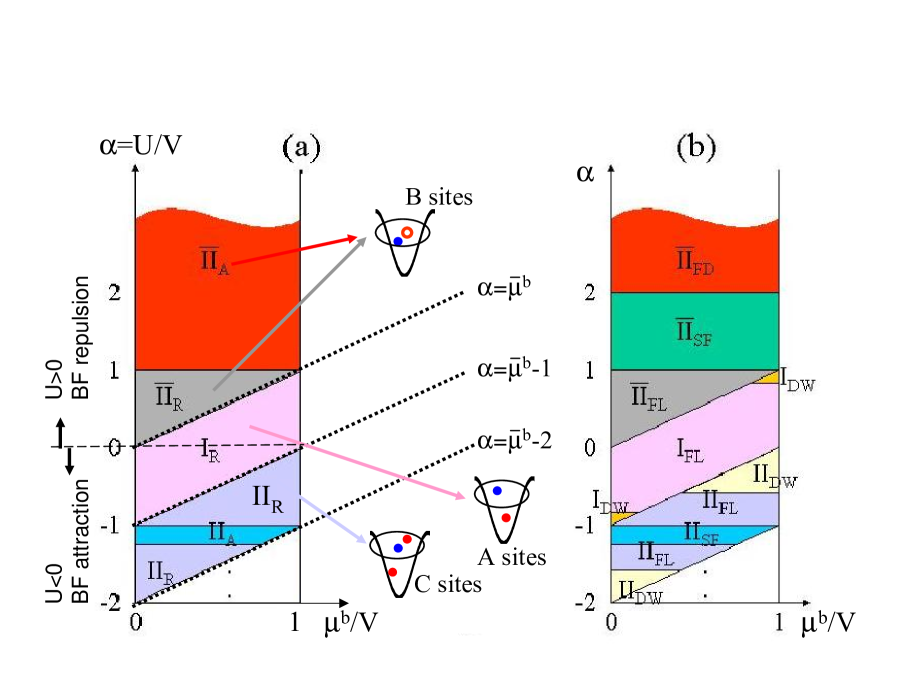
Figure 1: (color online) Quantum phase diagrams of Fermi-Bose mixtures in an homogeneous optical lattice as functions of $\tilde{\mu}^{\textrm{b}}$ and $\alpha=U/V$, for $\rho_{\textrm{f}}=0.4$ and $J/V=0.02$. (a) Diagram of composites where the filled blue (red) dots symbolize fermions (bosons) and the red empty dots, bosonic holes. (b) Detailed quantum phase diagram of fermionic composites.

In the limit of vanishing hopping ($J=0$) with finite repulsive boson-boson interaction $V$, and in the absence of interactions between bosons and fermions ($U=0$), the bosons are in a Mott insulator (MI) phase with exactly $\tilde{n}=\lceil\tilde{\mu}^{\textrm{b}}\rceil+1$ bosons per site, where $\tilde{\mu}^{\textrm{b}}=\mu^{\textrm{b}}/V$ and $\lceil x\rceil$ denotes the integer part of $x$. In contrast, the fermions can be in any set of Wannier states, since for vanishing tunneling, the energy is independent of their configuration. The situation changes when the interparticle interactions between bosons and fermions, $U$, are turned on. In the following, we define $\alpha=U/V$ and we consider the case of bosonic MI phase with $\tilde{n}$ boson per site. The presence of a fermion in site $i$ may attract $-s>0$ bosons or equivalently expel $s\leq\tilde{n}$ boson(s) depending on the sign of $U$. The on-site energy gain in attracting $-s$ bosons or expelling $s$ bosons from site $i$ is $\Delta E_{i}=\frac{V}{2}s(s-2\tilde{n}+1)-Us+\mu^{\textrm{b}}s$. Minimizing $\Delta E_{i}$ it clearly appears energetically favorable to expel $s=\left\lceil\alpha-\tilde{\mu}^{\textrm{b}}\right\rceil+\tilde{n}$ bosons. Within the occupation number basis, excitations correspond of having $\tilde{n}-s\pm 1$ boson in a site with a fermion, instead of $\tilde{n}-s$ and, therefore, the corresponding excitation energy is $\sim V$. In the following, we assume that the temperature is smaller than $V$ so that the population of the above mentioned excitations can be neglected. It follows that tunneling of a fermion is necessarily accompanied by the tunneling of $-s$ bosons (if $s<0$) or opposed-tunneling of $s$ bosons (if $s\geq 0$). The dynamics of our Fermi-Bose mixture can thus be regarded as the one of composite fermions made of one fermion plus $-s$ bosons (if $s<0$) or one fermion plus $s$ bosonic holes (if $s\geq 0$). The annihilation operators of the composite fermions are lewen :

$$F_{i} = \sqrt{\frac{(\tilde{n}-s)!}{\tilde{n}!}}\left(b_{i}^{\dagger}\right)^{s}f_{i}\quad\mbox{for $s$ bosonic holes}$$ (2)

$$F_{i} = \sqrt{\frac{\tilde{n}!}{(\tilde{n}-s)!}}\left(b_{i}\right)^{-s}f_{i}\quad\mbox{for $-s$ bosons}.$$ (3)

These operators are fermionic in the sub-Hilbert space generated by $|n-ms,m\rangle$ with $m=0,1$ in each lattice. Note that within the picture of fermionic composites, the vacuum state corresponds to MI phase with $\tilde{n}$ boson per site. At this point, different composite fermions appear depending on the values of $\alpha$, $\tilde{n}$ and $\tilde{\mu}^{\textrm{b}}$ as detailed in Fig. 1 lewen . The different composites are denoted by Roman numbers $I$, $II$, $III$, etc, which denote the total number of particles that form the corresponding composite fermion. Additionally, a bar over a Roman number indicates composite fermions formed by one bare fermion and bosonic holes, rather than bosons. For the sake of simplicity, we shall consider only bosonic MI phases with $\tilde{n}=1$ boson per site (i.e., $0<\tilde{\mu}^{\textrm{b}}\leq 1$) in the following parts of this paper foot1 .

If $\alpha-\tilde{\mu}^{\textrm{b}}>0$, a fermion in site $i$ pushes the boson out of the site. We will call the sites with this property $B$-sites. This notation will become particularly important in the presence of disorder (local $\tilde{\mu}^{\textrm{b}}$). The composites, in this case, correspond to one fermion plus one bosonic hole (this phase is called $\overline{II}$ in Fig. 1(a)). If $-1<\alpha-\tilde{\mu}^{\textrm{b}}<0$, we have bare fermions as composites (this corresponds to phase $I$). The sites with this property will be called $A$-sites. Finally, if $-2<\alpha-\tilde{\mu}^{\textrm{b}}<-1$, the composites are made of one fermion plus one boson (phase $II$). The sites with the latter property will be called $C$-sites. Because all sites are equivalent for the fermions, the ground state is highly $[N!/(N_{\textrm{f}})!(N-N_{\textrm{f}})!]$-degenerated, so the manifold of ground states is strongly coupled by fermion or boson tunneling. We assume now that the tunneling rate $J$ is small but finite. Using time-dependent degenerate perturbation theory cohen , we derive an effective Hamiltonian Auerbach for the fermionic composites:

$$H_{\textrm{eff}}=-d_{\textrm{eff}}\sum_{\langle i,j\rangle}(F^{\dagger}_{i}F_{j}+h.c.)+K_{\textrm{eff}}\sum_{\langle i,j\rangle}M_{i}M_{j}-\overline{\mu}_{\textrm{eff}}\sum_{i}M_{i}$$ (4)

where $M_{i}=F^{\dagger}_{i}F_{i}$ and $\overline{\mu}_{\textrm{eff}}$ is the chemical potential, which value is fixed by the total number of composite fermions. The nearest neighbor hopping for the composites is described by $-d_{\textrm{eff}}$ and the nearest neighbor composite-composite interactions is given by $K_{\textrm{eff}}$, which may be repulsive ($>0$) or attractive ($<0$). This effective model is equivalent to that of spinless interacting fermions. The interaction coefficient $K_{\textrm{eff}}$ originates from $2$-nd order terms in perturbative theory and can be written in the general form :

$$K_{\textrm{eff}}=\frac{-2J^{2}}{V}\left[{(2\tilde{n}-s)(\tilde{n}+1)-s(\tilde{n}-s)}-\frac{(\tilde{n}-s)(\tilde{n}+1)}{1+s-\alpha}-\frac{(\tilde{n}-s+1)\tilde{n}}{1-s+\alpha}-\frac{1}{s\alpha}\right].$$ (5)

This expression is valid in all the cases but when $s=0$, the last term ($1/s\alpha$) should not be taken into account. $d_{\textrm{eff}}$ originates from $(|s|+1)$-th order terms in perturbative theory and thus presents different forms in different regions of the phase diagram of Fig. 1. For instance in region I, $d_{\textrm{eff}}=J$, in region $\overline{II}$ $d_{\textrm{eff}}=2J^{2}/U$ and in region II, $d_{\textrm{eff}}=4J^{2}/|U|$.

The physics of the system is determined by the ratio $K_{\textrm{eff}}/d_{\textrm{eff}}$ and the sign of $K_{\textrm{eff}}$. In Fig. 1(a), the subindex A/R denotes attractive ($K_{\textrm{eff}}>0$) / repulsive ($K_{\textrm{eff}}<0$) composites interactions. Fig. 1(b) shows the quantum phase diagram of composites for fermionic filling factor $\rho_{\textrm{f}}=0.4$ and tunneling $J/V=0.02$. As an example, let us consider the case of repulsive interactions between bosons and fermions, $\alpha>0$. Once the fermion-bosonic hole composites $\overline{II}$ have been created ($\alpha>\tilde{\mu}^{\textrm{b}}$), the relation $K_{\textrm{eff}}/d_{\textrm{eff}}=-2(\alpha-1)$ applies. Consequently, if one increases the interactions between bosons and fermions adiabatically, the system evolves through different quantum phases. For $\tilde{\mu}^{\textrm{b}}<\alpha<1$, the interactions between composite fermions are repulsive and of the same order of the tunneling; the system exhibits delocalized metallic phases. For $\alpha\simeq 1$, the interactions between composite fermions vanish and the system show up the properties of an ideal Fermi gas. Growing further the repulsive interactions between bosons and fermions, the interactions between composite fermions become attractive. For $1<\alpha<2$, one expects the system to show superfluidity, and for $\alpha>2$ fermionic insulator domains are predicted.

In the reminder of the paper, we shall generalize these results to the case of inhomogeneous optical lattices. We shall assume diagonal inhomogeneities, i.e., site-dependent local energies ($\mu_{i}^{\textrm{b,f}}$ depends on site $i$ but the tunneling rate $J$ and interactions $U$ and $V$ do not). Diagonal inhomogeneities may account for (i) overall trapping potential (usually harmonic), which is usually underlying in experiments on ultracold atoms, and (ii) disorder that may be introduced in different ways in ultracold samples (see section VI for details).

III.2 Composites in disordered lattices: effective Hamiltonian

In this section we include on-site energy inhomogeneities in the optical lattice and we derive a generalized effective Hamiltonian for the composite fermions. Strictly speaking, in the presence of disorder the hopping terms should depend on the site under consideration. Nevertheless, for weak enough disorder one can assume site independent tunneling for both bosons or fermions boseglass . In the following we will restrict ourselves to the case where the hopping rates of bosons and fermions are equal and site-independent, $J_{b}=J_{f}=J$ and to the strong coupling regime, $V,U>>J$, where the tunneling can be considered as a perturbation, as in section III.1.

For homogeneous lattices (see section III.1), following the lines of Refs. svistunov ; lewen , we have used the method of degenerate second order perturbation theory to derive the effective Hamiltonian (4) by projecting the wave function onto the multiply degenerated ground state of the system in the absence of tunneling.

In the inhomogeneous case, this approach cannot be applied since even for $J=0$ there exists a well defined single ground state determined by the values of the local chemical potentials. Nevertheless, in general, there will be a manifold of many states with similar energies. The differences of energy inside a manifold are of the order of the difference of chemical potential in different sites, whose random distribution is bounded, i.e., $0\leq\tilde{\mu}^{\textrm{b}}_{i}$, $\tilde{\mu}^{\textrm{f}}_{i}\leq 1$. Moreover, the lower energy manifold is separated from the exited states by a gap given by the boson-boson interaction, $V$. Therefore, one can apply a form of quasidegenerate perturbation theory by projecting onto the manifold of near-ground states cohen .

As it is described in Refs. cohen and briefly summarized in Appendix A, we construct an effective Hamiltonian that describes the slow, low-energy perturbation induced within the manifold of unperturbed ground states by means of a unitary transformation applied to the total Hamiltonian (III). By denoting with P the projector on the manifold and Q=1-P its complement, the expression of the effective Hamiltonian can be written as:

$$\langle out|H_{\textrm{eff}}|in\rangle=\langle out|H_{0}|in\rangle+\langle out|PH_{int}P|in\rangle$$ (6)

$$-\frac{1}{2}\langle out|PH_{int}Q\left(\frac{1}{H_{0}-E_{in}}+\frac{1}{H_{0}-E_{out}}\right)QH_{int}P|in\rangle.$$

As second order theory can only connect states that differ on one set of two adjacent sites, the effective Hamiltonian $H_{\textrm{eff}}$ can only contain nearest-neighbor hopping and interactions as well as on-site energies $\overline{\mu}_{i}$ anna :

$$H_{\textrm{eff}}=\sum_{\langle i,j\rangle}\left[-d_{i,j}F^{\dagger}_{i}F_{j}+h.c.\right]+\sum_{\langle i,j\rangle}K_{i,j}M_{i}M_{j}+\sum_{i}\overline{\mu}_{i}M_{i}$$ (7)

where $M_{i}$, $F_{i}$ are defined as in (4). The explicit calculation of the coefficients $d_{i,j}$, $K_{i,j}$ and $\overline{\mu}_{i}$ depends on the concrete type of composites. In the three following sections we address the cases of fermion-bosonic hole composites ($\overline{II}$), bare fermion composites ($I$), and fermion-boson composites ($II$).

III.3 Fermion-Bosonic hole composites

In this section, we assume that all sites are $B$-sites, i.e., $\alpha-\tilde{\mu}_{i}^{\textrm{b}}>0$, so that composite fermions $\overline{II}$ are created. This means that each site contains either one boson or one fermion plus a bosonic hole. Thus, the manifold of low lying states comprises all possible configurations of $N_{\textrm{f}}$ fermions on an $N$-site lattice, with no fermion occupied sites filled by bosons.

Within the manifold of ground states, a fermion jump from site $i$ to site $j$ can only occur if the boson that was initially in site $j$ jumps back to site $i$ into the hole the fermion leaves behind. Therefore, the number operator for fermions and bosons are related with the number operator of composites, i.e., $M_{i}=m_{i}=1-n_{i}$. Note that the composite model is expressed in terms of the composite fermionic operators $F_{i}=b^{\dagger}_{i}f_{i}$ and thus $M_{i}=f^{\dagger}_{i}f_{i}b_{i}b^{\dagger}_{i}$. To determine the coefficients in (7), one looks at two adjacent sites with indices $i$ and $j$ and uses a vector notation $|1_{\textrm{b}},1_{\textrm{f}}\rangle$ which would correspond to one boson on site $i$ and one fermion on site $j$. In the composite fermion picture this would be denoted as $|0,1\rangle^{c}$, i.e., one composite fermion on site $j$ and no composite fermion on site $i$. With this notation tunneling rates and nearest neighbor-interactions are calculated from Eq. (6) as:

$$\langle 1_{\textrm{f}},1_{\textrm{b}}|H_{eff}|1_{\textrm{b}},1_{\textrm{f}}\rangle = -\frac{1}{2}\frac{J^{2}}{V}\left(\frac{1}{\alpha-\Delta_{ij}^{\textrm{b}}}+\frac{1}{\alpha+\Delta_{ij}^{\textrm{b}}}+\frac{1}{\alpha-\Delta_{ij}^{\textrm{f}}}+\frac{1}{\alpha+\Delta_{ij}^{\textrm{f}}}\right)$$ (8)

$$\equiv {}^{c}\langle 1,0|F^{\dagger}_{i}F_{j}|0,1\rangle^{c}$$

$$\langle 1_{\textrm{b}},1_{\textrm{b}}|H_{eff}|1_{\textrm{b}},1_{\textrm{b}}\rangle = -\frac{1}{2}\frac{J^{2}}{V}\left(\frac{2}{1-\Delta_{ij}^{\textrm{b}}}+\frac{2}{1+\Delta_{ij}^{\textrm{b}}}+\frac{2}{1-\Delta_{ij}^{\textrm{b}}}+\frac{2}{1+\Delta_{ij}^{\textrm{b}}}\right)$$ (9)

$$\equiv {}^{c}\langle 0,0|(1-M_{i})(1-M_{j})|0,0\rangle^{c}$$

$$\langle 1_{\textrm{f}},1_{\textrm{b}}|H_{eff}|1_{\textrm{f}},1_{\textrm{b}}\rangle = -\frac{1}{2}\frac{J^{2}}{V}\left(\frac{2}{\alpha-\Delta_{ij}^{\textrm{b}}}+\frac{2}{\alpha+\Delta_{ij}^{\textrm{f}}}\right)$$ (10)

$$\equiv {}^{c}\langle 1,0|M_{i}(1-M_{j})|1,0\rangle^{c}$$

$$\langle 1_{\textrm{b}},1_{\textrm{f}}|H_{eff}|1_{\textrm{b}},1_{\textrm{f}}\rangle = -\frac{1}{2}\frac{J^{2}}{V}\left(\frac{1}{\alpha+\Delta_{ij}^{\textrm{b}}}+\frac{1}{\alpha-\Delta_{ij}^{\textrm{f}}}\right)$$ (11)

$$\equiv {}^{c}\langle 1,0|M_{i}(1-M_{j})|1,0\rangle^{c}$$

Summing these terms up yields the coefficients for (7):

$$d_{ij} = \frac{J^{2}}{V}\left(\frac{\alpha}{\alpha^{2}-(\Delta^{\textrm{b}}_{ij})^{2}}+\frac{\alpha}{\alpha^{2}-(\Delta^{\textrm{f}}_{ij})^{2}}\right)$$ (12)

$$K_{ij} = -\frac{J^{2}}{V}\Bigg{(}\frac{4}{1-(\Delta^{\textrm{b}}_{ij})^{2}}-\frac{2\alpha}{\alpha^{2}-(\Delta^{\textrm{f}}_{ij})^{2}}-\frac{2\alpha}{\alpha^{2}-(\Delta^{\textrm{b}}_{ij})^{2}}\Bigg{)}$$ (13)

$$\overline{\mu}_{i} = \mu_{i}^{\textrm{b}}-\mu_{i}^{\textrm{f}}+\frac{J^{2}}{V}\left[\sum_{\langle i,j\rangle}{\frac{4}{1-(\Delta_{ij}^{\textrm{b}})^{2}}}-{\frac{1}{\alpha-\Delta_{ij}^{\textrm{b}}}}-{\frac{1}{\alpha+\Delta_{ij}^{\textrm{f}}}}\right]$$ (14)

with $\Delta_{ij}^{\textrm{f,b}}=\tilde{\mu}_{i}^{\textrm{f,b}}-\tilde{\mu}_{j}^{\textrm{f,b}}$. Here, $\langle i,j\rangle$ represents all neighbor sites of $i$. We shall now consider separately two limiting cases: (i) $\mu_{i}^{\textrm{f}}=0$ and $\mu_{i}^{\textrm{b}}=\mu_{i}V$, and (ii) $\mu_{i}^{\textrm{f}}=\mu_{i}^{\textrm{b}}=\mu_{i}V$ .

III.3.1 Case where $\mu_{i}^{\textrm{f}}=0$

In the first case, we assume that the on-site energy for fermions vanishes. We assume also that all sites are $B$-sites, i.e., $\alpha-\tilde{\mu}_{i}^{\textrm{b}}>0$ everywhere. In this case, the hopping amplitudes $d_{ij}$ are always positive, although may vary quite significantly with disorder, especially when $\Delta_{ij}^{\textrm{b}}\simeq\alpha$. As shown in Fig. 2, for $\alpha>1$, $K_{ij}\leq 0$ and we deal with attractive (although random) interactions. For $\alpha<1$, $K_{ij}\geq 0$ and the interactions between composites are repulsive. For $\alpha<1$, but close to 1, $K_{ij}$ might take positive or negative values for $\Delta_{ij}^{\textrm{b}}$ small or $\Delta_{ij}^{\textrm{b}}\simeq\alpha$. In this case, the qualitative character of interactions may be controlled by inhomogeneity anna . At low temperatures the physics of the system will depend on the relation between $\tilde{\mu}_{i}^{\textrm{b}}$’s and $\alpha$.

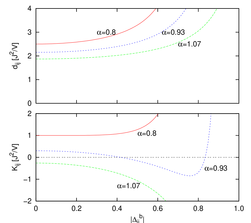
Figure 2: Tunneling, $d_{ij}$, and nearest neighbor couplings, $K_{ij}$, of type $\overline{II}$ composites as a function of disorder $\Delta_{ij}^{\textrm{b}}$, and for different boson-fermion interactions, $\alpha$, in the case $\mu_{i}^{\textrm{f}}=0$.

Small disorder limit -

For small disorder, we may neglect the contributions of $\Delta_{ij}^{\textrm{b}}$ to $d_{ij}\simeq d$ and $K_{ij}\simeq K$, and keep only the leading disorder contribution in $\overline{\mu}_{i}$, i.e., the first term in Eq. (14). Note, that the latter contribution is relevant in 1D and 2D leading to Anderson localization of single particles gang . When $K/d\ll 1$ the system will then be in the Fermi glass phase, i.e., Anderson localized (and many-body corrected) single particle states will be occupied according to the Fermi-Dirac rules fermiglass . For repulsive interactions and $K/d\gg 1$, the ground state will be a Mott insulator and the composite fermions will be pinned for large filling factors. In particular, for filling factor $\rho_{\textrm{f}}=1/2$, one expects the ground state to be in the form of a checker-board. For intermediate values of $K/d$, with $K>0$, delocalized metallic phases with enhanced persistent currents are possible metalglass . Similarly, for attractive interactions ($K<0$) and $|K|/d<1$ one expects competition between pairing of fermions and disorder, i.e., a ”dirty” superfluid phase while for $|K|/d\gg 1$, the fermions will form a domain insulator. Fig. 3 shows a schematic representation of expected disordered phases of the type $\overline{II}$ fermionic composites for small disorder, and vanishing fermionic on-site chemical potential.

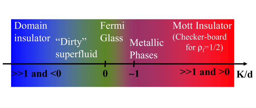
Figure 3: (color online) Schematic phase diagram of type $\overline{II}$ fermionic composites for low disorder ($\Delta_{ij}^{\textrm{b}}\ll 1,\alpha$) and vanishing fermionic on-site energy ($\mu_{i}^{\textrm{f}}=0$) as a function of the ratio between n.n. interactions and tunneling for the composites.

Spinglass limit -

Another interesting limit corresponds to the case $\Delta_{ij}^{\textrm{b}}\simeq\alpha\simeq 1$. Such a situation can be achieved by combining a superlattice potential with a spatial period twice as large as the one of the lattice (which alone induces $|\Delta_{ij}^{\textrm{b}}|=1$) and a random potential to induce site-to-site fluctuations. The tunneling becomes then non-resonant and can be neglected in Eq. (7), while the couplings $K_{ij}$ fluctuate strongly as shown in Fig. 2. We end up then with the (fermionic) Ising spin glass model anna described by the Edwards-Anderson model with $s_{i}=2M_{i}-1=\pm 1$. This case is studied in more detail in section V.

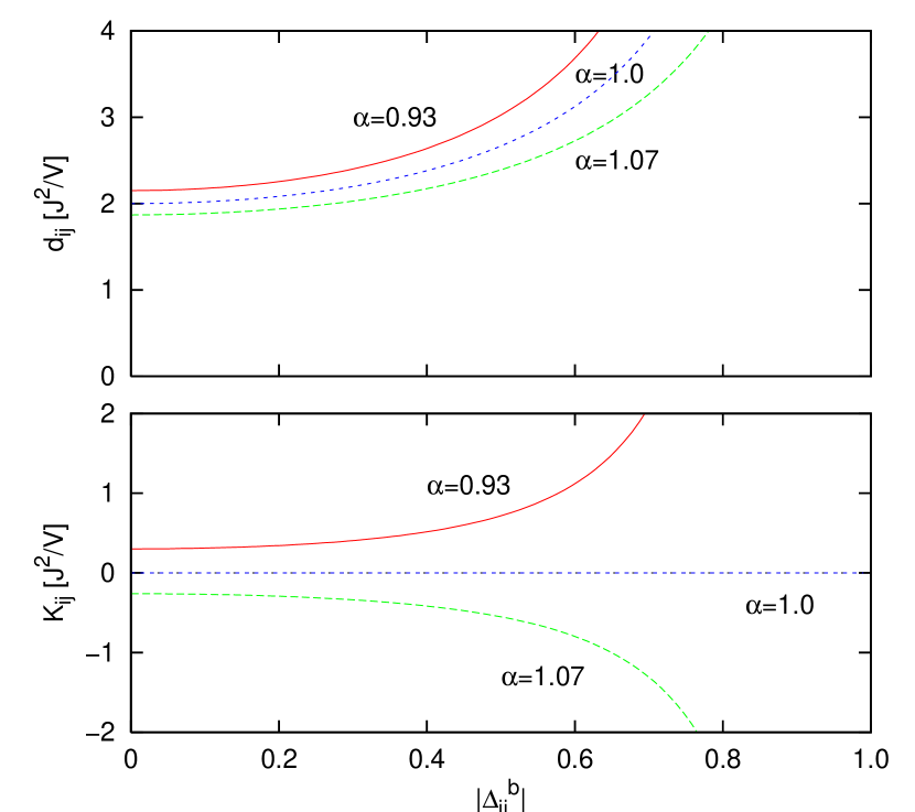
Figure 4: Tunneling, $d_{ij}$, and nearest neighbor couplings, $K_{ij}$, of type $\overline{II}$ composites as a function of disorder $\Delta_{ij}^{\textrm{b}}$, and for different boson-fermion interactions, $\alpha$, in the case $\mu_{i}^{\textrm{f}}=\mu_{i}^{\textrm{b}}=\mu_{i}V$.

III.3.2 Case where $\mu_{i}^{\textrm{f}}=\mu_{i}^{\textrm{b}}$

Let us now consider that the chemical potential is equal for bosons and fermions at each lattice site, $\mu_{i}^{\textrm{f}}=\mu_{i}^{\textrm{b}}=\mu_{i}V$. All sites are still assumed to be $B$-sites.

The effective interactions are for $\alpha>1$ always negative, and therefore the composites experience random attractive interactions (as in the previous case), while for $\alpha<1$, $K_{ij}>0$, and therefore we deal with random repulsive interactions. For $\alpha=1$, the interactions between composites vanish for all the values of the amplitude of the disorder.

In this case the sign of the interactions between composites is governed by the interactions between bosons and fermions alone. Note that this is not possible, when one considers only disorder for the bosons. Fig. 4 shows the tunneling and the nearest neighbor couplings for different values of $\alpha$. We expect here the appearance of similar phases, as in the previously discussed case.

III.4 Bare Fermion composites

In this section we now assume that all sites are $A$-sites and correspond to type $I$ fermionic composites, i.e., $-1<\alpha-\tilde{\mu}^{\textrm{b}}_{i}<0$. This means that composite fermions reduce to bare fermions ($F_{i}=f_{i}$) flowing on the top of a MI phase with $\tilde{n}=1$ boson per site. Each site contains now one boson plus eventually one fermion. From application of perturbation theory as described in section III.2 [see Eq. (6)], one finds that the coefficients of the effective Hamiltonian (7) are:

$$d_{ij} = J,$$ (15)

$$K_{ij} = -\frac{J^{2}}{V}\left(\frac{8}{1-(\Delta^{\textrm{b}}_{ij})^{2}}-\frac{4(1+\alpha)}{(1+\alpha)^{2}-(\Delta^{\textrm{b}}_{ij})^{2}}-\frac{4(1-\alpha)}{(1-\alpha)^{2}-(\Delta^{\textrm{b}}_{ij})^{2}}\right),$$ (16)

$$\overline{\mu}_{i} = -\mu_{i}^{\textrm{f}}+\frac{J^{2}}{V}\sum_{\langle i,j\rangle}\left[{\frac{4}{1-(\Delta_{ij}^{\textrm{b}})^{2}}}-{\frac{1}{\Delta_{ij}^{\textrm{f}}}}-{\frac{4}{1-(\alpha-\Delta_{ij}^{\textrm{b}})^{2}}}\right]~{}.$$ (17)

We observe that the inhomogeneities for fermions (site-dependent $\mu_{i}^{\textrm{f}}$) do not neither perturb the effective tunneling, nor the effective interaction parameter, while $\overline{\mu}_{i}\simeq-\mu_{i}^{\textrm{f}}$ up to corrections of the order of $\textrm{O}(J^{2}/V)$ for type I composite (bare) fermions. In this case, composite tunneling $d_{ij}$ originates from the first order term, while the nearest neighbor interaction originates from second order perturbation. It should be noted that in the case of type $I$ composites, the hopping $d_{ij}$ and interaction $K_{ij}$ parameters in Eq. (7) do not depend on the sign of the fermion-boson interaction $\alpha$.

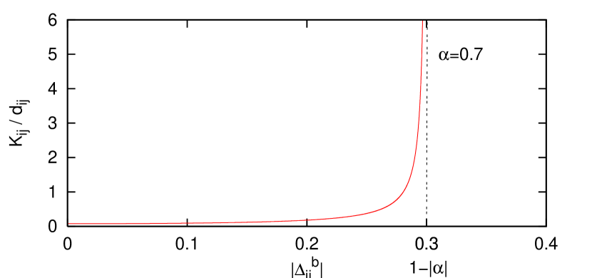
Figure 5: Ratio of nearest neighbor coupling and tunneling $K_{ij}/d_{ij}$ as a function of disorder $\Delta_{ij}^{\textrm{b}}$ for $\alpha=0.7$ and $J/V=0.01$ in the case of type $I$ composite fermions.

The couplings $K_{ij}$ are always positive, and for $\alpha\simeq 0$, $K_{ij}\simeq\textrm{O}(\alpha^{2})$, and both the repulsive interactions, and disorder are very weak, leading to an almost ideal Fermi liquid behavior at low temperature. For finite $\alpha$, and $\Delta_{ij}^{\textrm{b}}\simeq 1-|\alpha|$, however, the fluctuations of $K_{ij}$ might be quite large as shown in Fig. 5. Note, that for $|\alpha|\simeq 1$, this will occur even for small disorder. It is interesting to note that the dynamics of type $I$ composites in our system resembles quantum bond percolation. As suggested from Fig. 5, one can assume in a somehow simplified view that the interaction parameter $K_{ij}$ takes either very large, or zero values. The lattice decomposes into two sub-lattices (see Fig. 6): a ”weak” bond sub-lattice (corresponding to $K_{ij}\ll d_{ij}$) in which fermions flow as in an almost ideal Fermi liquid, and a ”strong” sub-lattice (corresponding to $K_{ij}\gg d_{ij}$), where only one fermion per bond is allowed ($M_{i}M_{j}=0$ for all nearest neighbors in the ”strong” cluster). Therefore, we see that the physics of bond percolation percbook ; grimmett will play a role. For $p>p_{\textrm{c}}$, where $p$ is the density of weak bonds and $p_{\textrm{c}}\simeq 0.50$ (in two-dimensional square lattices) and $p_{\textrm{c}}\simeq 0.25$ (in three-dimensional cubic lattices), the weak bond sub-lattice will be percolating, i.e., there exists a large cluster of weak bonds which spans the lattice from one side to the other. The question arises as to determine the quantum bond percolation threshold $p_{\textrm{Q}}$, i.e., for which minimal value of $p$, the eigenstates of the quantum gas will be delocalized over the extension of the system. Although it is clear that $p_{\textrm{Q}}>p_{\textrm{c}}$, it is still an open question to determine the exact value for the quantum percolation threshold $p_{\textrm{Q}}$ shapir ; chang ; root ; soukoulis91 ; soukoulis92 . Therefore, experimental realization of our system may be of considerable interest for addressing this general question.

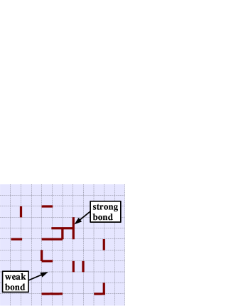
Figure 6: Schematic representation of connecting bonds in type $I$ composite systems. The bonds are separated in two types: (i) the weak bonds in which two composites do not interact and (ii) the strong bonds where only one composite can stay. The short lines represent the bonds and the crossing points of the bonds are the lattice sites.

III.5 Fermion-Boson composites

We finally consider in this section the case, when all sites are $C$-sites, so that type II composites corresponding to $-2<\alpha-\tilde{\mu}_{i}^{\textrm{b}}<-1$ are formed. The composites are made of one fermion and one boson. This means that each lattice site is populated by either one boson or one fermion plus two bosons. Tunneling as well as nearest neighbor interaction of composites arise from 2nd order terms in perturbative theory [see section III.2 and Eq. (6) for details]. Along the lines of section III.2, we find the following expressions:

$$d_{ij} = \frac{J^{2}}{V}\left(\frac{2|\alpha|}{|\alpha|^{2}-(\Delta^{\textrm{b}}_{ij})^{2}}+\frac{2|\alpha|}{|\alpha|^{2}-(\Delta^{\textrm{f}}_{ij})^{2}}\right),$$ (18)

$$K_{ij} = \frac{-J^{2}}{V}\left(\frac{16}{1-(\Delta_{ij}^{\textrm{b}})^{2}}-\frac{2|\alpha|}{|\alpha|^{2}-{(\Delta_{ij}^{\textrm{f}})}^{2}}-\frac{8|\alpha|}{|\alpha|^{2}-{(\Delta_{ij}^{\textrm{b}})}^{2}}-\frac{6(2-|\alpha|)}{(2-|\alpha|)^{2}-{(\Delta_{ij}^{\textrm{b}})}^{2}}\right),$$ (19)

$$\overline{\mu}_{i} = -\mu_{i}^{\textrm{f}}-\mu_{i}^{\textrm{b}}+\frac{J^{2}}{V}\sum_{\langle i,j\rangle}\left[{\frac{4}{1-(\Delta_{ij}^{\textrm{b}})^{2}}}-{\frac{4}{|\alpha|+\Delta_{ij}^{\textrm{b}}}}-{\frac{3}{2-|\alpha|-\Delta_{ij}^{\textrm{b}}}}-{\frac{1}{|\alpha|+\Delta_{ij}^{\textrm{f}}}}\right]~{}.$$ (20)

Different scenarios also arise in this case. In the following, we shall consider the case $\mu_{i}^{\textrm{f}}=0$ and $\mu_{i}^{\textrm{b}}=\mu_{i}V$. The other extreme case, $\mu_{i}^{\textrm{f}}=\mu_{i}^{\textrm{b}}=\mu_{i}V$, leads to qualitatively similar conclusions.

III.5.1 Case where $\mu_{i}^{\textrm{f}}=0$

We assume here that the on-site energy for fermions is $\mu_{i}^{\textrm{f}}=0$. As for Fig. 2, we plot the effective tunneling and interaction parameter versus inhomogeneity parameter $\Delta_{ij}^{\textrm{b}}$ in Fig. 7. The general behavior of $d_{ij}$ and $K_{ij}$ is qualitatively the same as in the case of type $\overline{II}$ composites. For type $II$ composites, and for small disorder, we find $K/d=1-4|\alpha|+3/(2-|\alpha|)$ with $1<|\alpha|<2$. The inhomogeneity is now given, for type $II$ composites, by $\overline{\mu}_{i}=-\mu_{i}^{\textrm{b}}$. The regimes, where $K\ll d$ corresponding to an almost ideal Fermi gas (in the absence of disorder), or to a Fermi glass (in the presence of disorder), can be reached in the region $\alpha\simeq-5/4$. The opposite regimes of strong effective interactions, where $K\gg d$ appears for $\alpha\gtrsim-2$, and corresponds to repulsive interactions $K>0$. In this region, the fermionic checkerboard phase if the filling factor is $1/2$ (for vanishing disorder) and the repulsive Fermi glass phase (in the presence of disorder) are expected. Here, no strong attractive interactions regime occurs since $K/d$ reaches a minimum of $\simeq-0.07$ for $\alpha=\sqrt{3}/2-2$. Therefore, in contrast to type $\overline{II}$ composites, for type ${II}$ composites: (i) due to weakness of attractive interactions, the domain insulator phase does not appear, and even the ”dirty” superfluid phase may be washed out; and (ii) arbitrary strong repulsive interactions can be used to generate a Mott insulator, which might be difficult for $\overline{II}$ composites, where $K/d$ is limited to $2$, suggesting that Fermi liquid, Fermi glass behavior will prevail.

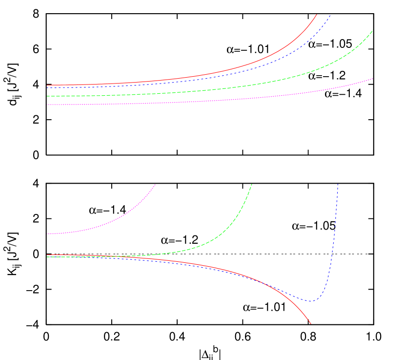
Figure 7: Tunneling, $d_{ij}$, and nearest neighbor couplings, $K_{ij}$, of type ${II}$ composites as a function of disorder $\Delta_{ij}^{\textrm{b}}$ and for different boson-fermion interactions, $\alpha$, in the case $\mu_{i}^{\textrm{f}}=0$.

As shown in Fig. 7, the spinglass limit can also be reached for example for $\alpha\simeq-1.05$ and $|\Delta_{ij}^{\textrm{f}}|\simeq 0.9$. In this regime, the tunneling is non-resonant due to strong disorder and the nearest neighbor interaction fluctuates strongly from negative to positive values. See section V for further study of the spinglass limit.

III.6 Optical lattices with different types of sites

III.6.1 Sites A and B

Obviously, the situation becomes much more complex when we deal with different types of sites in the lattice. Again there are infinitely many possibilities, and the simplest ones are, for instance: i) coexistence of $A$- and $B$-sites, or ii) $A$- and $C$- sites, or iii) $A$-, $B$-, and $C$-sites, etc. In the following we shall consider only the case i) with $\mu_{i}^{\textrm{f}}=0$ and $\mu_{i}^{\textrm{b}}=\mu_{i}V$, since the other cases lead to qualitatively similar effects.

Let us assume that the numbers of $A$-, and $B$- sites are macroscopic, i.e., of the order of $N$. More precisely, we will consider that $N_{A}$ (number of $A$-sites) and $N_{B}$ (number of $B$-sites) of order N/2. In this case the physics of site percolation percbook will play a role. If $N_{\textrm{f}}\leq N_{B}$ the composite fermions will move within a cluster of $B$-sites. When $N_{B}$ will be above the classical percolation threshold, this cluster will be percolating. The expressions Eq. (12) and Eq. (13) will still be valid, except that they will connect only the $B$-sites. The physics of the system will be similar as in the case of type $I$ composites), but it will occur now on the percolating cluster. For small disorder, and $K/d\ll 1$ the system will be in a Fermi glass phase in which the interplay between the Anderson localization of single particles due to fluctuations of $\mu_{i}^{\textrm{b}}$ and quantum percolation effects, that is randomness of the $B$-sites cluster, will occur. For repulsive interactions and $K/d\gg 1$, the ground state will be a Mott insulator on the cluster and the composite fermions will be pinned (in particular for half-filling of the cluster). It is an open question whether the delocalized metallic phases with enhanced persistent current of the kind discussed in Ref. metalglass might exist in this case. Similarly, it is an open question whether for attractive interactions ($K<0$) and $|K|/d<1$ pairing of (perhaps localized) fermions will take place. In the case of $|K|/d\gg 1$, we expect that the fermions will form a domain insulator on the cluster.

In the ”spin-glass” limit $\Delta_{ij}^{\textrm{b}}\simeq\alpha\simeq 1$, we will deal with the Edward-Anderson spin glass on the cluster. Such systems are of interest in condensed matter physics (cf. spiperc ), and again questions connected to the nature of spin glass ordering may be studied in this case.

When $N_{\textrm{f}}>N_{B}$, all $B$-sites will be filled, and the physics will occur on the cluster of $A$-sites. For $\alpha\simeq 0$, we will deal with a gas with very weak repulsive interactions, and no significant disorder on the random cluster; this is an ideal test to study quantum percolation at low T. For finite $\alpha$, and $\Delta_{ij}^{\textrm{b}}\simeq 1-\alpha$, the interplay between the fluctuating repulsive $K_{ij}$’s and quantum percolation might be studied.

IV Numerical analysis using Gutzwiller ansatz

IV.1 Numerical method

In this section, we present numerical results that give evidences of (i) formation of composite particles in Fermi-Bose mixtures in optical lattices and (ii) existence of different quantum phases for various sets of composite tunneling and interaction parameters and inhomogeneities. We mainly focus on type $\overline{II}$ composites. Mean field theory provides appropriate although not exact properties of Hubbard models sachdev . In the following, we consider a variational mean field approach provided by the Gutzwiller ansatz (GA) fisher ; statGA . In particular, the GA ansatz has been successfully employed for bosonic systems to study the superfluid to Mott Insulator transition fisher ; jaksch in non-disordered lattices, and the Anderson and Bose glass transitions in the presence of disorder fisher ; boseglass .

Briefly, the Gutzwiller approach neglects site-to-site quantum coherences so that the many-body ground state is written as a product of $N$ states, each one being localized in a different lattice site. Each localized state is a superposition of different Fock states $|n,m\rangle_{i}$ with exactly $n$ bosons and $m$ fermions on the $i$-th lattice site :

$$|\psi_{\textrm{MF}}\rangle=\prod_{i=1}^{N}\left(\sum_{n=0}^{n_{\textrm{max}}}\sum_{m=0,1}g^{(i)}_{n,m}|n,m\rangle_{i}\right)$$ (21)

where $n_{\textrm{max}}$ is an arbitrary maximum occupation number of bosons in each lattice site foot2 .

The $g^{(i)}_{n,m}$ are complex coefficients proportional to the amplitude of finding $n$ bosons and $m$ fermions in the $i$-th lattice site, and consequently we can impose, without loss of generality, these coefficients to satisfy $\sum_{n,m}|g^{(i)}_{n,m}|^{2}=1$. For the sake of simplicity, we neglect the anticommutation relation of fermionic creation ($f_{i}$) and annihilation ($f_{j}^{\dagger}$) operators in different lattice sites. However Pauli principle applies in each lattice site ($m_{i}\leq 1$ $\forall i$). Since GA neglects correlations between different sites, this procedure is expected to be safe and is commonly used within the Gutzwiller approach fb .

Inserting $|\psi_{\textrm{MF}}\rangle$ in the Schrödinger equation with the two-species Fermi-Bose Hamiltonian (III), we were able to determine the ground state and to compute the dynamical evolution of the Fermi-Bose mixture.

Ground state calculations -

Employing a standard conjugate-gradient downhill method recipes , we minimize the total energy $\langle\psi_{MF}|H_{\textrm{FBH}}|\psi_{MF}\rangle$ with $H_{FBH}$ given by (1) under the constraint of fixed total numbers of fermions $N_{\textrm{f}}$ and bosons $N_{\textrm{b}}$ foot3 :

$$\langle\psi_{\textrm{MF}}|H_{\textrm{FBH}}|\psi_{\textrm{MF}}\rangle-\Lambda_{\textrm{f}}\left(\langle\psi_{\textrm{MF}}|\sum_{i}m_{i}|\psi_{\textrm{MF}}\rangle-N_{\textrm{f}}\right)^{2}-\Lambda_{\textrm{b}}\left(\langle\psi_{\textrm{MF}}|\sum_{i}n_{i}|\psi_{\textrm{MF}}\rangle-N_{\textrm{b}}\right)^{2}~{}\rightarrow~{}\textrm{min}~{}.$$ (22)

The numerical procedure is as follows: (i) We minimize the energy of the mixture (eventually) in presence of smooth trapping potentials and with non-zero tunneling for bosons and fermions, but assuming vanishing interactions between bosons and fermions ($U=0$). During the minimization the normalization ($\sum_{n}\sum_{m}|g_{n,m}|^{2}=1$) should be imposed. (ii) After this initial minimization, we ramp up adiabatically the interactions between bosons and fermions using the dynamical Gutzwiller approach (see below). In this way, we end up with the ground state of the mixture in presence of tunneling $J$, non-vanishing interactions $U$ and $V$ and eventually in the the presence of a smooth trapping potential.

This two-step procedure is indeed necessary because in the presence of interactions between bosons and fermions finite numbers of bosons and fermions correspond to a saddle point of Eq. (22), and no true minimum can be found within direct minimization of the total Hamiltonian fboptexp .

Time-dependent calculations -

Using the time-dependent variational principle ($\langle\psi_{\textrm{MF}}|i\hbar\partial_{t}-H_{\textrm{FBH}}(t)|\psi_{\textrm{MF}}\rangle\rightarrow\textrm{min}$) with Hamiltonian $H_{BFH}$ given by (III) and eventually time-dependent parameters $J_{\textrm{f,b}}$, $U$, $V$, $\mu_{i}^{\textrm{f,b}}$, we end up with the following dynamical equation for the Gutzwiller coefficients dynamGA ; fboptexp  :

$$i\hbar\partial_{t}g^{(i)}_{n,m} = \left[\frac{V}{2}n(n-1)+Unm-\mu_{i}^{\textrm{b}}n-\mu_{i}^{\textrm{f}}m\right]g_{n,m}^{(i)}$$ (23)

$$-\left(\Sigma_{i}^{\textrm{b}}\right)\sqrt{n}\ g_{n-1,m}^{(i)}-\left(\Sigma_{i}^{\textrm{b}}\right)^{*}\sqrt{n+1}\ g_{n+1,m}^{(i)}$$

$$-\left(\Sigma_{i}^{\textrm{f}}\right)g_{n,m-1}^{(i)}-\left(\Sigma_{i}^{\textrm{f}}\right)^{*}g_{n,m+1}^{(i)}$$

where

$$\Sigma_{i}^{\textrm{b}} = \sum_{\langle i,j\rangle}{J_{\textrm{b}}\left[\sum_{n}\sum_{m=0,1}{\sqrt{n+1}\ g_{n,m}^{(j)*}\ g_{n+1,m}^{(j)}}\right]}$$ (24)

$$\Sigma_{i}^{\textrm{f}} = \sum_{\langle i,j\rangle}{J_{\textrm{f}}\left[\sum_{n}{g_{n,0}^{(j)*}\ g_{n,1}^{(j)}}\right].}$$ (25)

Note that these equations are valid under the hypothesis of neglecting anticommutation relations for fermionic operators in different sites. Equations (23-25) preserve both normalization of the wave function and the mean particle numbers.

In the following, dynamical Gutzwiller approach will be used for (i) computing the ground state of the mixture in the presence of interactions between bosons and fermions (see above) and (ii) to ramp up adiabatically disorder in the optical lattice potential.

IV.2 Numerical results

We have considered a 2D optical lattice with $N=10\times 10$ sites to perform the simulations of the different quantum phases that appear for type $\overline{II}$ composites in the presence of a very shallow harmonic trapping potential ($\mu_{i}^{\textrm{b,f}}=\omega^{\textrm{b,f}}\times l(i)^{2}$, where $l(i)$ is the distance from site $i$ to the central site in cell size units), with different amplitudes for bosons and fermions. The harmonic on-site energy simulates shallow magnetic or optical trapping. The confining potential is experimentally of vital importance in order to see Mott insulator phases, that require commensurate filling bloch ; esslinger ; phillips . It plays the role of a local chemical potential, and it has been predicted that it modifies some properties of strongly correlated phases fillingfactor . Additionally, this breaks the equivalence of all lattice sites and makes it more obvious the different phases that one can achieve (see below). We first calculate the ground state of the system considering $N_{\textrm{b}}=60$ bosons, $N_{\textrm{f}}=40$ fermions, $J_{\textrm{b}}/V=J_{\textrm{f}}/V=0.02$, $U=0$ in the presence of harmonic traps characterized by $\omega^{\textrm{b}}=10^{-7}$ and $\omega^{\textrm{f}}=5\times 10^{-7}$.

Under these conditions, we find that, as expected, the bosons are well inside the MI phase with $\tilde{n}=1$ boson per site fisher ; jaksch . Due to the very small values of $\omega^{\textrm{f}}$ and $\omega^{\textrm{b}}$ neither the bosons nor the fermions feel significantly the confining trap as shown in Fig. 8(a).

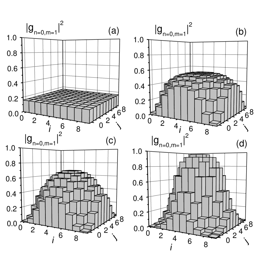
Figure 8: Probability of having one fermion and zero boson at each lattice site for the $N=100$ sites in a Fermi-Bose mixture with $N_{\textrm{b}}=60$, $N_{\textrm{f}}=40$, $J_{\textrm{b}}/V=J_{\textrm{f}}/V=0.02$ and in the presence of harmonic traps for bosons and fermions characterized by $\omega_{\textrm{b}}=10^{-7}$ and $\omega_{\textrm{f}}=5\times 10^{-7}$, respectively. The interaction between fermions and bosons is (a) $\alpha=0$ [independent bosonic MI and Fermi gas], (b) $\alpha=0.5$ [Fermi liquid], (c) $\alpha=1$ [ideal Fermi gas] and (d) $\alpha=10$ [fermionic insulator domain].

Non disordered phases -

Starting with this ground state we adiabatically grow the repulsive interactions between bosons and fermions, $U$, keeping the repulsion between bosons, $V$, constant, i.e., growing effectively $\alpha$ in order to create the composites. Once the composites appear, the only non-zero probabilities are: (i) $|g^{(i)}_{n=1,m=0}|^{2}$ to have one boson and zero fermion (i.e., no composite), or (ii) $|g^{(i)}_{n=0,m=1}|^{2}$ to have zero boson and one fermion (i.e., one composite). This proves the formation of type $\overline{II}$ composites foot4 . In Fig. 8(b), we show the probability of having one composite $|g^{(i)}_{n=0,m=1}|^{2}$ (i.e., one fermion and zero boson) at each lattice site for $\alpha=0.5$, which corresponds to repulsive interactions between composites $K_{\textrm{eff}}=d_{\textrm{eff}}=1.6\times 10^{-3}$. Due to the important value of the composite tunneling $d_{\textrm{eff}}$, the ground state is delocalized and corresponds to a (non-ideal) Fermi liquid.

Increasing further the fermion-boson interaction parameter, $\alpha$, the system reaches the point where the interactions between composites are negligible corresponding to the region of an ideal Fermi gas phase ($\alpha\simeq 1$). Fig. 8(c) displays the probability of having a composite in each lattice site in the case where the interactions between composites exactly vanish, i.e., $\alpha=1$. Increasing again the interaction parameter $\alpha$, one reaches for $\alpha>1$ the region where the interactions between composites are attractive ($K_{\textrm{eff}}<0$). In this region, composite fermionic insulator domains are predicted. Due to the attractive interactions, the probability of having composite fermions in the center of the trap increases reaching nearly one for high enough effective attractive interactions as shown in Fig. 8(d).

It is also worth noticing that the energies involving the composites are at least three orders of magnitude smaller than the corresponding energies for bosons and fermions ($J_{\textrm{eff}},K_{\textrm{eff}}\ll J,U,V$). As a consequence, the effect of inhomogeneities is much larger for composites than it is for bare bosons and fermions. This is exemplified in Fig. 8. For no interaction between bosons and fermions ($\alpha=0$), the bare particles are not significantly affected by the harmonic trap on the $10\times 10$ lattice (see Fig. 8(a)). On the contrary, as soon as composites $\overline{II}$ are created, the harmonic trapping clearly reflects in inhomogeneous population of the lattice sites (see Fig. 8(b)-(d)). Another important consequence is that large time scales are necessary in time evolution processes in order to fulfill the adiabaticity condition.

Disordered phases -

We now consider disordered optical lattices for the bosons. The on-site energy $\mu_{i}^{\textrm{b}}$ is assumed to be random with time-dependent standard deviation $\sqrt{\langle(\tilde{\mu}_{i}^{\textrm{b}})^{2}\rangle}=\Delta(t)$ and independent from site to site. For this, we create type $\overline{II}$ composites in different regimes (this is controlled by the value of $\alpha$ as shown before) and we slowly ramp up the disorder from $0$ to its final value $\Delta$.

Let us first consider a Fermi gas in absence of disorder (see Fig. 9(b)). Because of effective tunneling, $d_{ij}$, the composite fermions are delocalized although confined near the center of the effective harmonic potential ($(\omega_{\textrm{f}}-\omega_{b})\times l(i)^{2}$). In particular, the population of each lattice site fluctuates around $\langle m_{i}\rangle\simeq 0.4$ with $\sqrt{\langle(m_{i}-\langle m_{i}\rangle)^{2}\rangle}\simeq 0.43$. While slowly increasing the amplitude of disorder, the composite fermions become more and more localized in the lattice sites to form a Fermi glass. Indeed, Fig. 9(a) shows that the fluctuations in composite number are significantly reduced as the amplitude of the disorder increases. For $\Delta=5\times 10^{-4}$, the composite fermions are pinned in random sites as shown in Fig. 9(c). As expected, the $N_{\textrm{f}}$ composite fermions populate the $N_{\textrm{f}}$ sites with minimal $\tilde{\mu}_{i}^{\textrm{b}}$.

It should be noted that in the absence of interactions between bosons and fermions (i.e., when the composites are not formed), no effect of disorder is observed. This again shows the formation of composites with typical energies significantly smaller than those of bare particles.

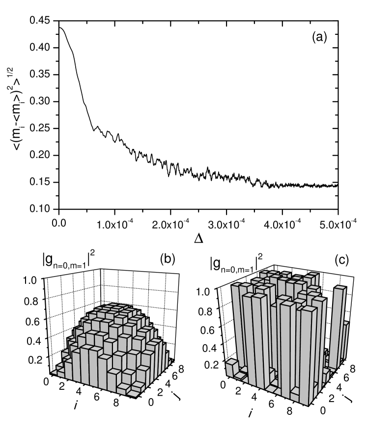
Figure 9: Dynamical crossover from the Fermi gas to the Fermi glass phases. The parameters are the same as in Fig. 8(c). (a) Variance of the number of fermions per lattice site as a function of the amplitude of the disorder $\Delta$. (b) Probability of having one composite (one fermion and zero boson) at each lattice site for the M sites in the absence of disorder and (c) after ramping up adiabatically diagonal disorder with amplitude $\Delta=5\times 10^{-4}$.

We now consider the Fermi insulator domain phase (see Fig. 10(b)) with slowly increasing disorder. In the Fermi insulator domain (in the absence of disorder), the composite fermions are pinned in the central part of the confining potential. In addition, there is a ring of delocalized fermions and this gives finite fluctuations on the atom number per site ($\sqrt{\langle(m_{i}-\langle m_{i}\rangle)^{2}\rangle}\simeq 0.35$). As shown in Fig. 10(a), while ramping up the amplitude of disorder, the fluctuations decrease fast and reach ($\sqrt{\langle(m_{i}-\langle m_{i}\rangle)^{2}\rangle}\simeq 0.13$ for $\Delta>10^{-4}$. This indicates that the composite fermions are pinned in different lattice sites. This is confirmed in Fig. 10(c) where we plot the population of the composites fermions in each lattice site for $\Delta=5\times 10^{-4}$. Contrary to what happens for the transition from Fermi gas to Fermi glass, the composites mostly populate the central part of the confining potential. The reason for that is twofold. First, with our parameters, the attractive interaction between composites is of the order of $K\simeq-1.4\times 10^{-3}$ and can compete with disorder $\Delta=3\times 10^{-4}$. This explains the central insulator domain. Second, because tunneling is small ($d\simeq 8\times 10^{-5}$) and because disorder breaks the symmetry of lattice sites in the ring around the domain, the atoms in this region get pinned. The populated sites match the lowest $\tilde{\mu}_{i}^{\textrm{b}}$.

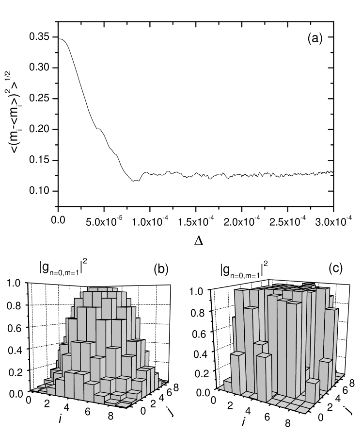
Figure 10: Dynamical crossover from the fermionic domain insulator to a disordered insulating phase. The parameters correspond to Fig. 8(d). (a) Variance of the number of fermions per lattice site as a function of the amplitude of the disorder. (b) Probability of having one composite (one fermion and zero boson) in each lattice site in the absence of disorder and (c) after ramping up adiabatically the disorder with amplitude $\Delta=3\times 10^{-4}$.

V Spin glasses

In this chapter we discuss in more detail the possible realization of the Edwards-Anderson spin glass Fermi-Bose mixtures as discussed in section III.3. Strictly speaking, since the system is quantum it allows for realization of fermionic spin glass oppermann . The main goal of such investigation is to study the nature of the spin glass ordering and to compare the predictions of the Mézard-Parisi and ”droplet” pictures.

Although we work along the lines of the original papers parisi , it is necessary to reformulate the standard Mézard-Parisi mean field description of our system. The main difference appears because the Ising spins are coded as presence or absence of a composite at a given site. This leads to a fixed magnetization due to the fixed number of particles in the system. For this we repeat very shortly the Sherrington-Kirkpatrick calculations sherr here, adapted to our case.

V.1 Edwards-Anderson model for composite fermions

The spin glass limit obtained in section III.3 with large disorder derives of the composite fermionic model (7) with vanishing hopping due to strong site-to-site energy fluctuations and n.n.-interactions, $K_{ij}$. By appropriate choice of $\Delta_{ij}^{\textrm{b}}$, $K_{ij}$ fluctuate around mean zero with random positive and negative values (see Fig. 2(b)). Replacing the composite number operators with a classical Ising spin variable $s_{i}:=2M_{i}-1=\pm 1$, one ends up with the Hamiltonian:

$$H_{\textrm{E-A}}=\frac{1}{4}\sum_{\left\langle ij\right\rangle}K_{ij}s_{i}s_{j}+\frac{1}{2}\sum_{i}\overline{\mu}_{i}s_{i},$$ (26)

It describes an (fermionic) Ising spin glass oppermann , which differs from the Edwards-Anderson model binder ; parisi in that it has an additional random magnetic field $\overline{\mu}_{i}$ and moreover has to satisfy the constraint of fixed magnetization value, $m=2N_{\textrm{f}}/N-1$, as the number of fermions in the underlying BFH-model is conserved. It however shares the basic characteristics with the Edwards-Anderson model as being a spin Hamiltonian with random spin exchange terms $K_{ij}$. In particular, this provides bond frustration, which in this model is essential for the appearance of a spin glassy phase. The experimental study of this limit thus could present a way to address various open questions of spin glass physics concerning the nature and the ordering of its ground- and possibly metastable states (the Mézard-Parisi picture parisi versus the “droplet” picture huse ; stein ), broken symmetry and dynamics in classical (in absence of hopping) and quantum (with small, but nevertheless present hopping) spin glasses sachdev ; georges .

For sufficiently large systems, Eq. (26) is well approximated by assuming $K_{ij}$ and $\overline{\mu}_{i}$ to be independent random variables with Gaussian distribution, with mean $0$ and $H$, respectively and variances $K/\sqrt{N}$ and $h$, respectively foot5 . This approximation will be used in the following calculations.

Before employing the mean field approach for Edwards-Anderson-like models in section V.5 for the Hamiltonian (26), a very basic outline of the different phases of the short-range Ising models with bond frustration is given and the two competing physical pictures for the spin glass phase are briefly summarized in this section.

The experimental observations have led to the identification of three equilibrium phases, which are characterized by two order parameters (for zero external magnetic field): $M:=\overline{\left\langle s_{i}\right\rangle_{T}}$ is the magnetization, i.e., the order parameter for magnetic ordering, and $Q_{EA}:=\overline{\left\langle s_{i}\right\rangle_{T}^{2}}$ is the Edwards-Anderson order parameter for spin glass ordering. Here, $\left\langle\cdot\right\rangle_{T}$ denotes the Gibbs ensemble average and $\overline{\hskip 2.84544pt\cdot\hskip 2.84544pt}$ the disorder average. The three phases are: (i) an unordered paramagnetic phase, with $M=0$ and $Q_{EA}=0$; (ii) an ordered spin glass phase with $M=0$ and $Q_{EA}\neq 0$ that is separated from the paramagnetic phase by a second order phase transition foot6 ; and (iii) dependent on the mean value of $K_{ij}$, an ordered ferromagnetic phase with $M\neq 0$ and $Q_{EA}=0$. It should be pointed out that there are additional questions - different from, but of course connected to the ones discussed in the following - about the nature of the equilibrium spin glass state that stem from the intrinsic problems that are associated in this system with separating equilibrium from non equilibrium effects such as metastability, hysteresis and others (see refrigier and references therein).

V.2 Mézard-Parisi picture

The Mézard-Parisi (MP) picture is fundamentally guided by the results of the mean-field theory. On the level of statistical physics, the Gibbs equilibrium distribution of the spin system in the MP-picture at temperature $T$ and for a particular disorder configuration $K$ can be written as a unique convex combination of infinitely many pure equilibrium state distributions vanenter ; stein ,

$$\rho_{T,K}=\sum_{\alpha}w^{\alpha}_{T,K}\rho^{\alpha}_{T,K},\quad\mbox{with}\quad\sum_{\alpha}w^{\alpha}_{T,K}=1$$ (27)

where the overlap between two pure states is defined as

$$Q_{\alpha\beta}\equiv\Omega^{-1}\sum_{i}\left\langle s_{i}\right\rangle_{T,K}^{\alpha}\left\langle s_{i}\right\rangle_{T,K}^{\beta}$$ (28)

where $\Omega$ denotes the size of the system. The mean-field version of $Q_{\alpha\beta}$ emerges naturally from the calculation in the next section and motivates definition (28).

In the MP-picture, the spin glass transition is interpreted akin to the transition from an Ising paramagnet to a ferromagnet. There, the Gibbs distribution is written as a sum of only two pure states, corresponding to the two possible fully spin-polarised ferromagnetic ground states. As the temperature of the system decreases, the $Z_{2}$ symmetry of the system is broken, and a phase transition to a ferromagnetic phase occurs, whose equilibrium properties are not described by the Gibbs state, but by the relevant pure state distribution alone parisi . Analogously, the spin glass transition is characterized by the breaking of the infinite index symmetry, called replica symmetry breaking in the mean-field case, by which one pure state distribution $\rho^{\alpha}_{T,K}$ is chosen and alone describes the low-temperature properties of the system parisi . However, unlike the Ising ferromagnet, the pure states of the spin glass are not related to each other by a symmetry of the Hamiltonian, but rather by an accidental, infinite degeneracy of the ground state caused by the randomness of the bonds and the frustration effects. This picture can be interpreted as the system getting frozen into one particular state out of infinitely many different ground- or metastable states of the system. These states are all taken to be separated by free energy barriers, whose height either diverges with the system size or it is finite but still so large that the decay into a ”true” ground state does not occur on observable timescales. Thus, fluctuations around one of these ground states can only sample excited states within one particular free energy valley. Consequently, $Q_{EA}$ in the spin glass phase must be redefined as $Q_{EA}:=Q_{\alpha\alpha}$, the self-overlap of the state, whereas it remains unchanged for the paramagnetic phase.

V.3 de Almeida-Thouless plane

Based on the results of mean-field theory, one of the predictions of the MP-picture concerns the order of the infinitely many spin glass ground states, which is ultrametric parisi ; foot7 , as can be seen from the joint probability distribution of three different ground state overlaps, $P_{K}(Q_{12},Q_{13},Q_{23})$. Upon choosing independently three pure states $1$, $2$ and $3$ from the decomposition (27), one should find that with probability $1/4$, $Q_{12}=Q_{13}=Q_{23}$ and with probability $3/4$ two of the overlaps are equal and smaller than the third. Ultrametricity then follows from the canonical distance function $D_{\alpha\beta}=Q_{EA}-Q_{\alpha\beta}$. The mean-field theory, both with and without a magnetic field, predicts the existence of a plane in the space of the Hamiltonian parameters, called de Almeida-Thouless (dAT) plane at , below which the naive ansatz for the spin glass phase becomes invalid and the system is characterized by the transition to this ultrametrically ordered infinite manifold of ground states. It should be pointed out that the clear occurrence of such a dAT-plane in the finite range Edwards-Anderson model would be an important indicator for the validity of the MP-picture in these systems. As we discuss in section V.4, this conclusion has to be drawn with great care.

V.4 ”Droplet” model

The very applicability of the MP-model for finite-range systems is however still unproven. It is both challenged by a rival theory, the so-called droplet model huse , as well as by mathematical analysis (cf. stein and references therein) that questions the validity of transferring a picture developed for the infinite-range mean-field case to the short-range model. Being a phenomenological theory based on scaling arguments and numerical results, the droplet model describes the ordered spin glass phase below the transition as one of just two possible pure states, connected by spin-flip symmetry, analogous to the ferromagnet mentioned above. Consequently there can be no infinite hierarchy of any kind, and thereby no ultrametricity. Excitations over the ground state are regions with a fractal boundary - the droplets - in which the spins are in the configuration of the opposite ground-state. The free energy of droplets of diameter $L$ is taken to scale as $\sim L^{\theta}$, with $\theta<0$ at and below the critical dimension, which is generally taken to be two. So three is the only physical dimension where the spin glass transition is stable with nonzero transition temperature, with $\theta\sim 0.2$ in this case. The free energy barriers for the creation and annihilation of a droplet scales in 3D as $\sim L^{\psi}$, with $\theta\leq\psi\leq 2$.

Although there can be no dAT-plane in the strict sense in the droplet-model, for an external magnetic field the system can be kept from equilibration on experimental timescales for parameters below a line that scales just like the dAT-line. This phenomenon might mimic the effects of the replica symmetry-breaking in the MP-picture (see huse for further details).

V.5 Replica-symmetric solution for fixed magnetization

This section serves to show that the mean-field version of the effective Hamiltonian (26) with random magnetic field and magnetization constraint exhibits replica symmetry breaking just as for the pure Edwards-Anderson model, and would therefore be a candidate to examine the validity of the MP or droplet-picture in a realistic short-ranged spin-glass model. Following Sherrington and Kirkpatrick (SK) parisi , the mean-field model is given by:

$$H_{SK}=\frac{1}{4}\sum_{(i,j)}K_{ij}s_{i}s_{j}+\frac{1}{2}\sum_{i}\overline{\mu}_{i}s_{i}$$ (29)

where the round brackets $(\cdot,\cdot)$ are generally used to denote sums over all pairs of different indices. This model differs from Eq. (26) by the long-range spin exchange. As the mean of $\overline{\mu}_{i}$, $H$, is generally nonzero this model will not exhibit a phase transition, which however is not a concern, as the number of (quasi-)ground states will be the quantity of interest. Following the analysis of SK, we aim at finding the free energy, ground state overlap and magnetization constraint. Then we will use the de Almeida and Thouless approach parisi to show that the obtained solution is unstable in a certain parameter region, that lies below the so-called dAT-plane of stability. The type of instability that emerges is then well known to require the replica symmetry breaking solution of Parisi parisi .

As the disorder is quenched (static on experimental timescales), one cannot average directly over disorder in the partition function as would be done for annealed disorder, but one must rather average the free energy density, $\overline{f}=-\beta\overline{\ln Z}$ using the ’replica trick’: We form $n$ identical copies of the system (the replicas) and the average is calculated for an integer $n$ and a finite number of spins $N$. Then, using the general formula $\ln x=\lim_{n\rightarrow 0}(x^{n}-1)/n$, $\overline{\ln Z}$ is obtained from the analytic continuation of $\overline{Z^{n}}$ for $n\rightarrow 0$. Finally, we take the thermodynamic limit $N\rightarrow\infty$. Explicitly, $\overline{Z^{n}}$ is given by:

$$\overline{Z^{n}}=\sum_{\{s_{i}^{\alpha}=\pm 1\}}\exp\left[-\beta\overline{H[s_{i}^{\alpha},n]}\right]$$ (30)

where $\overline{H_{SK}[s_{i}^{\alpha},n]}$ is the sum of $n$ independent and indentical spin Hamiltonians (29), averaged over the Gaussian disorder, with Greek indices now numbering the $n$ replicas.

Executing the average over the Gaussian distributions for $K_{ij}$ and $\overline{\mu}_{i}$ leads to coupling between spin-spin-interactions of different replicas. As the mean-field approach means that the double sum over the site indices in (29) can be simplified into a square using $(s_{i}^{\alpha})^{2}=1$, one finds:

$$\overline{f_{N}^{n}}=-(Nn\beta)^{-1}\left\{e^{Nn(\beta K)^{2}/4}e^{-n^{2}(\beta K)^{2}/2+n(\beta h)^{2}/2}\sum_{\left\{s_{i}^{\alpha}=\pm 1\right\}}\exp\left[\frac{N(\beta K)^{2}}{2}\sum_{\alpha<\beta}\left(\sum_{i}\frac{s_{i}^{\alpha}s_{i}^{\beta}}{N}\right)^{2}\right.\right.$$ (31)

$$\left.\left.+(\beta h)^{2}\sum_{\alpha<\beta}\sum_{i}s_{i}^{\alpha}s_{i}^{\beta}-\beta H\sum_{\alpha}\sum_{i}s_{i}^{\alpha}\right]-1\right\}$$

where the prefactor $e^{-n^{2}(\beta K)^{2}/2+n(\beta h)^{2}n/2}$ becomes irrelevant in the limit $n\rightarrow 0$ and is subsequently dropped. As in the standard procedure, the square of the operator sum $\sum_{i}$$s_{i}^{\alpha}$$s_{i}^{\beta}$ is decoupled by introducing auxiliary operators $q_{\alpha\beta}$ via a Hubbard-Stratonovitch transformation parisi .

$$\overline{f_{N}^{n}}=-(Nn\beta)^{-1}\left\{e^{Nn(\beta K)^{2}/4}\int_{-\infty}^{\infty}\left[\prod_{\alpha<\beta}dq_{\alpha\beta}\left(\frac{N}{2\pi}\right)^{\frac{1}{2}}\beta K\right]\right.$$ (32)

$$\left.\times\exp\left[-\frac{N(\beta K)^{2}}{2}\sum_{\alpha<\beta}q_{\alpha\beta}^{2}+N\ln\left(\sum_{\left\{s^{\alpha}=\pm 1\right\}}\exp\left[L(q_{\alpha\beta})\right]\right)\right]-1\right\}$$

where the functional $L(q_{\alpha\beta})$ is:

$$L(q_{\alpha\beta})=\beta^{2}\sum_{\alpha<\beta}\left(K^{2}q_{\alpha\beta}+h^{2}\right)s^{\alpha}s^{\beta}-\beta H\sum_{\alpha}s^{\alpha}$$ (33)

and the configuration sum of $\exp\left[L(q_{\alpha\beta})\right]$ now only goes over the $n$ spins $s^{\alpha}$ in $L(q_{\alpha\beta})$, the HS-transformation having made it possible to decouple the configuration sum over $Nn$ spins in (31) into a $N$-fold product of $n$-spin sums. Assuming that the thermodynamic limit ($N\rightarrow\infty$) can be taken before $n\rightarrow 0$, i.e., that the usual limiting process can be inverted, then Eq. (32) can be evaluated by the method of steepest descent, as the exponent is proportional to $N$. According to this method, the free energy per spin in the thermodynamic limit is the maximum of the $q_{\alpha\beta}$-dependent function in the exponent:

$$-\beta\overline{f}=\lim_{n\rightarrow 0}\max\left\{\frac{(\beta K)^{2}}{4}\left(1-\frac{1}{n}\sum_{(\alpha,\beta)}q_{\alpha\beta}^{2}\right)+\frac{1}{n}\ln\left(\sum_{\left\{s^{\alpha}=\pm 1\right\}}\exp\left[L(q_{\alpha\beta})\right]\right)\right\}$$ (34)

(with $\overline{f}:=\lim_{n\rightarrow 0}\overline{f^{n}}$) with the self-consistency condition:

$$\frac{\partial\overline{f}}{\partial q_{\alpha\beta}}=0\quad\Leftrightarrow\quad q_{\alpha\beta}=\langle s^{\alpha}s^{\beta}\rangle_{L}$$ (35)

and the magnetization:

$$m=-\frac{1}{\beta}\frac{\partial\overline{f}}{\partial H}=\langle s^{\alpha}\rangle_{L}=2N_{F}/N-1$$ (36)

where the average $\langle(\cdot)\rangle_{L}$ is defined as:

$$\langle(\cdot)\rangle_{L}=\lim_{n\rightarrow 0}\frac{\sum_{\left\{s^{\alpha}=\pm 1\right\}}(\cdot)\exp\left[L(q_{\alpha\beta})\right]}{\sum_{\left\{s^{\alpha}=\pm 1\right\}}\exp\left[L(q_{\alpha\beta})\right]}$$ (37)

The mean-field approach has allowed a decoupling of the spins, and a reduction of the problem to a single-site model with ”Hamiltonian” $L[q_{\alpha\beta}]$. For this new problem, the overlap parameter emerges naturally, albeit in a self-consistent manner. To push the calculation further some assumption for $q_{\alpha\beta}$ has to be made. Naively, from the requirement that the result should be independent of the replica-indices, the most natural choice for $q$ is to consider all identical overlaps between the replicas, $q_{\alpha\beta}=q$, which is the SK-ansatz. Thus the double sum over the replicas $\sum_{(\alpha,\beta)}s^{\alpha}s^{\beta}$ in (33) can be written as a square, keeping $(s^{\alpha})^{2}=1$ in mind. Another Hubbard-Stratonovitch-transformation with auxiliary variable $z$ then decouples the square and yields an expression for the free energy density, which has to be evaluated self-consistently and in which the limit $n\rightarrow 0$ can be easily calculated:

$$-\beta\overline{f}_{SK}=\lim_{n\rightarrow 0}\left\{\frac{(\beta K)^{2}}{4}\left(1-(n-1)q^{2}\right)+\frac{1}{n}\ln\left(\frac{1}{\sqrt{2\pi}}\int_{-\infty}^{\infty}dz\exp\left[-\frac{z^{2}}{2}\right]\right.\right.$$ (38)

$$\left.\left.\times\left(\exp\left[-\frac{\beta^{2}(K^{2}q+h^{2})}{2}\right]\sum_{s=\pm 1}\exp\left[\beta\sqrt{K^{2}q+h^{2}}s-\beta Hs\right]\right)^{n}\right)\right\}$$

$$\Rightarrow\beta\overline{f}_{SK}=\frac{(\beta K)^{2}}{4}\left(1-q\right)^{2}-\frac{(\beta h)^{2}}{2}+\left(\frac{1}{2\pi}\right)^{\frac{1}{2}}\int_{-\infty}^{\infty}dze^{-\frac{z^{2}}{2}}\ln\left(2\cosh(A(z))\right)$$ (39)

with $A(z):=\beta\sqrt{K^{2}q+h^{2}}-\beta H$. The overlap (35) and the magnetization constraint (36) can also be evaluated in the same way:

$$q=\frac{1}{\sqrt{2\pi}}\int_{-\infty}^{\infty}dze^{-\frac{z^{2}}{2}}\tanh^{2}(A(z))$$ (40)

$$m=\frac{1}{\sqrt{2\pi}}\int_{-\infty}^{\infty}dze^{-\frac{z^{2}}{2}}\tanh(A(z))=2N_{F}/N-1~{}.$$ (41)

A well known problem with the SK-ansatz for $q_{\alpha\beta}$ is that it yields negative entropy for low temperatures and thus becomes unphysical. This is due to a fundamental technical problem with the replica trick: For the method of steepest descent to be valid, the SK-solution must be a maximum of the exponent in Eq. (32) and must stay a maximum as the replica-limit $n\rightarrow 0$ is taken. But there is no unique way of choosing the zero-dimensional limit of the matrix $q_{\alpha\beta}$. The SK-solution just corresponds to one possible choice for this limit. Thus, the question arises whether the SK-solution for the free energy is still a good, i.e., maximal choice in the replica limit.

To answer this question, one proceeds analogous to the de Almeida and Thouless procedure at to analyze the fluctuations around the SK-solution, while taking the magnetization constraint into account (see appendix B for details). Developing (34) and (36) to second and first order respectively around $q_{\alpha\beta}=q$ one finds that in the replica limit $n\rightarrow 0$ there is an eigenvalue $\lambda_{2}$ of the matrix $\partial^{2}\overline{f}/\partial q_{\alpha\beta}\partial q_{\gamma\delta}$ that can have both negative values and respects the constraint, yielding the condition:

$$\lambda_{2}=\frac{1}{(\beta K)^{2}}-\frac{1}{\sqrt{2\pi}}\int_{-\infty}^{\infty}dze^{-\frac{z^{2}}{2}}\mbox{sech}^{4}(A(z))>0$$ (42)

which is violated for low enough $T/K$, $H/K$ and $h/K$. The plane in parameter space below which this happens is the so-called dAT-surface. This instability is rectified by a much more involved ansatz for $q_{\alpha\beta}$ that breaks the symmetry of the replicas and leads to the phenomena described in section A.

VI Experimental insights

Experimental creation and detection of the phenomena discussed in this paper poses a major problem, and deserves itself a lot of creative thinking and separate publications. In this section we will just sketch, what are in our opinion the most obvious ways of addressing these problems. In this section we do not address the questions concerning experimental realization of ultracold FB mixtures and composite fermions - these questions are discussed in Ref. fb .

The first question thus to be addressed is what are the best ways to create quenched disorder in a controlled way. Roth and Burnett keith and we boseglass have suggested that the use of pseudo-random disorder induced by non-commensurate optical lattices should work as well as the use of the genuine random lattices. Indeed the latter can be only (so far) achieved using speckle radiation, i.e. disorder correlation length of order of few microns! If we work with systems of size of mm’s, such disorder would definitely be enough to induce localization in 1D, or 2D. Unfortunately, the size of the systems in question is typically is of order of hundred microns, and that is one of the reasons, why it is difficult to observe Anderson localization with BEC’s inguscio ; aspect .

The analysis performed by us in this context implies clearly that it will be much easier to achieve the desired properties of the disorder using pseudo-disordered, i.e., overlapped incommensurable optical lattices arlt . One should also stress the equally promising look to the proposals formulated recently to use the optical tweezers techniques privat3 and a random distribution of impurity atoms pinned in different lattice sites privat1 .

Completely another variety of problems is related to the detection of the quantum phases discussed in this paper. Below we list basic mehtods that have been already successfully applied to ultracold atomic gases in optical lattices.

• Imaging of the atomic cloud after ballistic expansion. This (perhaps the most standard method) has been used in Ref. bloch to distinguish the bosonic SF phase from the MI phase. It allows for measurement of the quasi-momentum distribution of atoms obtained after initial expansion caused by interactions fermisur , i.e., it detects first order coherence (interference pattern), present for instance in the SF phase.

• Monitoring the density profile.Using phase contrast imaging ketterlehulet it is possible to perform a direct and non-destructive observation of the spatial distribution of the condensate in situ. This kind of measurement allows the direct observation of superfluidity ketterlem2 and can be therefore applied to characterize the fluid and superfluid phases.

• Tilting or acceleration of the lattice. This method was used in Ref. blochnat2 to detect the gap in the MI phase. It allows, in principle, to distinguish gapless from gapped phases, provided the continuum of low energy states can be achieved via tilting. Fluidity, superfluidity, and in general extended, non-localized excitations should allow to detect Bloch oscillations blochosc .

• Absorption of energy via modulation of the lattice. This method was also designed to detect the gap in the MI phase esslinger . Similarly as tilting, it provides a way of probing excitations in the systems.

• Bragg spectroscopy. This method, one of the first proposed stenger , is also a way of probing certain kind of excitations in the system orsayelongated .

• Cooper pair spectroscopy. This method is particularly useful to detect Fermi superfluids revBCS . Its theoretical aspects are discussed in Refs. paivi , while for experiments see Ref. grimm .

• Trap shaking and nonlinear dynamics. Yet another way to probe excitations could correspond to analysis of the response of the system upon sudden shaking of the trap lukin .

• Observations of vortices, solitons etc. This method provides a direct way to detect superfluidity (for vortices in Bose superfluid see for instance Ref. jean , for vortices in Fermi superfluid see ketterlelast ).

• Spatial quantum noise interferometry. The last, but not the least method discussed here allows for practically direct measurement of the density-density correlation, and second order coherence. It has been proposed in Ref. altman (see also kazik ), and used with great success to detect the bosonic Mott insulator follig and the Fermi superfluid greinernat . It has capabilities of detecting and measuring relevant properties of various phases and structures ranging from supersolids, charge-density wave phases, and even Luttinger liquids in 1D. In the Fourier frequency and momentum domain it corresponds to measurements of the dynamic structure factor (for a discussion in the context of cold gases see Ref. rothstruc .

There are of course more methods than the ones discussed above, but combined applications of those discussed should allow for clear detection and characterization of the quantum phases discussed in this paper.

Let us start this discussion with ideal Fermi gas, Fermi liquid and metaling phases between Fermi glass and glassy Mott insulator. All of them are fluids, i.e. will respond consequently to perturbations. They are gappless, and differ in this sense from the Fermi superfluids. All of them should lead to a nontrivial Fermi surface imaging in ballistic expansion. Difference between ideal, and interacting phases is here rather quantitative, and as such can be measured. Quantities such as the effective mass can be recovered from the measurements. Influence of disorded on these phase will be seen as gradual decrase of their ”conducting” properties. Similar scenario is expected to take place with ”dirty” superfluids; here measurements of the gap (using any of the excitation probing methods) should reveal rapid gap decrease with the increasing disorder.

Disordered and glassy phases, such as Femi glass of glassy Mott insulator are more difficult to detect. Obviously they will tend to give blurred images in the measurement of the first order coherence. Spatial noise interferometry should reveal some information about the glassy Mott insulator, especially in the region of parameters where it will incorporate domains of checker board phase. Although the glassy phases are gapless, the states forming the spectral quasi-continuum at low energies may be very difficult to achieve in simple excitation measurements, since they may lie far away one from another in the phase space. Probing of one of such states would thus allow to study excitations accesible locally in the phase, which most presumably will be gapped. The character of excitations, and in particular their spectrum should, however, be a very sensitive function of how one excites them, and how one detects them (compare lukin ). On the other hand, domain insulator phase should be visible by ”naked eye”, and independent detection of bosons and composites. Also, the noise interferometry should reveal informations about the presence of the lattice, similarly as in the standard Mott insulator phase follig .

Finally, a separate problem concerns detection of the fermionic spin glass phase and its properties, as well as distinction between the possible adequacy of Parisi versus droplet model. Repeated preparation of the system in the lattice with the same disorder (or even direct comparison and measurement of overlap of replicas zollerhp ) will shed some light on the latter problem. In many other aspects, response of the spin glass to excitations will be similar to that of Fermi glasses and glassy Mott insulator.

VII Conclusions

Summarizing, we have studied atomic Fermi-Bose mixtures in optical lattices in the strong interacting limit, and in the presence of an inhomogeneous, or random on-site potential. We have derived the effective Hamiltonian describing the low temperature physics of the system, and shown that an inhomogeneous potential may be efficiently used to control the nature and strength of (boson mediated) interactions in the system. Using a random potential, one is able to control the system in such a way that its physics corresponds to a wide variety of quantum disordered systems. It is worth mentioning that the physics discussed in this paper is very much analogous to the one of Bose-Bose mixtures in the limit of hard core bosons (when both species exhibit strong intraspecies repulsion).

We end this section with a general comment on quantum complex systems. In our opinion quantum degenerate gases offer an absolutely unique possibility to study various models of physics of disorder systems, such as Bose and Fermi glasses, quantum percolating systems, ”dirty” superfluids, domain and Mott insulators, quantum spin glasses, systems exhibiting localization-delocalization phenomena, etc. The summary of predictions of this paper is schematically shown in the following list of quantum phases, obtained for the case of only one type of sites, and $\mu_{i}^{\textrm{f}}=0$, or $\mu_{i}^{\textrm{f}}=\mu_{i}^{\textrm{b}}$:

• Composites $I$ - Fermi liquid, Fermi glass, quantum bond percolation;

• Composites $II$ - ideal Fermi gas, Fermi glass, Fermi liquid, Mott Insulator, fermionic spin glass;

• Composites $\overline{II}$ - domain insulator, ”dirty” superfluid, Fermi glass, metallic phase, Mott insulator, fermionic spin glass.

Additionally, for the case of lattices with different types of sites, physics of quantum site percolation will become relevant. Complex systems such as quantum celular automata, or neural networks can also be realized in this way. In fact, we and other authors have several times already stressed the fascinating possibility of using the ultracold lattice gases as quantum simulators of complex systems. But, the proposed systems go beyond just repeating what is known from the other kinds of physics; they allow to create novel quantum phases and novel quantum behaviors.

We thank M. Baranov, H.-P. Büchler, B. Damski, M. Dressel, A. Georges, A. Niederberger, J. Parrondo, L. Santos, A. Sen (De), U. Sen, G.V. Shlyapnikov, J. Wehr and P. Zoller for fruitful discussions. We acknowledge support from the Deutsche Forschungsgemeinschaft (SFB 407, SPP1116 436POL), the RTN Cold Quantum Gases, ESF PESC QUDEDIS, the Alexander von Humboldt Foundation and Ministerio de Ciencia y Tecnologia (BFM-2002-02588). V.A. acknowledges support from the European Community (MEIF-CT-2003 -501075).

Appendix A Effective Hamiltonian to Second Order

The Hamiltonian of our 2-species system described in III.2 splits into two components: $H_{0}$ and $H_{int}$. The Hamiltonian $H_{0}$ has known eigenstates, that are grouped in blocks (or manifolds) of states close in energy while the differences between states from two different blocks are much larger than the intrablock spacing. In the case of section III.2, this corresponds to the manifold of near-ground states, separated in energy by terms of order $\Delta_{ij}^{\textrm{b,f}}$, which is separated from other blocks of higher excited states (two or more bosons in one site) by terms of the order $V$. Generally, the projector on each block space is denoted by $P_{\alpha}$  where $\alpha$ is the block index, and the $i$-th state in any block is denoted by $|\alpha,i\rangle$. Note that $P_{\alpha}H_{0}P_{\beta}=0$ holds for $\alpha\neq\beta$.

The second component is a Hamiltonian, $H_{int}$, that couples to $H_{0}$ via a factor $J$, where $J$ is considered to be small, to form the complete Hamiltonian of the system, $H=H_{0}+JH_{int}$. The interaction Hamiltonian is now considered to introduce couplings between block $\alpha$ and $\beta$, i.e., $P_{\alpha}H_{int}P_{\beta}\neq 0$ for $\alpha\neq\beta$.

Following the technique detailed e.g. in cohen , we construct an effective Hamiltonian, $H_{eff}$  from $H$ such that it describes the slow, low-energy perturbation-induced tunneling strictly within each manifold of unperturbed block states, i.e., $P_{\alpha}H_{eff}P_{\beta}=0$ for $\alpha\neq\beta$, and has the same eigenvalues as $H$. Tunneling between different blocks is thus neglected, as this corresponds to fast, high-frequency processes which we neglect here. Technically, the requirements for $H_{eff}$ are:

1. $H_{eff}$ is hermitian, with the same eigenvalues and the same degeneracies as $H$. To achieve this, one defines $T:=e^{iS}$, with $S$ hermitian, $S=S^{\dagger}$, and chosen such that:

   $$H_{eff}=THT^{\dagger}~{}.$$ (43)

2. $H_{eff}$ does not couple states from different manifolds:

   $$P_{\alpha}H_{eff}P_{\beta}=0,\quad\alpha\neq\beta\quad~{}.$$ (44)

3. As the first two conditions still allow for an infinite number of unitary transformations (all $UT$ are still possible, $U$ being any unitary transformation acting only within the manifolds), the following additional condition is imposed:

   $$P_{\alpha}SP_{\alpha}=0\quad\mbox{for any}\hskip 2.84544pt\alpha$$ (45)

Expanding the first condition using the Baker-Hausdorff formula, one obtains:

$$H_{eff}=H+\left[iS,H\right]+\frac{1}{2!}\left[iS,\left[iS,H\right]\right]$$ (46)

$$+\frac{1}{3!}\left[iS,\left[iS,\left[iS,H\right]\right]\right]+\ldots$$

Making a power-series ansatz in $S$,

$$S=JS_{1}+J^{2}S_{2}+J^{3}S_{3}+\ldots,$$ (47)

and employing $H=H_{0}+JH_{int}$ one obtains from (46) to second order

$$H_{eff}=H_{0}+J\overbrace{\left(\left[iS_{1},H_{0}\right]+H_{int}\right)}^{H_{eff}^{1}}\hskip 28.45274pt$$

$$+J^{2}\overbrace{\left(\left[iS_{2},H_{0}\right]+\left[iS_{1},H_{int}\right]+\frac{1}{2}\left[iS_{1},\left[iS_{1},H_{0}\right]\right]\right)}^{H_{eff}^{2}}~{}.$$ (48)

This is a power series for $H_{eff}$, with its moments denoted by $H_{eff}^{1}$, $H_{eff}^{2}$, $\ldots$ , where $H_{eff}^{n}$ generally depends on all $S_{j}$ with $1\leq j\leq n$. This allows for a systematic evaluation of the matrix elements $\langle\alpha,i|iS_{j}|\beta,j\rangle$, and consequently delivers matrix expressions for the $H_{eff}^{j}$ and $H_{eff}$.

To start with this, one considers the expansions (48) and (47) up to first order, i.e. $H_{eff}=H_{0}+JH_{eff}^{1}$ and $S=JS_{1}$. Using the second and third conditions, as well as $P_{\alpha}H_{0}P_{\beta}=0$ and the expression for $H_{eff}^{1}$ in (48), one finds:

$$\langle\alpha,i|iS_{1}|\beta,j\rangle\left(E_{\beta j}-E_{\alpha i}\right)+\langle\alpha,i|H_{int}|\beta,j\rangle=0$$ (49)

$$\Rightarrow\langle\alpha,i|iS_{1}|\beta,j\rangle=\left\{\begin{array}[]{cr}\frac{\langle\alpha,i|H_{int}|\beta,j\rangle}{E_{\alpha i}-E_{\beta j}}&\alpha\neq\beta\\ 0&\alpha=\beta\end{array}\right.~{}.$$ (50)

Thus, the effective Hamiltonian within the $\alpha$-manifold, depends only on the interaction term and not on $S_{1}$, i.e., $\langle\alpha,i|H_{eff}^{1}|\alpha,j\rangle=\langle\alpha,i|H_{int}|\alpha,j\rangle$. A general result for any $n$ is that $\langle\alpha,i|H_{eff}^{n}|\alpha,j\rangle$ is independent of $S_{n}$. Based on the third condition, and on the observation that $S_{n}$ enters the expression for $H_{eff}^{n}$ only in the commutator with $H_{0}$, which is diagonal in the manifold index.

Thus, when continuing to second order, the term $\left[iS_{2},H_{0}\right]$ in the expression for $H_{eff}^{2}$ can be dropped. Of the two remaining terms defining $H_{eff}^{2}$ in (48), the second one can be simplified by observing, that according to (49) the operator $[iS_{1},H_{0}]$ is purely non-diagonal in the manifold index, with values opposite to those of the non-diagonal part of the interaction Hamiltonian. Thus, $\frac{1}{2}\left[iS_{1},\left[iS_{1},H_{0}\right]\right]=-\frac{1}{2}\left[iS_{1},H_{int}^{nd}\right]$. Now inserting the identity between the operators in the still untreated second term in $H_{eff}^{2}$, $\left[iS_{1},H_{int}\right]$ , one sees that due to $S_{1}$ being non-diagonal in $\alpha$, again only the non-diagonal part of $H_{int}$ can contribute: $\left[iS_{1},H_{int}\right]=\left[iS_{1},H_{int}^{nd}\right]$. Therefore, one has:

$$H_{eff}^{2}=[iS_{1},H_{int}^{nd}]+\frac{1}{2}[iS_{1},\overbrace{\left[iS_{1},H_{0}\right]}^{-H_{int}^{nd}}]=\frac{1}{2}[iS_{1},H_{int}^{nd}]~{}.$$ (51)

Collecting all terms relevant for $\langle\alpha,i|$$H_{eff}$$|\alpha,j\rangle$ to second order in $J$, and introducing the notation $Q_{\alpha i}:=\sum_{k,\gamma\neq\alpha}\frac{|\gamma,k\rangle\langle\gamma,k|}{E_{\gamma k}-E_{\alpha i}}$, one finds:

$$\langle\alpha,i|H_{eff}|\alpha,j\rangle=E_{\alpha i}\delta_{ij}+J\langle\alpha,i|H_{int}|\alpha,j\rangle$$

$$-\frac{J^{2}}{2}\left(\langle\alpha,i|H_{int}\left[Q_{\alpha i}+Q_{\alpha j}\right]H_{int}|\alpha,j\rangle\right)$$ (52)

where the identity operator has been inserted in the final expression for $H_{eff}^{2}$ in formula (51), and then evaluated using formula (50), which naturally leads one to define the operator $Q_{\alpha i}$ as above. Note that this construction can be generalized to arbitrary orders in $J$ in a straightforward manner, as detailed in cohen .

Appendix B Stability of the SK-solution

The Taylor-expansion of Eq. (34) around $q_{\alpha\beta}=q$ yields the correction $-\frac{1}{2}\delta\overline{f}$ to the free energy, with:

$$\delta\overline{f}=\sum_{\left[\alpha,\beta\right]\left[\gamma,\delta\right]}\underbrace{\left.\frac{\partial^{2}\overline{f}}{\partial q_{\alpha\beta}\partial q_{\gamma\delta}}\right|_{SK}}_{:=G_{(\alpha\beta)(\gamma\delta)}}\delta q_{\alpha\beta}\delta q_{\gamma\delta}=\sum_{\left[\alpha,\beta\right]\left[\gamma,\delta\right]}\left[\delta_{(\alpha,\beta)(\gamma,\delta)}-(\beta K)^{2}\left(\langle s^{\alpha}s^{\beta}s^{\gamma}s^{\delta}\rangle^{SK}_{L}-\langle s^{\alpha}s^{\beta}\rangle^{SK}_{L}\langle s^{\gamma}s^{\delta}\rangle^{SK}_{L}\right)\right]\delta q_{\alpha\beta}\delta q_{\gamma\delta}$$ (53)

where $\left[\cdot,\cdot\right]$ denotes a sum over all distinct index pairs irrespective of the order, the index $SK$ denotes evaluation at $q_{\alpha\beta}=q$ and, analogous to (40) and (41), $\left.\langle s^{\alpha}s^{\beta}s^{\gamma}s^{\delta}\rangle_{L}\right|_{SK}=\left(\frac{1}{2\pi}\right)^{\frac{1}{2}}\int_{-\infty}^{\infty}dze^{-\frac{z^{2}}{2}}\tanh^{4}(A(z))$.

If the SK solution really corresponds to a maximum, this symmetric quadratic form must be positive definite. To check this, one calculates the eigenvalues of the $\frac{1}{2}n(n-1)$-dimensional matrix $G_{(\alpha\beta)(\gamma\delta)}$ in terms of its three distinct matrix elements:

$$P \equiv G_{(\alpha\beta)(\alpha\beta)}=1-\left.(\beta K)^{2}(1-\langle s^{\alpha}s^{\beta}\rangle_{L}^{2})\right|_{SK}$$

$$Q \equiv G_{(\alpha\beta)(\alpha\gamma)}=-(\beta K)^{2}\left.(\langle s^{\beta}s^{\gamma}\rangle_{L}-\langle s^{\alpha}s^{\beta}\rangle_{L}^{2})\right|_{SK}$$

$$R \equiv G_{(\alpha\beta)(\gamma\delta)}=-(\beta K)^{2}\left.(\langle s^{\alpha}s^{\beta}s^{\gamma}s^{\delta}\rangle_{L}-\langle s^{\alpha}s^{\beta}\rangle_{L}^{2})\right|_{SK}~{}.$$

As becomes apparent from this, there are just three distinct classes of transformations that leave $G_{(\alpha\beta)(\gamma\delta)}$ invariant: those that permute no index acting on the $P$’s; those that permute a single index acting on the $Q$’s ; and those that permute two indices acting on the $R$’s. Thus, there are only three eigenspaces to distinct eigenvalues and the linearly independent eigenvectors within each of these eigenspaces can naturally be chosen by considering a group of vectors that is invariant under the corresponding permutation transformation.

Figure 11: Almeida-Thouless plane in the reduced variables $kT/K$, $h/K$ and $H/K$. The constraint on the magnetization (41) has been effectively neglected for this, as it is an parameter in the experiment as well.

1. No index permutation:

The ansatz for the eigenvalue is trivially given by:

$$\delta q_{\alpha\beta}=c,\hskip 8.5359pt\mbox{for all $(\alpha\beta)$},$$ (54)

which is nondegenerate. With this ansatz, the eigenvalue equation is

$$\left[P+2(n-2)Q+\frac{1}{2}(n-2)(n-3)R-\lambda_{1}\right]c=0$$ (55)

from which $\lambda_{1}$ can immediately be read off.

2. Permutation of a single index:

Again, the ansatz for the eigenvectors is naturally given by:

$$\delta q_{\alpha\beta}=c,\quad\mbox{for $\alpha$ or $\beta=\theta$},\hskip 8.5359pt\delta q_{\alpha\beta}=d,\quad\mbox{for $\alpha$, $\beta\neq\theta$}~{}.$$ (56)

The ansatz still contains the previous case, as the requirement of the eigenvectors (54) and (56) being orthogonal still has to be fulfilled. This yields $c=(1-n/2)d$ and a degeneracy of $n-1$ for the eigenvalue. The eigenvalue equation then becomes:

$$\left[P+(n-4)Q+(n-3)R-\lambda_{1}^{\prime}\right]d=0$$ (57)

from which $\lambda_{1}^{\prime}$ is again immediately obvious.

3. Permutation of both indices:

The ansatz is:

$$\begin{array}[]{c}\delta q_{\theta\nu}=c,\hskip 8.5359pt\delta q_{\theta\alpha}=\delta q_{\nu\alpha}=d\hskip 8.5359pt\mbox{for $\alpha\neq\theta$, $\nu$}\\ \delta q_{\alpha\beta}=e\hskip 8.5359pt\mbox{for $\alpha$, $\beta\neq\theta$, $\nu$}\end{array}$$ (58)

Orthogonality to the previous eigenspaces requires $c=(2-n)$, $d=(3-n)/2$ and results in the final eigenvalue equation:

$$\left[P-2Q+R-\lambda_{2}\right]e=0$$ (59)

with $\lambda_{2}$ having degeneracy $\frac{1}{2}n(n-3)$.

Taking the naive replica limit again the first two eigenvalues coincide:

$$\lim_{n\rightarrow 0}\lambda_{1}=\lim_{n\rightarrow 0}\lambda_{1}^{\prime}=P-4Q-3R~{}.\\$$ (60)

As de Almeida and Thouless report at , a region in parameter-space where this limiting value took negative value could not be found. Thus, calculating $\lambda_{2}$ explicitly, the relevant stability condition reads:

$$\lambda_{2}=\frac{1}{(\beta K)^{2}}-\frac{1}{\sqrt{2\pi}}\int_{-\infty}^{\infty}dze^{-\frac{z^{2}}{2}}\mbox{sech}^{4}(A(z))>0~{}.$$ (61)

Solving the coupled equations (39) - (41) for $\lambda_{2}=0$ yields the dAT-plane (cf. figure 11). Above it, the SK-solution is still valid, and below it $\lambda_{2}$ takes negative value and the SK-solution breaks down.

This can of course only happen if eigenvectors to $\lambda_{2}$ are compatible with the magnetization constraint (36). To see this, one has to check that small fluctuations around $q_{\alpha\beta}=q$ do not lead to a deviation from the value for $m$, i.e.,that:

$$\delta m=\sum_{\left[\alpha,\beta\right]}\left.\frac{\partial\langle s^{\lambda}\rangle_{L}}{\partial q_{\alpha\beta}}\right|_{SK}\delta q_{\alpha\beta}=0$$ (62)

holds, with:

$$\left.\frac{\partial\langle s^{\lambda}\rangle_{L}}{\partial q_{\alpha\beta}}\right|_{SK}=\hskip 125.19194pt$$ (63)

$$\left\{\begin{array}[]{ll}\left.\left((K\beta)^{2}\langle s^{\lambda}\rangle_{L}-\langle s^{\alpha}s^{\beta}\rangle_{L}\langle s^{\lambda}\rangle_{L}\right)\right|_{SK}&\mbox{$\alpha$ or $\beta=\lambda$}\\ \left.\left((K\beta)^{2}\langle s^{\lambda}s^{\alpha}s^{\beta}\rangle_{L}-\langle s^{\alpha}s^{\beta}\rangle_{L}\langle s^{\lambda}\rangle_{L}\right)\right|_{SK}&\mbox{$\alpha$, $\beta\neq\lambda$}\end{array}\right.~{}.$$ (65)

Inserting any eigenvector of $\lambda_{2}$ into (62) will however yield the desired result. As is clearly seen from (63) $\partial\langle s^{\lambda}\rangle_{L}/\partial q_{\alpha\beta}$ evaluated at $q_{\alpha\beta}=q$ is an eigenvector to $\lambda_{1}^{\prime}$, and thus $\delta m=0$ is fullfilled.

The magnetization constraint is thereby compatible with the instability $\lambda_{2}<0$, and replica-symmetry breaking is expected to occur. ¿From the calculations it has become clear that the presence of the random magnetic field would not change the occurrence of replica symmetry breaking, and all properties like infinitely degenerate ground-states and ultrametricity would be expected to occur in this model as well, provided the Mézard-Parisi approach can be applied to the finite range spin-glass at all.

References

- (1) P. W. Anderson, Phys. Rev. 109, 1492 (1958).
- (2) N. E. Cusack, The Physics of Structurally Disordered Matter, (Adam Hilger, Bristol, 1987).
- (3) R. Balian, R. Maynard, and G. Toulouse (Eds.), Ill-Condensed Matter, (North-Holland, Amsterdam, 1979).
- (4) D. Chowdhury, Spin Glasses and other Frustrated Systems, (Wiley, New York, 1986).
- (5) Y. Nagaoka and H. Fukuyama (Eds.), Anderson Localization, Springer Series in Solid State Sciences 39, (Springer, Heidelberg, 1982); T. Ando and H. Fukuyama (Eds.), Anderson Localization, Springer Proceedings in Physics 28, (Springer, Heidelberg, 1988); P.A. Lee and R.V. Ramakrishan, Disordered electronic systems, Rev. Mod. Phys. 57, 287 (1985).
- (6) M. Mézard, G. Parisi, and M.A. Virasoro, Spin Glass Theory and Beyond (World Scientific, Singapour, 1987).
- (7) C. M. Newman and D. L. Stein, J. Phys.-Condens. Mat. 15, R1319 (2003).
- (8) S. Sachdev, Quantum Phase Transitions, (Cambridge University Press, Cambridge, 1999).
- (9) D. J. Amit, Modelling Brain Function, (Cambridge University Press, Cambridge, 1989).
- (10) A. Aharony and D. Stauffer, Introduction to percolation Theory (Taylor & Francis, London, 1994).
- (11) P. H. R. Barbosa, E. P. Raposo, and M. D. Coutinho-Filho, Phys. Rev. Lett. 91, 197207 (2003).
- (12) A. Auerbach, Interacting Electrons and Quantum magnetism, (Springer, New York, 1994).
- (13) F. Haake, Quantum Signatures of Chaos, (Springer, Berlin, 2004).
- (14) K. Efetov, Supersymmetry in Disorder and Chaos, (Cambridge University Press, Cambridge, 1997).
- (15) G. Misguich and C. Lhuillier, Two-dimensional quantum anti-ferromagnets, cond-mat/0310405, to appear in Frustrated spin systems, edited by H.T. Diep (World Scientific, Singapore, 2004).
- (16) B. Paredes, F. Verstraete, and J. I. Cirac, cond-mat/0505288.
- (17) L. P. Pitaevskii and S. Stringari, Bose-Einstein Condensation (Oxford University Press, Oxford, 2004); A. J. Leggett, Bose-Einstein condensation in alkali gases: Some fundamental concepts, Rev. Mod. Phys. 73, 307 (2001),
- (18) D. Jaksch and P. Zoller, cond-mat/0410614; Ann. Phys. 315, 52 (2005).
- (19) D. Jaksch, C. Bruder, J. I. Cirac, C. W. Gardiner, and P. Zoller, Phys. Rev. Lett. 81, 3108 (1998).
- (20) M. Greiner, O. Mandel, T. Esslinger, T.W. Hänsch, and I. Bloch, Nature 415, 39 (2002).
- (21) B. Damski, J. Zakrzewski, L. Santos, P. Zoller, and M. Lewenstein, Phys. Rev. Lett. 91, 080403 (2003).
- (22) R. Roth and K. Burnett, J. Opt. B 5, S50 (2003); Phys. Rev. A 68, 023604 (2003).
- (23) L. Sanchez-Palencia and L. Santos, cond-mat/0502529.
- (24) L. Guidoni and P. Verkerk, Phys. Rev. A 57, R1501 (1999); L. Guidoni, C. Triché, P. Verkerk, and G. Grynberg, Phys. Rev. Lett. 79, 3363 (1997); P. Horak, J.-Y. Courtois, and G. Grynberg, Phys. Rev. A 58, 3953 (1998).
- (25) J. C. Dainty, Laser Speckle and Related phenomena, (Springer, Berlin, 1975).
- (26) M. P. A. Fisher, P. B. Weichman, G. Grinstein, and D. S. Fisher, Phys. Rev. B 40, 546 (1989).
- (27) J. E. Lye, L. Fallani, M. Modugno, D. Weirsma, C. Fort, and M. Inguscio, cond-mat/0412167; C. Fort, L. Fallani, V. Guarrera, J. Lye, M. Modugno, D. S. Wiersma, and M. Inguscio, cond-mat/0507144.
- (28) D. Clément, A. F. Varón, M. Hugbard, J. A. Retter, P. Bouyer, L. Sanchez-Palencia, D. M. Gangardt, G. V. Shlyapnikov, and A. Aspect, cond-mat/0506638.
- (29) T. Schulte, S. Drenkelforth, J. Kruse, W. Ertmer, J. Arlt, K. Sacha, J. Zakrzewski, and M. Lewenstein, cond-mat/0507453.
- (30) R. Folman, P. Kruger, J. Schmiedmayer, J. Denschlag, and C. Henkel, Adv. At. Molec. Opt. Phys. 48, 263 (2002); for the latest results Y. J. Wang, D. Z. Anderson, V. M. Bright, E. A. Cornell, Q. Diot, T. Kishimoto, M. Prentiss, R. A. Saravanan, S. R. Segal, and S. J. Wu, Phys. Rev. Lett. 94, 090405 (2005); T. Schumm, J. Esteve, C. Figl, J. B. Trebbia, C. Aussibal, H. Nguyen, D. Mailly, I. Bouchoule, C. I. Westbrook, and A. Aspect, Eur. Phys. J. D 32, 171 (2005); J. Fortagh and C. Zimmermann, Science 307, 860 (2005); P. Hommelhoff, W. Hansel, T. Steinmetz, T. W. Hänsch, and J. Reichel, New J. Phys. 7, Art. no. 3, Jan. (2005); L. Feenstra, L. M. Andersson, and J. Schmiedmayer, Gen. Rel. Grav. 36, 2317 (2004).
- (31) C. Henkel, P. Krüger, R. Folman, and J. Schmiedmayer, Appl. Phys. B 76, 173 (2003).
- (32) D. -W. Wang, M. D. Lukin, and E. Demler, Phys. Rev. Lett. 92, 076802 (2004).
- (33) private communication, P. Zoller, H.P. Büchler, and I. Bloch; U. Gavish and Y. Castin, cond-mat/0412671.
- (34) private communication, J. Schmiedmayer.
- (35) A. Kantian, Disordered Quantum Phases in Optical Lattices, Diploma Thesis, Universität Hannover, 2004.
- (36) H. Gimperlein, S. Wessel, J. Schmiedmayer, and L. Santos, cond-mat/0506580.
- (37) A. Sanpera, A. Kantian, L. Sanchez-Palencia, J. Zakrzewski, and M. Lewenstein, Phys. Rev. Lett. 93, 040401 (2004).
- (38) private communication, M. G. Raizen.
- (39) L. Santos, M. A. Baranov, J. I. Cirac, H. -U. Everts, H. Fehrmann, and M. Lewenstein, Phys. Rev. Lett. 93, 030601 (2004); B. Damski, H. -U. Everts, A. Honecker, H. Fehrmann, L. Santos, and M. Lewenstein, cond-mat/0412133, Phys. Rev. Lett. (2005).
- (40) L. M. Duan, E. Demler, and M. D. Lukin, Phys. Rev. Lett. 91, 090402 (2003).
- (41) K. Góral, L. Santos, and M. Lewenstein, Phys. Rev. Lett. 88, 170406 (2002).
- (42) F. Mintert and C. Wunderlich, Phys. Rev. Lett. 87, 257904 (2001); D. Porras and J. I. Cirac, Phys. Rev. Lett. 92, 207901 (2004).
- (43) D. Jaksch and P. Zoller, New J. Phys. 5, Art. No. 56 (2003); E. J. Mueller, cond-mat/0404306, Phys. Rev. A 70, 041603 (2004); A. S. Sorensen, E. Demler and M.D. Lukin, cond-mat/0405079, Phys. Rev. Lett. 94, 086803 (2005).
- (44) K. Osterloh, M. Baig, L. Santos, P. Zoller, and M. Lewenstein, Phys. Rev. Lett. 95, 010403 (2005); J. Ruseckas, G. Juzeliūnas, P. Öhberg, and M. Fleischhauer, Phys. Rev. Lett. 95, 010404 (2005).
- (45) A. Osterloh, L. Amico, G. Falci, and R. Fazio, Nature 416, 608 (2002); F. Verstraete, M. Popp, and J. I. Cirac, Phys. Rev. Lett. 92, 027901 (2004); J. I. Latorre, E. Rico, and G. Vidal, Quant. Inf. and Comp. 1, 48 (2004).
- (46) C. H. Bennett, D. P. DiVincenzo, J. A. Smolin and W. K. Wootters, Phys. Rev. A 54, 3824 (1996); A. Steane, Rep. Prog. Phys. 61, 117 (1998); E. Knill, R. Laflamme, Phys. Rev. A 55, 900 (1997).
- (47) W. Dür, L. Hartmann, M. Hein, M. Lewenstein, and H. J. Briegel, quant-ph/0407075, Phys. Rev. Lett. 94, 097203 (2005); A. Sen (De), U. Sen, V. Ahufinger, A. Sanpera, H.J. Briegel, and M. Lewenstein, quant-ph/0507172.
- (48) M. LL. Pons, V. Ahufinger, A. Sanpera, C. Wunderlich, and M. Lewenstein, in preparation.
- (49) G. Vidal, Phys. Rev. Lett. 91, 147902 (2003); F. Verstraete, D. Porras, and J. I. Cirac, Phys. Rev. Lett. 93, 227205 (2004); A. J. Daley, C. Kollath, U. Schollwöck, and G. Vidal, J. Stat. Mech.: Theor. Exp., Art. no. P04005 Apr.(2004) ; F. Verstraete and J. I. Cirac, Phys. Rev. A 70, 060302 (2004).
- (50) This phenomenon, related to the appearance of counterflow superfluidity in Ref. svistunov , may occur also in the absence of the optical lattice; see M. Yu. Kagan, I. V. Brodsky, D. V. Efremov, and A. V. Klaptsov, cond-mat/0209481, Phys. Met. Metalograph. 99, 225 (2005); Phys. Rev. A 70, 023607 (2004).
- (51) A. B. Kuklov and B. V. Svistunov, Phys. Rev. Lett. 90, 100401 (2003).
- (52) M. Lewenstein, L. Santos, M. A. Baranov and H. Fehrmann, Phys. Rev. Lett. 92, 050401 (2004).
- (53) H. Fehrmann, M. A. Baranov, B. Damski, M. Lewenstein, and L. Santos, cond-mat/0307635, Opt. Comm. 243, 23 (2004).
- (54) H. Fehrmann, M. A. Baranov, M. Lewenstein, and L. Santos, Opt. Express 12, 55 (2004).
- (55) The studies of trapped FB gases concerned in particular FB phase separation molmer ; stoofpu , the phase diagram Roth2002 , novel types of collective modes stoofpu ; capuzziliu , Fermi-Fermi interactions mediated by bosons stoofpu ; albusviveritheisel , collapse of the Fermi cloud in the presence of attractive FB interactions bfcooling4 , or the effects characteristic for the 1D FB mixtures dascazalilla .
- (56) K. Mølmer, Phys. Rev. Lett. 80, 1804 (1998).
- (57) M. J. Bijlsma, B. A. Heringa, and H. T. C. Stoof, Phys. Rev. A 61, 053601 (2000); H. Pu, W. Zhang, M. Wilkens, and P. Meystre, Phys. Rev. Lett. 88, 070408 (2002).
- (58) R. Roth, Phys. Rev. A 66, 013614 (2002).
- (59) P. Capuzzi and E. S. Hernández, Phys. Rev. A 64, 043607 (2001); X. -J. Liu and H. Hu, ibid. 67, 023613 (2003).
- (60) A. P. Albus, S. A. Gardiner, F. Illuminati, and M. Wilkens, Phys. Rev. A 65, 053607 (2002); L. Viverit, and S. Giorgini, ibid. 66, 063604 (2002); H. Heiselberg, C. J. Pethick, H. Smith and L. Viverit, Phys. Rev. Lett. 85, 2418 (2000).
- (61) G. Modugno, G. Roati, F. Riboli, F. Ferlaino, R.J. Brecha, and M. Inguscio, Science 297, 2240 (2002); M. Modugno, F. Ferlaino, F. Riboli, G. Roati, G. Modugno, and M. Inguscio, Phys. Rev. A 68, 043626 (2003).
- (62) K. K. Das, Phys. Rev. Lett. 90, 170403 (2003); M. A. Cazalilla and A. F. Ho, ibid. 91, 150403 (2003).
- (63) A. Albus, F. Illuminati, and J. Eisert, Phys. Rev. A 68, 023606 (2003); H. P. Büchler and G. Blatter, Phys. Rev. Lett. 91, 130404 (2003); R. Roth and K. Burnett, Phys. Rev. A 69, 021601 (2004); J. Phys. B 37, 3893 (2004); F. Illuminati and A. Albus, cond-mat/0311248, Phys. Rev. Lett. 93, 090406 (2004).
- (64) A. Mehring, U. Schollwöck, and M. Fleischhauer, Ver. der Deutsch. Phys. Ges., 69 Jahrestagung Berlin 2005, Kurzfassungen der Vorträge, Q32.6.
- (65) M. Cramer, J. Eisert, and F. Illuminati, cond-mat/0310705, Phys. Rev. Lett. 93, 190405 (2004).
- (66) E. Abrahams, P. W. Anderson, D. C. Licciardello and T. V. Ramakrishnan, Phys. Rev. Lett. 42, 673 (1979).
- (67) D. J. Thouless, J. Phys. C 5, 77 (1972).
- (68) A. De Martino, M. Thorwart, R. Egger, and R. Graham, Phys. Rev. Lett. 94, 060402 (2005).
- (69) G. Labeyrie, D. Delande, C. A. Muller, C. Miniatura, and R. Kaiser, Opt. Comm. 243, 157 (2004); J. Bertolotti, S. Gottardo, D. S. Wiersma, M. Ghulinyan, and L. Pavesi, Phys. Rev. Lett. 94, 113903 (2005).
- (70) S. Fishman, D. R. Grempel, and R. E. Prange, Phys. Rev. Lett. 49, 509 (1982).
- (71) F. L. Moore, J. C. Robinson, C. Bharucha, P. E. Williams, and M. G. Raizen, Phys. Rev. Lett. 73, 2974 (1994).
- (72) J. B. Sokoloff, Phys. Rep. 126, 189 (1985).
- (73) P. G. Harper, Proc. Phys. Soc. London, Sect. A 68, 874 (1955); see also D. R. Hofstadter, Phys. Rev. B 14, 2239 (1976).
- (74) B. L. Altshuler and A. G. Aronov, Solid State Comm. 30, 115 (1079), JETP 50, 968 (1979).
- (75) H. Fukuyama, J. Phys. Soc. Jpn. 48, 2169 (1980).
- (76) R. Freedman and J. A. Hertz, Phys. Rev. B 15, 2384 (1977); Y. Imry, Europhys. Lett. 30, 405 (1995); F. von Oppen and T. Wettig, Europhys. Lett. 32, 741 (1995); Ph. Jacoud and D.L. Shepelyansky, Phys. Rev. Lett. 78, 4986 (1997).
- (77) D.L. Shepelyansky, Phys. Rev. Lett. 73, 2607 (1994).
- (78) P. Schmitteckert, R. A. Jalabert, D. Weinmann and J. -L. Pichard, Phys. Rev. Lett. 81, 2308 (1998); E. Gambeti-Césare, D. Weinmann, R. A. Jalabert, and Ph. Brune, Europhys. Lett. 60, 120 (2002); G. Benenti, X. Waintal, and J. -L. Pichard, Phys. Rev. Lett. 83, 1826 (1999); X. Waintal, G. Benenti, and J. -L. Pichard, Europhys. Lett. 49, 466 (2000).
- (79) For very recent results of dynamical mean-field theory applied to half filled Hubbard-Anderson model, see K. Byczuk, W. Hofstetter and D. Vollhardt, Phys. Rev. Lett. 94, 056404 (2005).
- (80) A. L. Efros, Sov. Phys. JETP 54, 218 (1981); A. L. Efros and B. I. Shklovskii, Phys. Stat. Sol. B 76, 475 (1976); J. Phys. C 8, L49 (1975).
- (81) W. L. McMillan, Phys. Rev. B24, 2739 (1981).
- (82) H. -L. Lee, J. P. Carini, D. V. Baxter, and G. Gruner, Phys. Rev. Lett. 80, 4261 (1998); H. -L. Lee, J. P. Carini, D. V. Baxter, W. Henderson, and G. Gruner, Science 287, 633 (2000).
- (83) S. Bodanovich, M. P. Sarachik, and R. N. Bhatt, Phys. Rev. Lett. 82, 137 (1999); M. A. Paalanen, T. F. Rosenbaum, G. A. Thomas, and R. N. Bhatt, Phys. Rev. Lett. 51, 1896 (1983).
- (84) M. Pollak, Sol. Stat. Elec. 28, 143 (1985); A. PérezGarrido, M. Ortuño, E. Cuevas, J. Ruiz and M. Pollak, Phys. Rev. B 55, R8630 (1997).
- (85) M. Dressel, private communication; M. Hering, M. Scheffler, M. Dressel, and H. Von Lohneysen, Physica B 359, 1469 (2005).
- (86) W. Hofstetter, cond-mat/0504113; Adv. Solid State Phys. (2005).
- (87) K. G. Singh and D. S. Rokshar, Phys. Rev. B 49, 9013 (1994).
- (88) K. Ø. Rasmussen, D. Cai, A. R. Bishop, and N. Grønbech-Jensen, Europhys. Lett. 47, 421 (1999).
- (89) D. L. Shepelyansky, Phys. Rev. Lett. 70, 1787 (1993).
- (90) R. T. Scalettar, G. G. Batrouni, and G. T. Zimanyi, Phys. Rev. Lett. 66, 3144 (1991); M. Enjalran, F. Hebert, G. G. Batrouni, R. T. Scalettar, and S. W. Zhang, Phys. Rev. B 64, 184402 (2001).
- (91) P. W. Anderson, J. Phys. Chem. Solids 11, 26 (1959); L. P. Gorkov, Sov. Phys. JETP 10, 998 (1960).
- (92) S. Maekawa and H. Fukuyama, J. Phys. Soc. Jpn. 51, 1380 (1982).
- (93) M. A. Paalanen, A. F. Hebard, and R. R. Rual, Phys. Rev. Lett. 69, 1604 (1992).
- (94) Y. Liu, K. A. McGreer, B. Nease, D. B. Haviland, G. Martinez, J. W. Halley, and A. M. Goldman, Phys. Rev. Lett. 67, 2068 (1991).
- (95) for a review see A. M. Goldman and N. Marković, Physics Today 51, 39 (1998).
- (96) N. Marković, A. M. Mack, G. Martinez-Arizala, C. Christiansen, and A. M. Goldman Phys. Rev. Lett. 81, 701 (1998); K.A. Parendo, K.H. Sarwa B. Tan, A. Bhattacharya, M. Eblen-Zayas, N.E. Staley, A.M. Goldman, Phys. Rev. Lett. 94, 197004 (2005).
- (97) G. Grimmett, Percolation, second edition (Springer, Berlin, 1999).
- (98) H. L. Frisch and J. M. Hammersley, J. Soc. Indust. Appl. Math. 11, 894 (1963).
- (99) Y. Shapir, A. Aharony, and A. B. Harris, Phys. Rev. Lett. 49, 486 (1982).
- (100) T. Odagaki and K. C. Chang, Phys. Rev. B 30, 1612 (1984).
- (101) A. W. W. Ludwig, M. P. A. Fisher, R. Shankar, and G. Grinstein, Phys. Rev. B 50, 7526 (1994); R. F. Kazarinov and S. Luryi, Phys. Rev. B 25, 7626 (1982); D. H. Lee, Z.Q. Wang, and S. Kivelson, Phys. Rev. Lett. 70, 4130 (1993).
- (102) Y. Imry and S. Ma, Phys. Rev. Lett. 35, 1399 (1975).
- (103) D. S. Fisher, J. Frölich, and T. Spencer, J. Stat. Phys. 34, 863 (1984); J. Z. Imbrie, Phys. Rev. Lett. 53, 1747 (1984); J. Bricmont and A. Kupiainen, Phys. Rev. Lett. 59, 1829 (1987).
- (104) M. Aizenman and J. Wehr, Phys. Rev. Lett. 62, 2503 (1989); Comm. Math. Phys. 130, 489 (1990).
- (105) B. J. Minchau and R. A. Pelcovits, Phys. Rev. B 32, 3081 (1985).
- (106) J. Wehr, A. Niederberger, L. Sanchez-Palencia, and M. Lewenstein, in preparation.
- (107) D. S. Fisher and D. A. Huse, Phys. Rev. Lett. 56, 1601 (1986); A. J. Bray and M. A. Moore, ibid. 58, 57 (1987); D. S. Fisher and D. A. Huse, Phys. Rev. B 38, 373 (1988); D. S. Fisher and D. A. Huse, ibid. 38, 386 (1988).
- (108) D. Sherrington and S. Kirkpatrick, Phys. Rev. Lett. 35, 1792 (1975).
- (109) S.F. Edwards and P.W. Anderson, J. Phys. F 5, 965 (1975).
- (110) G. H. Wannier, Phys. Rev. 52, 191 (1937).
- (111) C. Kittel, Quantum theory of solids (John Wiley and Sons, New York, 1987).
- (112) For the general case of boson per site, see lewen ; fb ; fboptexp .
- (113) C. Cohen-Tannoudji, J. Dupont-Roc, G. Grynberg, Atom-photon Interactions: Basic Processes and Applications (Wiley, New York, 1992).
- (114) K. C. Chang and T. Odagaki, J. Phys. A 20, L1027 (1987).
- (115) L. J. Root, J. D. Bauer, and J. L. Skinner, Phys. Rev. B 37, 5518 (1988).
- (116) C. M. Soukoulis and G. S. Grest, Phys. Rev. B 44, 4685 (1991).
- (117) C. M. Soukoulis, Q. Li, and G. S. Grest, Phys. Rev. B 45, 7724 (1992).
- (118) D. S. Rokhsar and B. G. Kotliar, Phys. Rev. B 44, 10328 (1991); W. Krauth, M. Caffarel, and J. Bouchaud, Phys. Rev. B 45, 3137 (1992); K. Sheshadri, H. R. Krishnamurthy, R. Pandit, and T. V. Ramakrishnan, Europhys. Lett. 22, 257 (1993).
- (119) In all the work presented below, we considered a sufficiently large so that the numerical results are not affected by its finite value.
- (120) W. H. Press, B. P. Flannery, S. A. Teukolsky, and W. T. Vetterling, Numerical Recipes (Cambridge University press, Cambridge, 1992).
- (121) Note that we do not use standard grand canonical ensemble corresponding to because in the case of composites, we checked that it turns out to be very difficult to choose the chemical potentials and in order to get reasonable values of and . This is because both total numbers of particles depend on both and in a non straightforward way. On the contrary, using and large enough and positive ensures that and without effort.
- (122) D. Jaksch, V. Venturi, J. I. Cirac, C. J. Williams, and P. Zoller, Phys. Rev. Lett. 89, 040402 (2002).
- (123) C. Schori, T. Stöferle, H. Moritz, M. Köhl, and T. Esslinger, Phys. Rev. Lett. 93, 240402 (2004); M. Köhl, H. Moritz, T. Stöferle, C. Schori C, and T. Esslinger, J. Low Temp. Phys. 138, 635 (2005).
- (124) S. Peil, J. V. Porto, B. Laburthe-Tolra, J. M. Obrecht, B. E. King, M. Subbotin, S. L. Rolston, and W. D. Phillips, Phys. Rev. A 67, 051603 (2003).
- (125) In current experiments, the exact commensurate filling factor appears in the central region of the lattice due to the presence of a weak confining potential batrouni2 .
- (126) G. Batrouni, V. Rousseau, R. T. Scalettar, M. Rigol, A. Muramatsu, P. J. H. Denteneer, and M. Troyer, Phys. Rev. Lett. 89, 117203 (2002).
- (127) Although not presented in this paper, we also performed calculations in the regions corresponding to composites of types and (see composites diagram in Fig. 1) that demonstrate formation of the corresponding composites. For instance, for type composites, and , we found that the only non-zero probabilities were (absence of a composite) and (presence of a composite) with . Similarly, for type composites, and , we found that the only non-zero probabilities were (absence of composite) and (presence of composite) with .
- (128) R. Oppermann and B. Rosenow, Phys. Rev. B 60, 10325 (1999); R. Oppermann and D. Sherrington, ibid. 67, 245111 (2003).
- (129) K. Binder, A. P. Young, Rev. Mod. Phys. 58, 801 (1986)
- (130) A. Georges, O. Parcollet, and S. Sachdev, Phys. Rev. B 63, 134406 (2001).
- (131) As the standard deviation of is given by , it vanishes in the thermodynamic limit. This choice is necessary on the technical level to obtain a sensible limit. Physically this corresponds to the case where the impurities are very dense (each bond is a separately fluctuating impurity) and influence the system collectively, but are negligible individually.
- (132) Generally, the lower critical dimension for this transition to happen at non-zero is believed to be two (cf. references in stein ).
- (133) Ph. Refrigier, E. Vincent, J. Hammann and M. Ocio, J. Phys. (Paris) 48, 1533 (1987).
- (134) A. C. D. van Enter and J. L. van Hemmen, J. Stat. Phys. 32, 141 (1983); A. C. D. van Enter and J. L. van Hemmen, Phys. Rev. A 29, 355 (1984)
- (135) In an ultrametric space, the distance measure does not obey the triangle inequality, but the stronger relation . Pictorially, the distances between any three points , and can only form an equilateral or an acute isosceles triangle.
- (136) J. R. L. de Almeida and D. J. Thouless, J. Phys. A 11, 983 (1978).
- (137) M. Köhl, H. Moritz, T. Stöferle, K. Günter, and T. Esslinger, Phys. Rev. Lett. 94, 080403 (2005).
- (138) M. R. Andrews, M. O. Mewes, N. J. vanDruten, D. S. Durfee, D. M. Kurn and W. Ketterle, Science 273, 84 (1996); C. C. Bradley, C. A. Sackett and R. G. Hulet, Phys. Rev. Lett. 78, 985 (1997).
- (139) R. Onofrio, C. Raman, J. M. Vogels, J. R. Abo-Shaeer, A. P. Chikkatur and W. Ketterle, Phys. Rev. Lett. 85, 2228 (2000).
- (140) M. Greiner, O. Mandel, T. Rom, A. Altmeyer, A. Widera, T.W. Hänsch, and I. Bloch, Physica B 329, 11-12 May (2003).
- (141) M. Ben Dahan, E. Peik, J. Reichel, Y. Castin, and C. Salomon, Phys. Rev. Lett. 76, 4508 (1996); G. Roati, E. de Mirandes, F. Ferlaino, H. Ott, G. Modugno, and M. Inguscio, Phys. Rev. Lett. 92, 230402 (2004).
- (142) J. Stenger, S. Inouye, A. P. Chikkatur, D. M. Stamper-Kurn, D.E. Pritchard, and W. Ketterle, Phys. Rev. Lett. 82, 4569 (1999); D. M. Stamper-Kurn, A. P. Chikkatur, A. Görlitz, S. Inouye, S. Gupta, D. E. Pritchard, and W. Ketterle, Phys. Rev. Lett. 83, 2876 (1999).
- (143) S. Richard, F. Gerbier, J.H. Thywissen, M. Hugbart, P. Bouyer, and A. Aspect, Phys. Rev. Lett. 91, 010405 (2003); F. Gerbier, J. H. Thywissen, S. Richard, M. Hugbart, P. Bouyer, and A. Aspect, Phys. Rev. A 67, 051602 (2003).
- (144) G.V. Shlyapnikov, Proc. XVIII Int. Conf. Atom. Phys., Eds. H.R. Sadeghpour, D. E. Pritchard, and E. J. Heller (World Scientific, Singapore, 2002).
- (145) P. Törmä and P. Zoller, Phys. Rev. Lett. 85, 487 (2000); J. Kinnunen, M. Rodriguez, and P. Törmä, ibid. 92, 120403 (2004); Science 305, 1131 (2004); H. -P. Büchler, P. Zoller, and W. Zwerger, Phys. Rev. Lett. 93, 080401 (2004).
- (146) C. Chin, M. Bartenstein, A. Altmeyer, S. Riedl, S. Jochim, J. Hecker Denschlag, and R. Grimm, Science 305, 1128 (2004).
- (147) K. W. Madison, F. Chevy, W. Wohlleben, and J. Dalibard, Phys. Rev. Lett. 84, 806 (2000).
- (148) M. V. Zwierlein, J. R. Abo-Shaeer, A. Schirotzek, C. H. Schunck, and W. Ketterle, Nature 435, 1047 (2005).
- (149) E. Altman, E. Demler, M. D. Lukin, Phys. Rev. A 70, 013603 (2004).
- (150) J. Grondalski, P. M. Alsing, and I. H. Deutsch, Opt. Exp. 5, 249 (1999); A. R. Kolovsky. Europhys. Lett. 68, 330 (2004); R. Bach and K. Rza̧żewski, Phys. Rev. A 70, 063622 (2004); L. Mathey, E. Altman, and A. Vishwanath, cond-mat/0507108.
- (151) S. Fölling, F. Gerbier, A. Widera, O. Mandel, T. Gericke, and I. Bloch, Nature 434, 481 (2005).
- (152) M. Greiner, C. A. Regal, J. T. Stewart, and D. S. Jin, Phys. Rev. Lett. 94, 110401 (2005).
- (153) R. Roth and K. Burnett, J. Phys. B 37, 3893 (2004).
- (154) H. -P. Büchler and P. Zoller proposed to prepare arrays of 2D lattices with randomly distributed transverse columns of chains of auxiliary atoms, that could serve as the same distribution of random scatterers in each 2D lattice.