Work distribution functions for hysteresis loops in a single-spin system

Abstract

We compute the distribution of the work done in driving a single Ising spin with a time-dependent magnetic field. Using Glauber dynamics we perform Monte-Carlo simulations to find the work distributions at different driving rates. We find that in general the work-distributions are broad with a significant probability for processes with negative dissipated work . The special cases of slow and fast driving rates are studied analytically. We verify that various work fluctuation theorems corresponding to equilibrium initial states are satisfied while a steady state version is not.

I Introduction

Consider a magnetic system in a time-dependent magnetic field. Assume that magnetic field is varied periodically. Then plotting the magnetization of the system against the instantaneous magnetic field we get the well-known hysteresis curve. The area enclosed by the hysteresis loop gives the work done on the system by the external field and this leads to heating of the magnet. In the usual picture that one has of hysteresis one expects that the work done is positive. However if the magnetic system is small (i.e contains small number of magnetic moments) then this is no longer true. For a small magnet one finds that the work is a fluctuating quantity and in a particular realization of the hysteresis experiment one could actually find that the magnet cools and does work on the driving force.

In general, for a small system driven by time-dependent forces whose rates are not slow compared to relaxation times, one typically finds that various nonequilibrium quantities, such as the work done or the heat exchanged, take values from a distribution. Recently there has been a lot of interest in the properties of such distributions. Part of the reason for the interest is that it leads us to examine the question as to how the usual laws of thermodynamics, which are true for macroscopic systems, need to be modified when we deal with mesoscopic systems phystod .

For instance in our example of the magnet with a small number of spins, there is a finite probability that all the spins could suddenly spontaneously flip against the direction of the field by drawing energy from the heat bath. Intuitively this gives one the feeling that there has been a violation of the second law. In fact historically early observers of Brownian motion had the same feeling when they saw the “perpetual” motion of the Brownian particles perrin . However if one looks at the precise statement of the second law one realizes that there is no real violation.The second law is a statement on the most probable behavior while here we are looking at fluctuations about the most probable values. These become extremely small for thermodynamic systems. On the other hand, for small systems these fluctuations are significant and a study of the properties of these fluctuations could provide us with a better understanding of the meaning of the second law in the present context. This will be necessary for an understanding of the behavior of mesoscopic systems such as molecular motors, nanomagnets, quantum dots etc. which are currently areas of active experimental interest.

Much of the recent interest on these nonequilibrium fluctuations has focused on two interesting results on the distribution of the fluctuations. These are (1) the Jarzynski relation jarz ; cohen and (2) the fluctuation theorems deter ; crooks ; stat ; onut ; cohen2 . A large number of studies, both theoretical and experimental lip ; wang ; expt have looked at the validity of these theorems in a variety of systems and also their implications. At a fundamental level both these theorems give some measure of “second law violations”. At a practical level the possibility of using these theorems to determine the equilibrium free energy profile of systems using data from nonequilibrium experiments and simulations has been explored appli .

In this paper we will be interested in the fluctuations of the area under a hysteresis loop for a small magnet. We look at the simplest example, namely a single Ising spin in a time-dependent magnetic field and evolving through Glauber dynamics. Hysteresis in kinetic Ising systems have been studied earlier hyst ; novo where the main aim was to understand various features such as dependence of the average loop area on sweeping rates and amplitudes, system size effects and dynamical phase transitions . The area distribution was also studied in novo but the emphasis was on different aspects and so is quite incomplete from our present viewpoint. A two state model with Markovian dynamics was earlier studied by Ritort et al ritort to analyze experiments on stretching of single molecules. Systems with more than two states have also been studied peliti in the context of single-molecule experiments. However the detailed form of the work-distributions have not been investigated and that is the main aim of this paper. These distributions are of interest since there are only a few examples where the explicit forms of the distributions have actually been worked out speck ; ritort ; dhar ; peliti . Most of the experiments, for example those in the RNA stretching experiments of Liphardt et al lip or the more recent experiment of Douarche et al dour on torsionally driven mirrors, are in regimes where the work-distributions are Gaussian.

We perform Monte-Carlo simulations to obtain the distributions for different driving rates. We consider different driving protocols and look at the two cases corresponding to the transient and the steady state fluctuation theorems. It is shown that the limiting cases of slow and fast driving rates can be solved analytically. We also point out that the problem of computing work-distributions is similar to that of computing residence-time distributions.

The organization of the paper is the following: In section (II) we define the dynamics and derive the Fokker-Planck equation satisfied by the distribution function. In section (III) we give the results from Monte-Carlo simulations and in section (IV) we treat the special cases of slow and fast driving rates. Finally in section (V) we give a discussion of the results.

II Definition of model and dynamics

Consider a single spin, with magnetic moment $\mu$, in a time-dependent magnetic field $h(t)$. The Hamiltonian is given by

$$H=-\mu h\sigma~{}~{}~{}~{}~{}~{}\sigma=\pm 1$$ (1)

We assume that the time-evolution of the spin is given by the Glauber dynamics. Let us first consider a discretized version of the dynamics. Let the value of the magnetic field at the end of the $(n-1)$th time step be $h_{n-1}$ and let the value of the spin be $\sigma_{n-1}$. The discrete dynamics consists of two distinct process during the $n$th time step:

1. The field is changed from $h_{n-1}$ to $h_{n}=h_{n-1}+\Delta h_{n}$. During this step an amount of work $\Delta W=-\mu\sigma_{n-1}\Delta h_{n}$ is done on the system.

2. The spin flips with probability $p(e^{-\beta\mu h_{n}\sigma_{n-1}}/Z)$ where $Z=e^{\beta\mu h_{n}}+e^{-\beta\mu h_{n}}$ is the equilibrium partition function at the instantaneous field value. The factor $p$ is a parameter that is required when we take the continuum time limit and whose value will set equilibration times. At the end of this step the spin is in the state $\sigma_{n}$. During this step the system takes in an amount of heat $\Delta Q=-\mu h_{n}(\sigma_{n}-\sigma_{n-1})$ from the reservoir.

Given the microscopic dynamics we can derive time-evolution equations for various probability distributions. These are standard results but we reproduce them here for completeness.

Fokker-Planck equation for spin distribution: First let us consider the spin configuration probability $P_{n}(\sigma)$ which gives the probability that at time $n$ the spin is in the state $\sigma$. We write the field in the form $h_{n}=h_{0}f_{n}$ where $f_{n}$ is dimensionless and let us define $\epsilon=\beta\mu h_{0}$. Then we get the following evolution equation:

$$\left(\begin{array}[]{cc}P_{n+1}(\uparrow)\\ P_{n+1}(\downarrow)\\ \end{array}\right)=\left(\begin{array}[]{cc}1-p\frac{e^{-\epsilon f_{n}}}{Z}&p\frac{e^{\epsilon f_{n}}}{Z}\\ p\frac{e^{-\epsilon f_{n}}}{Z}&1-p\frac{e^{\epsilon f_{n}}}{Z}\\ \end{array}\right)\left(\begin{array}[]{cc}P_{n}(\uparrow)\\ P_{n}(\downarrow)\\ \end{array}\right)$$ (8)

To go to the continuum-time limit we take the limits $p{\rightarrow}0$, $\Delta t{\rightarrow}0$, with ${p}/{\Delta t}\to r$ and $f_{n}\to f(t)$, $P_{n}(\sigma)\to P(\sigma,t)$. Using the dimensionless time $\tau=rt$ we then get:

$$\frac{\partial\hat{P}}{\partial\tau}=-{\mathcal{T}}\hat{P}~{}~{}~{}~{}~{}~{}{\rm where}$$ (9)

$$\hat{P}=\left(\begin{array}[]{cc}P(\uparrow,\tau)\\ P(\downarrow,\tau)\\ \end{array}\right),~{}~{}~{}~{}{\mathcal{T}}=\left(\begin{array}[]{cc}\frac{e^{-\epsilon f(\tau)}}{Z}&-\frac{e^{\epsilon f(\tau)}}{Z}\\ -\frac{e^{-\epsilon f(\tau)}}{Z}&\frac{e^{\epsilon f(\tau)}}{Z}\\ \end{array}\right).$$ (14)

The magnetization $m(\tau)=2P(\uparrow,\tau)-1$ thus satisfies the equation

$$\frac{dm(\tau)}{d\tau}=-m(\tau)+tanh[\epsilon f(\tau)]$$ (15)

whose solution is

$$m(\tau)=e^{-\tau}m(0)+\int_{0}^{\tau}d\tau^{\prime}e^{-(\tau-\tau^{\prime})}\tanh[\epsilon f(\tau^{\prime})].$$ (16)

Fokker-Planck equation for Work distribution: The total work done at the end of the $n$th time step is given by:

$$W=-\mu\sum_{n}\sigma_{n-1}\Delta h_{n}$$ (17)

To write evolution equations for the work-distribution it is necessary to first define $Q_{n}(W,\sigma)$, the joint probability that at the end of the $n$th step the spin is in the state $\sigma$ and the total work done on it is $W$. Then $Q_{n}(W,\sigma)$ will satisfy the following recursions:

$$Q_{n+1}(W,\uparrow) = (1-p\frac{e^{-\epsilon f_{n+1}}}{Z_{n+1}}))Q_{n}(W+\mu\Delta h_{n},\uparrow)$$

$$+ p(\frac{e^{\epsilon f_{n+1}}}{Z_{n+1}})Q_{n}(W-\mu\Delta h_{n},\downarrow)$$

$$Q_{n+1}(W,\downarrow) = p(\frac{e^{-\epsilon f_{n+1}}}{Z_{n+1}})Q_{n}(W+\mu\Delta h_{n},\uparrow)$$

$$+ (1-p(\frac{e^{\epsilon f_{n+1}}}{Z_{n+1}}))Q_{n}(W-\mu\Delta h_{n},\downarrow).$$

Taking limits $\Delta t\to 0$, $p\to 0$ with $p/(\Delta t)\to r$, $h_{n}\to h(t)$ and $\Delta h_{n}/(\Delta t)\to\dot{h}$ and using dimensionless variables $\tau$ and $w=\beta W=-\epsilon\int_{0}^{\tau_{m}}d\tau m(\tau)df/d\tau$ we finally get

$$\frac{\partial\hat{Q}}{\partial\tau} = -{\mathcal{T}}.\hat{Q}+{\epsilon}\frac{df}{d\tau}{\sigma}_{z}.\frac{\partial\hat{Q}}{\partial w}~{}~{}~{}~{}~{}~{}{\rm where}$$ (18)

$$\hat{Q} = \left(\begin{array}[]{cc}Q(w,\uparrow,\tau)\\ Q(w,\downarrow,\tau)\\ \end{array}\right),~{}~{}\sigma_{z}=\left(\begin{array}[]{cc}1&0\\ 0&-1\\ \end{array}\right)$$ (23)

From Eq. 18 we get the following equation for $Q(w,\tau)=Q(w,\uparrow,\tau)+Q(w,\downarrow,\tau)$:

$$\frac{\partial^{2}Q}{\partial\tau^{2}}+(1-\frac{\ddot{f}}{\dot{f}})\frac{\partial Q}{\partial\tau}=\epsilon\dot{f}\tanh(\epsilon f)\frac{\partial Q}{\partial w}+(\epsilon\dot{f})^{2}\frac{\partial^{2}Q}{\partial w^{2}}$$ (24)

We have not been able to solve these equations analytically except in the limiting cases where the rate of change of the magnetic field is very slow or very fast. In the next two sections we will first present results from Monte-Carlo simulations which give accurate results for any rates and then discuss the special cases.

III Results from Monte-Carlo simulations

We have studied three different driving processes:

(A) The system is initially in equilibrium at zero field and the field ($\beta\mu h$) is then increased linearly from $0$ to $\epsilon$ in time $\tau_{m}$.

(B) The system is initially in equilibrium and the field, which is taken to be piecewise linear, is changed over one cycle.

(C) The system is run through many cycles till it reaches a nonequilibrium steady state. We measure work fluctuations in this steady state.

In cases (A) and (B) we will be interested in testing the transient fluctuation theorem (TFT) while in case (C) we will look at the steady state fluctuation theorem (SSFT). Let us briefly recall the statements of these theorems for work distributions in systems with Markovian dynamics.

Crook’s Fluctuation Theorem: In this case the system is initially in thermal equilibrium and then an external parameter [e.g magnetic field $h(t)$] is changed from an initial value $h_{i}$, at time $t=0$, to a final value $h_{f}$ in a finite time $t_{m}$. Suppose the work done on the system during this process is $W$ and the change in equilibrium free energy is $\Delta F$. From thermodynamics we expect that for a quasistatic process $W=\Delta F$. Hence for our nonequilibrium process it is natural to define the dissipated work as $W_{d}=W-\Delta F$ which has a distribution $Q(W_{d})$. Now consider a time-reversed path for the external field $h_{R}(t)=h(t_{m}-t)$ for which the work distribution is $Q_{R}(W_{d})$. The fluctuation theorem of Crook’s then states:

$$\frac{Q(W_{d})}{Q_{R}(-W_{d})}=e^{\beta W_{d}}.$$ (25)

For Gaussian processes it can be shown that $Q_{R}(W_{d})=Q(W_{d})$ onut and hence we get the usual form of the transient fluctuation theorem (TFT)

$$\frac{Q(W_{d})}{Q(-W_{d})}=e^{\beta W_{d}}.$$ (26)

Another situation where TFT is satisfied is the case where the field is kept constant or if the process is time-reversal symmetric. Finally we note that the Jarzynski relation

$$\langle e^{-\beta W_{d}}\rangle=1$$ (27)

follows immediately from Crook’s theorem Eq. 25 and so will be satisfied in all cases where Crook’s holds.

In the following sections we will verify that Crook’s FT is always satisfied but that TFT does not hold whenever the distributions are non-Gaussian processes and the process does not have time-reversal symmetry. We will also test the validity of the steady state fluctuation theorem (SSFT). This has the same form as Eq. 26 with the difference that the initial state is chosen from a nonequilibrium steady state distribution instead of an equilibrium distribution.

III.1 Field increased linearly from $0$ to $\epsilon$

In this case $f(\tau)=\tau/\tau_{m}$ and we have chosen $\epsilon=0.5$. We note that with a static field, the equilibration time is given by $t_{r}=1/r$ or $\tau_{r}=1$. The rate of change of magnetic field is $1/\tau_{m}$ and slow and fast rates correspond to large and small values for $\tau_{m}$ respectively. In Fig. 1 we plot the work distributions for various values of $\tau_{m}$. We have plotted the distribution of the dissipated work $w_{d}=w-\beta\Delta F$ (Here $\beta\Delta F=-\ln{\cosh{\epsilon}}$). In Fig. 2 we plot the average magnetization as a function of field, again for different rates. Some interesting features of the work-distributions are:

(i) The distributions are in general broad. This is true even at the slowest driving rates where the average magnetization (Fig. 2) itself is close to the equilibrium prediction. Note that the allowed range of values of $w_{d}$ is $[-\epsilon-\beta\Delta F,\epsilon-\beta\Delta F]\approx[-0.38,0.62]$. Also we see that the probability of negative dissipated work is significant.

(ii) For slow rates the distributions are Gaussian and this can be understood in the following way. Imagine dividing the time range into small intervals. Because the rate is slow, there are a large number of spin flips within each such interval, and so the average magnetization from one interval to the next can be expected to be uncorrelated. Since the work is a weighted sum of the magnetization over all the time intervals we can expect it to be a Gaussian.

(iii) For fast rates we get $\delta-$function peaks at $w=\pm\epsilon$. This again is easy to understand since the spin doesn’t have time to react and stays in its initial state. In section (IV) we will work out analytic expressions for the the work distributions by considering probabilities of $0-$spin flip and $1-$spin flip processes.

For slow rates we have verified (see Fig. 3) that the fluctuation theorem is satisfied. For faster rates we see that the probability of negative work processes is higher than what is predicted by the TFT.

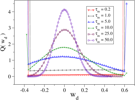
Figure 1: Distributions of the work done in driving a magnet at different rates when magnetic field is changed linearly.

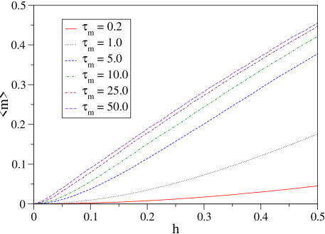
Figure 2: Average magnetization $m(\tau)$ for different rates, when magnetic field is changed linearly.

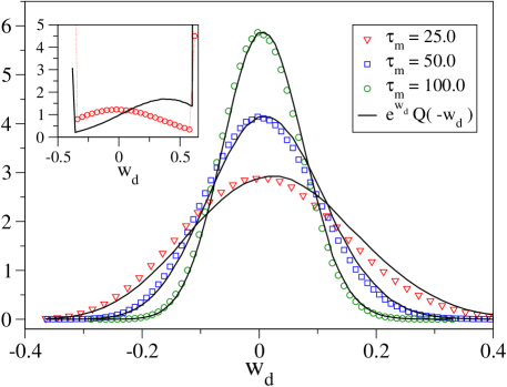
Figure 3: Plot shows that the fluctuation theorem is valid for slow processes with Gaussian work-distributions. Inset shows that for a fast rate ($\tau_{m}=5.0$) the probability of negative work is much larger than that predicted by the FT.

III.2 Field is taken around a cycle

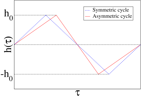
Figure 4: Magnetic field changed over a cycle. In the symmetric case the total cycle time is $4\tau_{m}$ while in the asymmetric case it is $2(\tau_{m}+\tau_{n})$.

As shown in Fig. 4 we consider two different cyclic forms for $f(\tau)$. One is a symmetric cycle and the other a asymmetric one. For these two cases the work-distributions are plotted in Fig. 5 and Fig. 6 respectively. For the symmetric cycle we plot the average magnetization as a function of the field in Fig. 7. This gives the familiar hysteresis curves.

As before we again find that the work-distributions are broad. For slow rates we get Gaussian distributions while for fast rates we get a $\delta-$function peak at the origin which correspond to a $0-$spin flip process. The slow and fast cases are treated analytically in section (III).

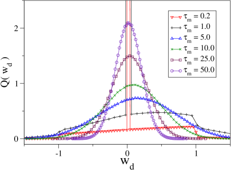
Figure 5: Plot of work-distributions for different driving rates when magnetic field is changed in a symmetric cycle.

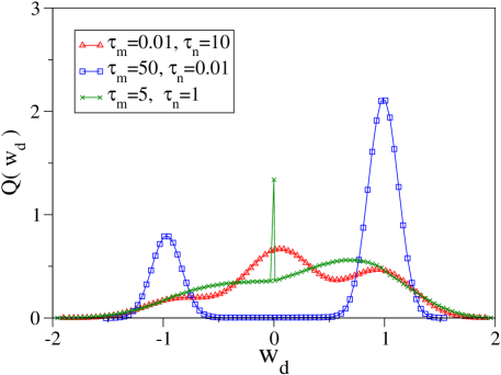
Figure 6: Plot of work-distributions obtained for different asymmetric cycles of the magnetic field.

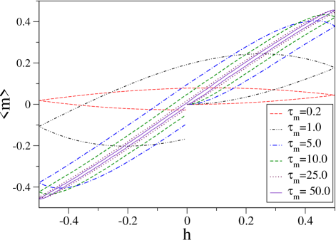
Figure 7: Hysteresis curves in driving a magnet at different rates when magnetic field is changed in a symmetric cycle and with the spin initially in equilibrium.

As expected we can verify the transient fluctuation theorem for both the symmetric and asymmetric processes. That TFT should be satisfied follows from Crooks FT and noting that the time reversed process has the same distribution as the forward process because of the additional $h\to-h$ symmetry that we have in this case.

We have also studied an asymmetric half-cycle for which $Q_{R}(w_{d})\neq Q(w_{d})$. Consequently we find that the usual TFT is not satisfied while the more general form of TFT of Crooks holds. We show this in Fig. 8 where we have plotted $Q(w_{d})$, $e^{w_{d}}Q(-w_{d})$ and $e^{w_{d}}Q_{R}(-w_{d})$.

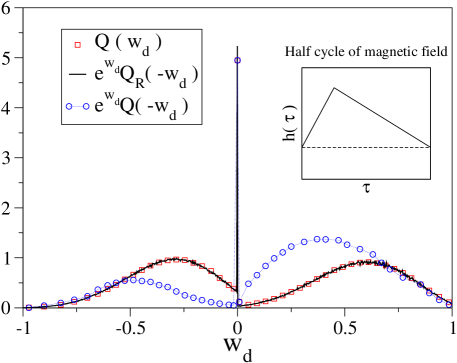
Figure 8: Plot showing the work-distribution for an asymmetric half-cycle and the validity of Crook’s fluctuation theorem. Note that the probability of negative work processes is much higher than that predicted by usual TFT.

III.3 Properties in the nonequilibrium steady state

We now look at the case when the spin is driven by the oscillating field into a nonequilibrium steady state and we measure fluctuations in this steady state. In this case the work distributions (over a cycle) have the same forms as in the transient case (Fig. 9).

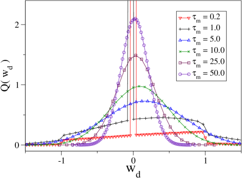
Figure 9: Work-distributions in the nonequilibrium steady state.

The joint distribution function $Q(w,\sigma,\tau)$ satisfies the same equation Eq. 18 but now the initial conditions are different. In Fig. 10 we plot the steady state hysteresis curves. Note that unlike the transient case the hysteresis curves are now closed loops.

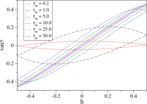
Figure 10: Hysteresis curves in the nonequilibrium steady state.

Finally we test the validity of the steady state fluctuation theorem (SSFT). This theorem has been proved for dynamical systems evolving through deterministic equations but there exists no proof that a similar result holds for stochastic dynamics. From Fig. 11 it is clear that SSFT does not hold.

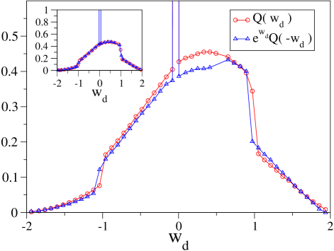
Figure 11: Violation of the fluctuation theorem for the steady state work-distribution corresponding to $\tau_{m}=0.5$. Inset shows the same plots for the transient case where FT is clearly satisfied.

IV Analytic results for slow and fast rates

IV.1 Field increased linearly from $0$ to $\epsilon$

(i) Slow case: $\tau_{m}>>1$

As argued in the previous section we expect that the work-distributions to be Gaussians which will be of the general form

$$Q(w)=\frac{1}{\sqrt{2\pi\sigma^{2}}}\ e^{\frac{-(w-\langle w\rangle)^{2}}{2\sigma_{w}^{2}}\ }\ .$$ (28)

Since the distribution satisfies Jarzynski’s equality, it follows at once that the mean and variance are related by

$$\sigma_{w}^{2}=2(\langle{w}\rangle-{\beta\Delta F}).$$ (29)

Hence we just need to find the mean work done. The mean work done is given by $\langle w\rangle=-(\epsilon/\tau_{m})\int_{0}^{\tau_{m}}d\tau m(\tau)$. In the strict adiabatic limit $\tau_{m}\to\infty$ we have $m_{ad}(\tau)=tanh(\epsilon\tau/\tau_{m})$ and the mean work done $\langle w\rangle=-\log(\cosh(\epsilon))=\beta\Delta F$. For large $\tau_{m}$ we try the perturbative solution

$$m(\tau)=m_{ad}(\tau)+\frac{1}{\tau_{m}}g(\tau)$$ (30)

Substituting in Eq. 15 we get an equation for $g(\tau)$ whose solution gives

$$g(\tau)=-(\epsilon)sech^{2}{(\frac{\epsilon\tau}{\tau_{m}})}+O(\frac{1}{\tau_{m}^{2}})$$ (31)

For the work done we then get

$$\langle w\rangle=\beta\Delta F+\frac{\epsilon}{\tau_{m}}tanh(\epsilon)$$ (32)

In Fig. 12 we compare the simulations for slow rates with the analytic results.

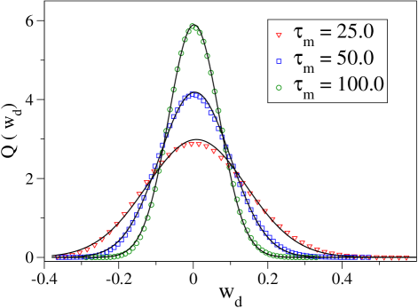
Figure 12: Comparison of work-distributions for slow rates obtained from simulations and from the analytic form. Solid lines show the analytic results.

(ii) Fast case: $\tau_{m}<<1$.

If we change the field very fast then the spin is not able to respond and so there are few spin flips during the entire process. At the lowest order there is no flip and this gives rise to the $\delta-$functions peaks at $\pm\epsilon$ seen in the distribution. We now calculate the work-distribution by looking at contributions from $0-$spin flip and $1-$spin flip processes. Let $S(\uparrow,\tau_{0},\tau)$ be the probability that, given that the spin is $\uparrow$ at time $\tau_{0}$, it remains in the same state till time $\tau$. It is easy to see that $S(\uparrow,\tau_{0},\tau)$ satisfies the equation

$$\frac{\partial S(\uparrow,\tau_{0},\tau)}{\partial\tau}\ =-\frac{e^{-\epsilon f(\tau)}}{Z}S(\uparrow,\tau_{0},\tau)$$ (33)

Solving we get, for the linear case $f(\tau)=\tau/\tau_{m}$,

$$S(\uparrow,0,\tau)=e^{-\int_{0}^{\tau}\frac{e^{-\epsilon\frac{\tau^{\prime}}{\tau_{m}}}}{Z(\tau^{\prime})}d\tau^{\prime}}=e^{\frac{-\tau}{2}}(\cosh(\frac{\epsilon\tau}{\tau_{m}}))^{\frac{\tau_{m}}{2\epsilon}}$$ (34)

Putting $\tau=\tau_{m}$ corresponds to the process for which the work done is $w=-\epsilon$. Hence, since the probability of the spin being initially in $\uparrow$ state is $1/2$, we get

$$Prob(w=-\epsilon)=\frac{1}{2}e^{-\frac{\tau_{m}}{2}}[\cosh(\epsilon)]^{\frac{\tau_{m}}{2\epsilon}}$$ (35)

Proceeding in a similar fashion by starting with a $\downarrow$ spin we get

$$Prob(w=\epsilon)=\frac{1}{2}\ e^{\frac{-\tau_{m}}{2}}(\cosh(\epsilon))^{-\frac{\tau_{m}}{2\epsilon}}$$ (36)

Next let us consider $1-$spin flip processes which (for fast rates) are the major contributors to the part of the distribution between the two peaks. Let $S_{1}(\uparrow,\tau)d\tau$ be the probability that the spin starts in the $\uparrow state$, flips once between times $\tau$ to $\tau+d\tau$, and stays $\downarrow$ till time $\tau_{m}$. This is given by

$$S_{1}(\uparrow,\tau)d\tau=S(\uparrow,0,\tau)(e^{-\epsilon\tau/\tau_{m}}/Z)d\tau S(\downarrow,\tau,\tau_{m})$$ (37)

The work done during such a process is given by

$$w=-\frac{\epsilon}{\tau_{m}}\ (2\tau-\tau_{m})$$ (38)

Similarly the case where the spin starts from a $\downarrow$ state gives

$$S_{1}(\downarrow,\tau)d\tau=S(\downarrow,0,\tau)(e^{\epsilon\tau/\tau_{m}}/Z)d\tau S(\uparrow,\tau,\tau_{m})$$ (39)

and the work done in this case is

$$w=\frac{\epsilon}{\tau_{m}}\ (2\tau-\tau_{m})$$ (40)

Adding this two contributions and plugging in the form of $S(\sigma,\tau_{0},\tau)$ obtained earlier we get the following contribution to the work-distribution:

$$Q_{1}(w)=\frac{\tau_{m}}{8\epsilon}e^{\frac{-(\tau_{m}-w)}{2}}(\frac{e^{\frac{-\epsilon}{2}}(\cosh(\epsilon)^{\frac{\tau_{m}}{2\epsilon}})}{\cosh(\frac{\epsilon-w}{2})}+\frac{e^{\frac{\epsilon}{2}}(\cosh(\epsilon)^{\frac{-\tau_{m}}{2\epsilon}})}{\cosh(\frac{\epsilon+w}{2})})$$

The full distribution is given by

$$Q(w) = \frac{1}{2}e^{-\frac{\tau_{m}}{2}}[\cosh(\epsilon)]^{\frac{\tau_{m}}{2\epsilon}}\delta(w+\epsilon)$$ (41)

$$+ \frac{1}{2}e^{-\frac{\tau_{m}}{2}}[\cosh(\epsilon)]^{-\frac{\tau_{m}}{2\epsilon}}\delta(w-\epsilon)+Q_{1}(w)$$

for $-\epsilon<w<\epsilon$, and zero elsewhere. In Fig. 13 we show a comparison of this analytic form with simulation results for $\tau_{m}=0.01$. The strengths of the $\delta-$functions at $w=\pm\epsilon$ are accurately given by Eqs. 35, 36.

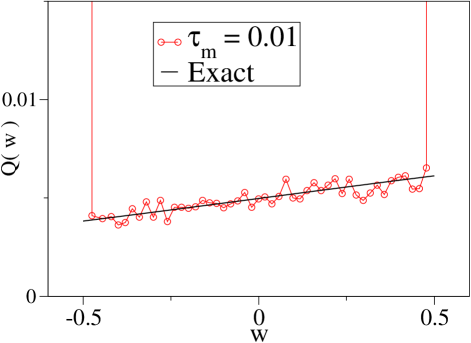
Figure 13: Comparison of work-distribution for a fast rate obtained from simulation and from the analytic form.

IV.2 Field is taken around a cycle

(i) Slow case: $\tau_{m}>>1$

We again expect a Gaussian distribution and since $\Delta F=0$ for a cyclic process, hence the mean and variance of the distribution are related by $\sigma_{w}^{2}=2\langle{w}\rangle$ (see Fig.14). As before we compute the mean work to order $1/\tau_{m}$ and find

$$\langle w\rangle=\frac{4\epsilon}{\tau_{m}}tanh(\epsilon)$$ (42)

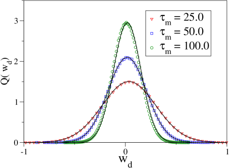
Figure 14: Comparison of work-distributions for slow rates obtained from simulations of the cyclic case and from the analytic form. Solid lines show the analytic results.

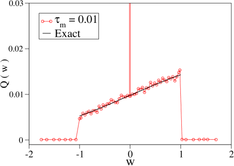
Figure 15: Comparison of work-distribution, for the symmetric cycle with a fast rate, obtained from simulations and from the analytic results.

(ii) Fast case: $\tau_{m}<<1$.

In this case the work distribution gives a $\delta-$function peak at the origin for $0-$spin flip processes. To find the probability of this, we solve Eq. 33 with $f(\tau)$ for the cycle given by

$$f(\tau) = \frac{\epsilon}{\tau_{m}}\tau~{}~{}~{}~{}~{}~{}~{}~{}~{}~{}~{}~{}~{}\text{for}\hskip 8.5359pt0\leq\tau\leq\tau_{m}$$

$$f(\tau) = \frac{\epsilon}{\tau_{m}}(2\tau_{m}-\tau)~{}~{}\text{for}\hskip 8.5359pt\tau_{m}\leq\tau\leq 3\tau_{m}$$

$$f(\tau) = \frac{\epsilon}{\tau_{m}}(\tau-4\tau_{m})~{}~{}\text{for}\hskip 8.5359pt3\tau_{m}\leq\tau\leq 4\tau_{m}$$

This has the solution

$$S(\uparrow,0,\tau_{m})=e^{-2\tau_{m}}$$ (43)

Adding up an equal contribution from $S(\downarrow,0,\tau_{m})$, and since both initial conditions occur with probability half, we finally get

$$Prob(w=0)=e^{-2\tau_{m}}$$ (44)

Next we look at the contribution of $1-$spin flip processes. Let the spin flip occur between times $\tau$ and $\tau+d\tau$. It is convenient to divide the total time $4\tau_{m}$ into four equal intervals, the dependence of $w$ on $\tau$ being different in each of the intervals. Thus if we start with the spin initially in an $\uparrow$ state then we have

$$w = -\frac{2\epsilon\tau}{\tau_{m}}~{}~{}~{}~{}~{}~{}~{}~{}~{}~{}~{}~{}~{}0<\tau<\tau_{m}$$

$$= \frac{2\epsilon}{\tau_{m}}(\tau-2\tau_{m})~{}~{}~{}\tau_{m}<\tau<2\tau_{m}$$

$$= \frac{2\epsilon}{\tau_{m}}(2\tau_{m}-\tau)~{}~{}~{}2\tau_{m}<\tau<3\tau_{m}$$

$$= \frac{2\epsilon}{\tau_{m}}(\tau-4\tau_{m})~{}~{}~{}3\tau_{m}<\tau<4\tau_{m}.$$

The probabilities of each of these processes is again given by:

$$S_{1}(\uparrow,\tau)d\tau=S(\uparrow,0,\tau)(e^{-\epsilon f(\tau)}/Z)d\tau S(\downarrow,\tau,4\tau_{m})$$ (45)

Using the relations between $w$ and $\tau$ and summing up the four different possibilities we finally get (for initial spin state $\uparrow$)

$$Q_{1}^{\uparrow}(w) = \frac{\tau_{m}}{8\epsilon}e^{-2\tau_{m}}e^{\frac{w}{2}}[(\cosh(\frac{w}{2}))^{\frac{\tau_{m}}{\epsilon}-1}$$ (46)

$$+ (\cosh(\frac{w}{2}))^{-\frac{\tau_{m}}{\epsilon}-1}(\cosh(\epsilon))^{\frac{2\tau_{m}}{\epsilon}}]$$

for $-1<w<1$ and zero elsewhere. Note that the allowed range of $w$ is $[-2,2]$ but single spin-flip processes only contribute to work in the range $[-1,1]$. Similarly if we start with spin state $\downarrow$ we get

$$Q_{1}^{\downarrow}(w) = \frac{\tau_{m}}{8\epsilon}e^{-2\tau_{m}}e^{\frac{w}{2}}[(\cosh(\frac{w}{2}))^{-\frac{\tau_{m}}{\epsilon}-1}$$ (47)

$$+ (\cosh(\frac{w}{2}))^{\frac{\tau_{m}}{\epsilon}-1}(\cosh(\epsilon))^{-\frac{2\tau_{m}}{\epsilon}}]$$

for $-1<w<1$. The full work-distribution (contribution from $1-$spin flip processes) is thus:

$$Q(w)=e^{-2\tau_{m}}\delta(w)+Q_{1}^{\uparrow}(w)+Q_{1}^{\downarrow}(w)$$ (48)

In Fig. 15 we compare the analytic and simulation results. The strength of the $\delta-$function at $w=0$ is accurately given by Eq. 44.

V Discussion

We have computed probability distributions of the work done when a single spin, with Markovian dynamics, is driven by a time dependent magnetic field. We find that work fluctuations are quite large (even for slow driving rates) and there is significant probability for processes with negative dissipated work. For slow driving the number of spin flips during the entire process is very large and the total work is effectively a sum of random variables. Hence the distributions are Gaussian with widths proportional to the driving rate. On the other hand for very fast driving the probability of flipping is low and we can compute the work-distributions perturbatively from probabilities of zero-flip, one-flip, etc. processes.

While the two special cases of slow and fast rates can be solved, it looks difficult to obtain a general solution valid for all rates even in this single particle problem. We note that the problem of calculating the work-distribution is similar to that of calculating residence-time distributions in stochastic processes dornic ; newman ; satya . In fact for the case in section(IIIA) the work done is proportional to the average magnetization which is easily related to the residence time (time spin spends in $\uparrow$ state). For stationary stochastic processes, such as the random walk, the residence time distribution can be obtained exactly. However for non-stationary processes this becomes difficult and no exact solutions are available satya . In our spin-problem too it appears that the non-stationarity of the process makes an exact solution difficult.

For a system with $N$ spins the total work done on the system is simply a sum of the work done on each of the spins. For the case where the spins are non-interacting we thus get a sum of $N$ independent random variables. For large $N$ the distribution will be a Gaussian with a mean that scales with $N$ and variance as $N^{1/2}$. For interacting spins the properties of the work-distribution is an open problem. Especially of interest is the question as to what happens as we cross the transition temperature. Finally we note that the large fluctuations in the area under a hysteresis curve should be experimentally observable in nano-scale magnets.

- (1) C. Bustamante, J. Liphardt and F. Ritort, Physics Today 58(7), p.43, (July 2005).
- (2) M. J. Perrin, Brownian Movement and Molecular Reality, page 6 (Taylor and Francis, London, 1910).
- (3) C. Jarzynski, Phys. Rev. Lett. 78, 2690 (1997); C. Jarzynski, Phys. Rev. E 56, 5018 (1997).
- (4) E. G. D. Cohen, D. Mauzerall, J. Stat. Mech. P07006 (2004); C. Jarzynski, J. Stat. Mech: Theor. Exp. P09005 (2004).
- (5) D. J. Evans, E G. D. Cohen, and G. P. Morriss, Phys. Rev. Lett. 71, 2401 (1993); D. J. Evans and D. J. Searles, Phys. Rev. E 50, 1645 (1994); G. Gallavotti and E. G. D. Cohen, Phys. Rev. Lett. 74, 2694 (1995).
- (6) G. E. Crooks, Phys. Rev. E 60, 2721 (1999).
- (7) J. Kurchan, J. Phys. A: Math. Gen. 31, 3719 (1998); J. L. Lebowitz and H. Spohn, J. Stat. Phys. 95, 333 (1999).
- (8) O. Narayan and A. Dhar, J. Phys. A: Math. Gen. 37 63 (2004).
- (9) R. van Zon and E. G. D. Cohen, Phys. Rev. Lett. 91, 110601 (2003); R. van Zon, S. Ciliberto and E. G. D. Cohen, Phys. Rev. Lett. 92, 130601 (2004).
- (10) J. Liphardt et al, Science 296, 1832 (2002);
- (11) G. M. Wang et al, Phys. Rev. Lett. 89, 050601 (2002);
- (12) K. Feitosa and N. Menon, Phys. Rev. Lett. 92, 164301 (2004); S. Aumaître et al, Eur. Phys. J. B 19, 449 (2001); W. I. Goldburg, Y. Y. Goldschmidt and H. Kellay, Phys. Rev. Lett. 87, 245502 (2001); N. Garnier and S. Ciliberto, Phys. Rev E 71, 060101(R) (2005).
- (13) F. Douarche et al, Europhys. Lett., 70(5), p.593, (2005)
- (14) G. Hummer and A. Szabo, Proc. Natl. Acad. Sci 98, 3658 (2001); J. Gore, F. Ritort and C. Bustamante, Proc. Natl. Acad. Sci. 100, 12564 (2003); R. F. Fox, Proc. Natl. Acad. Sci. 100, 12537 (2003); S. Park et al, J. Chem. Phys. 119, 3559 (2003).
- (15) T. Tom and M. J. de Oliveira, Phys. Rev. A 41, 4251 (1990); M. Rao, H. Krishnamurthy and R. Pandit, Phys. Rev. B 42, 856 (1990); B. Chakrabarti and M. Acharyya, Rev. Mod. Phys. 71, 847 (1999).
- (16) S. W. Sides, P. A. Rikvold, and M. A. Novotny, Phys. Rev. E 57, 6512 (1998)
- (17) F. Ritort, C. Bustamante and I. Tinoco Jr., Proc. Natl. Acad. Sci. 99, 13544 (2002).
- (18) A. Imparato and L. Peliti, Europhys. Lett., 69, 643 (2005).
- (19) T. Speck and U. Seifert, Phys. Rev. E 70, 066112 (2004).
- (20) A. Dhar, Phys. Rev. E 71, 36126 (2005).
- (21) I. Dornic and C. Godr che, J. Phys. A 31, 5413 (1998).
- (22) T.J. Newman and Z. Toroczkai, Phys. Rev. E 58, R2685 (1998).
- (23) A. Dhar and S. N. Majumdar, Phys. Rev. E 59, 6413 (1999).