Width of Percolation Transition in Complex Networks

Abstract

It is known that the critical probability for the percolation transition is not a sharp threshold, actually it is a region of non-zero width $\Delta p_{c}$ for systems of finite size. Here we present evidence that for complex networks $\Delta p_{c}\sim\frac{p_{c}}{l}$, where $l\sim N^{\nu_{opt}}$ is the average length of the percolation cluster, and $N$ is the number of nodes in the network. For Erdős-Rényi (ER) graphs $\nu_{opt}=1/3$, while for scale-free (SF) networks with a degree distribution $P(k)\sim k^{-\lambda}$ and $3<\lambda<4$, $\nu_{opt}=(\lambda-3)/(\lambda-1)$. We show analytically and numerically that the survivability $S(p,l)$, which is the probability of a cluster to survive $l$ chemical shells at probability $p$, behaves near criticality as $S(p,l)=S(p_{c},l)\cdot exp[(p-p_{c})l/p_{c}]$. Thus for probabilities inside the region $|p-p_{c}|<p_{c}/l$ the behavior of the system is indistinguishable from that of the critical point.

I Introduction:

Recently the subject of networks has received much attention. It was realized that many systems in the real world, such as the Internet, can be successfully modeled as networks. Other examples include social networks such as the web of social contacts, and biological networks such as the protein interaction network and metabolic networks Barabási (2002); Dorogovtsev and Mendes (2003); Pastor-Satorras and Vespignani (2004). The problem of percolation on networks has also been studied extensively (e.g. Albert and Barabási (2002)). Using percolation theory we can describe the resilience of the network to breakdown of sites or links Callaway et al. (2000); Cohen et al. (2000), epidemic spreading Cohen et al. (2003), and the properties of the optimal path in a highly network with highly fluctuating weights on the links Braunstein et al. (2003).

A typical percolation system consists of a $d$-dimensional grid of length $L$, in which the nodes or links are removed with some probability $1-p$, or are considered “conducting” with probability $p$ (e.g. Bunde and Havlin (1996); Stauffer and Aharony (1992)). Below some critical probability $p_{c}$ the system becomes disconnected into small clusters, i.e., it becomes impossible to cross from one side of the grid to the other by following the conducting links. Percolation is considered a geometrical phase transition exhibiting universality, critical exponents, upper critical dimension at $d=6$ etc. It was noted by Conigilio Coniglio (1982) that for systems of finite size $L$ the transition from connected to disconnected state has a width $\Delta p_{c}\sim\frac{1}{L^{1/\nu}}$, where $\nu$ is a critical exponent related to the correlation length.

Percolation on networks was studied also from a mathematical point of view Erdös and Rényi (1960); Bollobás (2001); Albert and Barabási (2002). It was found that in Erdős-Rényi (ER) graphs with an average degree $\langle k\rangle$ the percolation threshold is: $p_{c}=\frac{1}{\langle k\rangle}$. Below $p_{c}$ the graph is composed of small clusters (most of them trees). As $p$ approaches $p_{c}$ trees of increasing order appear. At $p=p_{c}$ a giant component emerges and loops of all orders abruptly appear. Nevertheless, for graphs of finite size $N$ it was found that the percolation threshold has a finite width $\Delta p_{c}\sim\frac{1}{N^{1/3}}$ Bollobás (2001), meaning that all attributes of criticality are present in the system in the range $[p_{c}-\Delta p_{c},p_{c}+\Delta p_{c}]$. For example: The number of loops is negligible below $p_{c}+\Delta p_{c}$ .

In this paper we study the Survivability of the network near the critical threshold. The survivability $S(p,l)$ is defined to be the probability of a connected cluster to “survive” up to $l$ chemical shells in a system with conductance probability $p$ Tzschichholz et al. (1989) (i.e the probability that there exists at least one node at chemical distance $l$ from a randomly chosen node on the same cluster). At the critical point $p_{c}$, the survivability decays as a power-law: $S(p_{c},l)\sim l^{-x}$, where $x$ is a universal exponent. Below $p_{c}$ the survivability decays exponentially to zero, while above $p_{c}$ it decays (exponentially) to a constant. Here we will derive analytically and numerically the functional form of the survivability above and below the critical point. We will show that near the critical point $S(p,l)=S(p_{c},l)\cdot exp[(p-p_{c})l/p_{c}]$. Thus, given a system with a maximal chemical length $l$, for probabilities inside the range $|p-p_{c}|<\frac{p_{c}}{l}$ the behavior of the system is indistinguishable from that of the critical point. Hence we get $\Delta p_{c}\sim\frac{p_{c}}{l}$.

The maximal chemical length $l$ at criticality is actually the length of the percolation cluster, which was found to be: $l\sim N^{\nu_{opt}}$ where $N$ is the number of nodes in the network. For Erdős-Rényi (ER) graphs $\nu_{opt}=1/3$, while for scale-free (SF) networks with a degree distribution $P(k)\sim k^{-\lambda}$ and $3<\lambda<4$, $\nu_{opt}=(\lambda-3)/(\lambda-1)$ Braunstein et al. (2003).

II Erdős-Rényi Graphs:

Consider an ER graph with a mean degree $\langle k\rangle$, and each link having a probability $p$ to conduct. We define $N_{l}(x)=n_{0}+n_{1}x+n_{2}x^{2}+n_{3}x^{3}+...$ to be the generating function of the number of sites that exists on layer (i.e. chemical shell) $l$ starting from a random node on the graph (for a conduction probability $p$).

The generating function for the degree distribution of a randomly chosen node in the network is $G_{0}(x)=\sum P(k)\cdot x^{k}$ and the generating function for the number of links emerging from a node reached by following a randomly chosen link is $G_{1}(x)=\Sigma\frac{1}{\langle k\rangle}kP(k)\cdot x^{k-1}$ Newman et al. (2001). Taking into account the probability $p$ for conduction, we have:

$$G_{1}(x)=1-p+p\sum\frac{1}{\langle k\rangle}kP(k)\cdot x^{k-1}.$$ (1)

We can now write the following recursive relation Kalisky et al. (2004):

$$N_{l+1}(x)=G_{1}(N_{l}(x)),$$ (2)

which means that the probability $n^{(l+1)}_{i}$ for having $i$ nodes at layer $l+1$ is composed of the probability of reaching a vertex by following a link, and reaching $i$ nodes at layer $l$ by following all branches emerging from that vertex - see sketch in Fig. 1.

It can be seen that $N_{l}(0)=n_{0}$ is the probability that there are $0$ nodes at layer $l$, i.e., the probability to die before layer $l$. Thus $\epsilon_{l}=1-N_{l}(0)$ is the probability to survive up to layer $l$. From (2) we have:

$$N_{l+1}(0)=G_{1}(N_{l}(0))$$ (3)

$$1-\epsilon_{l+1}=G_{1}(1-\epsilon_{l})$$ (4)

$$1-\epsilon_{l+1}=1-p+p\sum\frac{1}{\langle k\rangle}kP(k)(1-\epsilon_{l})^{k-1}$$ (5)

For ER graphs $G_{0}(x)=G_{1}(x)=e^{{\langle k\rangle(x-1)}}$ (for $p=1$), Thus:

$$1-\epsilon_{l+1}=1-p+pe^{\langle k\rangle(1-\epsilon_{l}-1)}=1-p+pe^{-\langle k\rangle\epsilon_{l}}$$ (6)

$$\epsilon_{l+1}=p-pe^{-\langle k\rangle\epsilon_{l}}$$ (7)

Setting $\delta\equiv p-p_{c}$, where $p_{c}=\frac{1}{\langle k\rangle}$, and expanding by series we get:

$$\epsilon_{l+1}=p_{c}+\delta-(p_{c}+\delta)\left(1-\langle k\rangle\epsilon_{l}+\frac{1}{2}\langle k\rangle^{2}\epsilon_{l}^{2}-...\right)$$ (8)

Leaving only expressions up to second order in $\delta$ and $\epsilon_{l}$ (we assume that $p<p_{c}$ and thus $\epsilon_{l}\ll 1$ for large $l$) we get:

$$\epsilon_{l+1}\approx\epsilon_{l}-\frac{1}{2}\langle k\rangle\epsilon_{l}^{2}+\delta\langle k\rangle\epsilon_{l}$$ (9)

$$\frac{d\epsilon_{l}}{dl}\approx-\frac{1}{2}\langle k\rangle\epsilon_{l}^{2}+\frac{\delta}{p_{c}}\cdot\epsilon_{l}$$ (10)

At criticality, $\delta=0$ and the solution to this equation is: $\epsilon_{l}\sim l^{-1}$ Kalisky et al. (2004). The additional term suggests the following solution near criticality: $\epsilon_{l}\sim l^{-1}\cdot\exp{\left(\frac{1}{p_{c}}\delta l\right)}$ .

In terms of survivability this can be written as:

$$S(p,l)=S(p_{c},l)\cdot\exp\left(\frac{1}{p_{c}}(p-p_{c})l\right).$$ (11)

In order to check this result we numerically solved the survivability $S(p,l)$ near $p_{c}$ according to the exact enumeration method presented in Braunstein et al. (2004) . Fig. 2 shows the survivability $S(p,l)$ for different values of $p$. For $p=p_{c}$ the survivability decays as a power law, while above and below there is an exponential decay, either to zero (for $p<p_{c}$) or to a constant (for $p>p_{c}$). Fig. 3 shows that all curves of the survivability $S(p,l)$ from Fig. 2 can be rescaled such that they all collapse. Moreover, scaled survivabilities from all different graphs with different values of $\langle k\rangle$ (i.e., different values of $p_{c}$) also collapse on the same curve. However, equation (11) is true only below the percolation threshold where there is no giant component. Above the percolation threshold there is an exponential decay to a non-zero constant, and the generalized expression is:

$$S(p,l)=S(p_{c},l)\cdot\exp\left(-\frac{1}{p_{c}}|p-p_{c}|l\right)+pP_{\infty},$$ (12)

Where $pP_{\infty}$ is the probability for a randomly chosen site to be inside the percolation cluster . Indeed, setting $\epsilon_{l+1}=\epsilon_{l}$ in equation (7) the resulting “steady state” solution is $pP_{\infty}$ Bollobás (2001).

III Scale-Free Graphs:

Scale-free graphs can be taken to have a degree distribution of the form $P(k)=ck^{-\lambda}$ where $c\approx(\lambda-1)m^{\lambda-1}$ Cohen et al. (2000). In order to solve equation (5) we have to evaluate:

$$G_{1}(1-\epsilon_{l})=\frac{1}{\langle k\rangle}\sum kP(k)(1-\epsilon_{l})^{k-1}$$ (13)

Expanding by powers of $\epsilon_{l}$, and inserting $P(k)=ck^{-\lambda}$ with $3<\lambda<4$, we get Cohen and Havlin (2005):

$$\sum kP(k)(1-\epsilon_{l})^{k-1}\approx\langle k\rangle-\langle k(k-1)\rangle\epsilon_{l}+\frac{c}{2}\Gamma(4-\lambda)\epsilon_{l}^{\lambda-2}$$ (14)

Thus equation (5) becomes:

$$1-\epsilon_{l+1}\approx 1-p+\frac{p}{\langle k\rangle}\left(\langle k\rangle-\langle k(k-1)\rangle\epsilon_{l}+\frac{c}{2}\Gamma(4-\lambda)\epsilon_{l}^{\lambda-2}\right)$$ (15)

Taking $p=p_{c}+\delta$:

$$1-\epsilon_{l+1}\approx 1-(p_{c}+\delta)+\frac{p_{c}+\delta}{\langle k\rangle}\left(\langle k\rangle-\langle k(k-1)\rangle\epsilon_{l}+\frac{c}{2}\Gamma(4-\lambda)\epsilon_{l}^{\lambda-2}\right).$$ (16)

Substituting $p_{c}=\frac{\langle k\rangle}{\langle k(k-1)\rangle}$ Cohen et al. (2000) we get:

$$1-\epsilon_{l+1}\approx 1-\epsilon_{l}+p_{c}\frac{c}{2\langle k\rangle}\Gamma(4-\lambda)\cdot\epsilon_{l}^{\lambda-2}-\frac{1}{p_{c}}\cdot\delta\epsilon_{l}+\frac{c}{2\langle k\rangle}\Gamma(4-\lambda)\cdot\delta\epsilon_{l}^{\lambda-2}$$ (17)

Setting $A\equiv p_{c}\frac{c}{2\langle k\rangle}\Gamma(4-\lambda)$ we get:

$$\epsilon_{l+1}-\epsilon_{l}\approx-A\cdot\epsilon_{l}^{\lambda-2}+\frac{1}{p_{c}}\cdot\delta\epsilon_{l}-\frac{A}{p_{c}}\cdot\delta\epsilon_{l}^{\lambda-2}$$ (18)

$$\epsilon_{l+1}-\epsilon_{l}\approx-A\cdot\epsilon_{l}^{\lambda-2}+\frac{1}{p_{c}}\cdot\delta\left(\epsilon_{l}-A\cdot\epsilon_{l}^{\lambda-2}\right).$$ (19)

For large $l$, $\epsilon_{l}\ll 1$, and taking into account that $\lambda-2>1$ we have $\epsilon_{l}^{\lambda-2}\ll\epsilon_{l}$. Therefore:

$$\frac{d\epsilon_{l}}{dl}\approx-A\cdot\epsilon_{l}^{\lambda-2}+\frac{1}{p_{c}}\cdot\delta\epsilon_{l}.$$ (20)

For $\delta=0$ the solution is $\epsilon_{l}\sim l^{-x}$ with $x=\frac{1}{\lambda-3}$ Kalisky et al. (2004). The additional term suggests the following solution near criticality: $\epsilon_{l}\sim l^{-x}\cdot\exp{\left(\frac{\delta l}{p_{c}}\right)}$ . A similar form can be found for $\lambda>4$ . The scaling form for SF networks is also confirmed by numerical simulations as shown in Figures 4 and 5.

IV Summary and Conclusions

The scaling form of the survivability near the critical probability obeys the following scaling relation (for $p<p_{c}$):

$$S(p,l)=S(p_{c},l)\cdot\exp\left(\frac{p-p_{c}}{\Delta p_{c}}\right).$$ (21)

Where $\Delta p_{c}=\frac{p_{c}}{l}$. Given a system with a maximal chemical length $l$, for all values of conductivity $p$ inside the range $[p_{c}-\Delta p_{c},p_{c}+\Delta p_{c}]$ the survivability behaves similar to the power law $S(p_{c},l)\sim l^{-x}$ found at criticality. Thus, the width of the critical threshold is $\Delta p_{c}=\frac{p_{c}}{l}$.

To summarize, we have shown analytically and numerically the the survivability in ER and SF graphs scales according to equations (11) and (12) near the critical point. This implies that the width of the critical region in networks of finite size scales as $\Delta p_{c}=\frac{p_{c}}{l}$, where $l$ is the chemical length of the percolation cluster. For ER graphs, $l\sim N^{1/3}$, while for SF networks with $3<\lambda<4$, $l\sim N^{(\lambda-3)/(\lambda-1)}$.

Figure 1: A graphical sketch of the recursion relation (2). Given a certain conduction probability $p$, the probability to reach $i$ nodes at layer $l+1$ is found by summing up the probabilities to follow a link to a node (whose outgoing degree is described by $G_{1}(x)$) and reaching $i$ nodes at layer $l$ from that node.

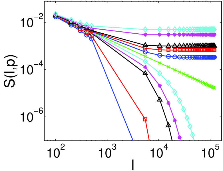
Figure 2: (Color online) The survivability $S(p,l)$ for an ER graphs with $\langle k\rangle=5$, numerically calculated for different values of $p$: $p_{c}$, $p_{c}\pm 5\cdot 10^{-4}$, $p_{c}\pm 3\cdot 10^{-4}$, $p_{c}\pm 1\cdot 10^{-4}$, $p_{c}\pm 6.66\cdot 10^{-5}$, and $p_{c}\pm 3.33\cdot 10^{-5}$. For $p=p_{c}$ the survivability decays to zero according to a power law: $S(p_{c},l)\sim l^{-1}$. For $p<p_{c}$, $S(p,l)\rightarrow 0$, while for $p>p_{c}$, $S(p,l)\rightarrow Const$. The decay is exponential (to zero or to a constant) according to equations (11) and (12).

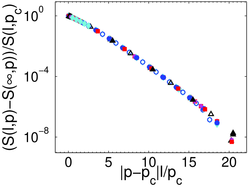
Figure 3: (Color online) Scaling of the survivability for different values of $p$, $l$, and $\langle k\rangle$. Shown is $\frac{S(p,l)-S(p,\infty)}{S(p_{c},l)}$ vs. $\frac{1}{p_{c}}|p-p_{c}|l$ for ER graphs with $\langle k\rangle=5$ (unfilled symbols) and $\langle k\rangle=10$ (filled symbols). The collapse of all curves on an exponential function (for large $l$) shows that indeed the scaling relations (11) and (12) are correct.

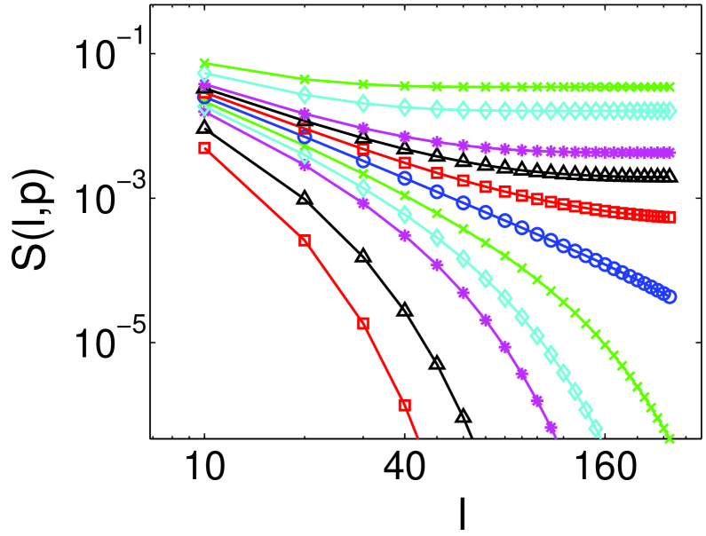
Figure 4: (Color online) The survivability $S(p,l)$ for a SF network with $\lambda=3.5$, numerically calculated for different values of $p$: $p_{c}$, $p_{c}\pm 6\cdot 10^{-2}$, $p_{c}\pm 4\cdot 10^{-2}$, $p_{c}\pm 2\cdot 10^{-2}$, $1.33\cdot 10^{-2}$, and $p_{c}\pm 6.66\cdot 10^{-3}$. For $p=p_{c}$ the survivability decays to zero according to a power law: $S(p_{c},l)\sim l^{-2}$. For $p<p_{c}$, $S(p,l)\rightarrow 0$, while for $p>p_{c}$, $S(p,l)\rightarrow Const$. The decay is exponential (to zero or to a constant) according to equations (11) and (12).

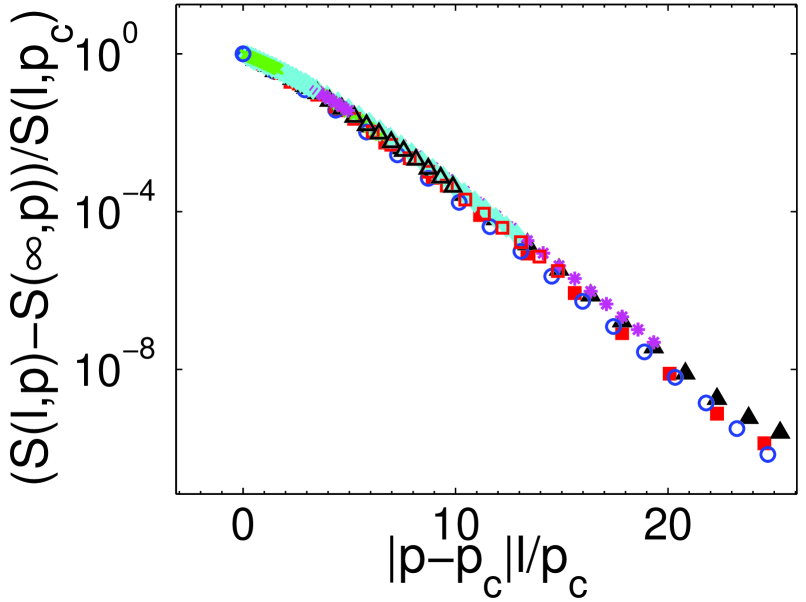
Figure 5: (Color online) Scaling of the survivability for different values of $p$, $l$, and $\lambda$. Shown is $\frac{S(p,l)-S(p,\infty)}{S(p_{c},l)}$ vs. $\frac{1}{p_{c}}|p-p_{c}|l$ for SF graphs with $\lambda=3.5$ (filled symbols) and $\lambda=5$ (unfilled symbols). Due to numerical difficulties only curves with $p<p_{c}$ are shown . All curves collapse on an exponential function according to relation (11).

References

- Barabási (2002) A.-L. Barabási, Linked: The new science of networks (Perseus Books Group, 2002).
- Dorogovtsev and Mendes (2003) S. N. Dorogovtsev and J. F. F. Mendes, Evolution of Networks - From Biological Nets to the Internet and WWW (Oxford University Press, 2003).
- Pastor-Satorras and Vespignani (2004) R. Pastor-Satorras and A. Vespignani, Evolution and Structure of the Internet : A Statistical Physics Approach (Cambridge University Press, 2004).
- Albert and Barabási (2002) R. Albert and A.-L. Barabási, Rev. of Mod. Phys. 74, 47 (2002).
- Callaway et al. (2000) D. S. Callaway, M. E. J. Newman, S. H. Strogatz, and D. J. Watts, Phys. Rev. Lett. 85, 5468 (2000).
- Cohen et al. (2000) R. Cohen, K. Erez, D. ben Avraham, and S. Havlin, Phys. Rev. Lett. 85, 4626 (2000).
- Cohen et al. (2003) R. Cohen, , and D. ben Avraham S. Havlin, Phys. Rev. Lett. 90, 247901 (2003).
- Braunstein et al. (2003) L. A. Braunstein, S. V. Buldyrev, R. Cohen, S. Havlin, and H. E. Stanley, Phys. Rev. Lett. 91, 168701 (2003).
- Bunde and Havlin (1996) A. Bunde and S. Havlin, eds., Fractals and Disordered Systems (Springer, New York, 1996).
- Stauffer and Aharony (1992) D. Stauffer and A. Aharony, Introduction to Percolation Theory (Taylor and Francis, London, 1992).
- Coniglio (1982) A. Coniglio, J. Phys. A. 15, 3829 (1982).
- Erdös and Rényi (1960) P. Erdös and A. Rényi, Publ. Math. Inst. Hungar. Acad. Sci. 5, 17 (1960).
- Bollobás (2001) B. Bollobás, Random Graphs (Cambridge University Press, 2001).
- Tzschichholz et al. (1989) F. Tzschichholz, A. Bunde, and S. Havlin, Phys. Rev. A 39, 5470 (1989).
- Newman et al. (2001) M. E. J. Newman, S. H. Strogatz, and D. J. Watts, Phys. Rev. E 64, 026118 (2001).
- Kalisky et al. (2004) T. Kalisky, R. Cohen, D. ben Avraham, and S. Havlin, in Lecture Notes in Physics: Proceedings of the 23rd LANL-CNLS Conference, ”Complex Networks”, Santa-Fe, 2003, edited by E. Ben-Naim, H. Frauenfelder, and Z. Toroczkai (Springer, Berlin, 2004).
- Braunstein et al. (2004) L. A. Braunstein, S. V. Buldyrev, S. Sreenivasan, R. Cohen, S. Havlin, and H. E. Stanley, in Lecture Notes in Physics: Proceedings of the 23rd LANL-CNLS Conference, ”Complex Networks”, Santa-Fe, New Mexico, May 12 - 16, 2003, edited by E. Ben-Naim, H. Frauenfelder, and Z. Toroczkai (Springer, Berlin, 2004).
- Cohen and Havlin (2005) R. Cohen and S. Havlin, Complex Networks: Structure, Stablity and Function (Cambridge University Press, to appear, 2005).
- Cohen et al. (2002) R. Cohen, D. ben Avraham, and S. Havlin, Phys. Rev. E 66, 036113 (2002).