Scaling of Optimal Path Lengths Distribution in Complex Networks

Abstract

We study the distribution of optimal path lengths in random graphs with random weights associated with each link (“disorder”). With each link $i$ we associate a weight $\tau_{i}=\exp(ar_{i})$ where $r_{i}$ is a random number taken from a uniform distribution between 0 and 1, and the parameter $a$ controls the strength of the disorder. We suggest, in analogy with the average length of the optimal path, that the distribution of optimal path lengths has a universal form which is controlled by the expression $\frac{1}{p_{c}}\frac{\ell_{\infty}}{a}$, where $\ell_{\infty}$ is the optimal path length in strong disorder ($a\rightarrow\infty$) and $p_{c}$ is the percolation threshold. This relation is supported by numerical simulations for Erdős-Rényi and scale-free graphs. We explain this phenomenon by showing explicitly the transition between strong disorder and weak disorder at different length scales in a single network.

I Introduction:

Many real world systems exhibit a web-like structure and may be treated as “networks”. Examples may be found in physics, sociology, biology, and engineering Albert and Barabási (2002); Dorogovtsev and Mendes (2003); Pastor-Satorras and Vespignani (2004). The function of most real world networks is to connect distant nodes, either by transfer of information (e.g. the Internet), or through transportation of people and goods (such as networks of roads and airlines). In many cases there is a “cost” or a “weight” associated with each link, and the larger the weight on a link, the harder it is to traverse this link. In this case, the network is called “disordered” or “weighted” Braunstein et al. (2003); Barrat et al. (2004). For example, in the Internet each link between two routers has a bandwidth or delay time, in a transportation network some roads may have only one lane while others may be highways allowing for large volumes of traffic.

The average length of the optimal path (or “shortest path”) in weighted lattices and networks has been extensively studied Cieplak et al. (1994, 1996); Porto et al. (1997); Braunstein et al. (2003); Sreenivasan et al. (2004). In weighted networks it is commonly assumed that each link is associated with a weight $\tau_{i}=\exp(ar_{i})$, where $r_{i}$ is a random number taken from a uniform distribution between 0 and 1, and the parameter $a$ controls the strength of the disorder. It has been shown Sreenivasan et al. (2004) that the length of the optimal path in such weighted networks scales as $l(a)\sim N^{\nu_{opt}}$ (where $\nu_{opt}$ is universal exponent) for small system size $N$, and $l(a)\sim\log{N}$ for large systems . More precisely:

$$\ell(a)\sim\ell_{\infty}F\left(\frac{\ell_{\infty}}{ap_{c}}\right),$$ (1)

where $p_{c}$ is the percolation threshold and $\ell_{\infty}\sim N^{\nu_{opt}}$ is the optimal path length for strong disorder ($a\rightarrow\infty$). For Erdős-Rényi (ER) graphs $\nu_{opt}=1/3$. For scale-free (SF) networks, with a power law degree distribution $P(k)\sim k^{-\lambda}$, $\nu_{opt}=(\lambda-3)/(\lambda-1)$ for $3<\lambda<4$ and $\nu_{opt}=1/3$ for $\lambda\geq 4$ Braunstein et al. (2003). The function $F(u)$ is of the form:

$$F(u)=\left\{\begin{array}[]{l c c}\mathrm{const}&\ \ \mathrm{if}&u\ll 1\\ \log(u)/u&\ \ \mathrm{if}&u\gg 1\end{array}\right..$$ (2)

In this paper we study the following question: how are the different optimal paths in a network distributed? The distribution of the optimal path lengths is especially important in communication networks, in which the overall network performance depends on the different path lengths between all nodes of the network, and not only the average. A recent work has studied the distribution form of shortest path lengths on minimum spanning trees Braunstein et al. (2004), which correspond to optimal paths on networks with large variation in link weights ($a\rightarrow\infty$).

We generalize these results and suggest that the distribution of the optimal path lengths has the following scaling form:

$$P(\ell,N,a)\sim\frac{1}{\ell_{\infty}}G\left(\frac{\ell}{\ell_{\infty}},\frac{1}{p_{c}}\frac{\ell_{\infty}}{a}\right).$$ (3)

The parameter $Z\equiv\frac{1}{p_{c}}\frac{\ell_{\infty}}{a}$ determines the functional form of the distribution. Relation (3) is supported by simulations for both ER and SF graphs, including SF graphs with $2<\lambda<3$, for which $p_{c}\rightarrow 0$ with system size $N$ Cohen et al. (2000) (Section II).

The paper is organized as follows: in Section II we show results from simulations for various ER and SF graphs. In Section III we explain these results and also show that the optimal path $l_{opt}(a)$ inside a single network scales differently below and above a characteristic length $\xi=ap_{c}$. For $\ell<\xi$ it is like strong disorder, while for $\ell>\xi$ the behavior is like weak disorder.

II Erdős-Rényi and Scale-Free Graphs:

We simulate ER graphs with weights on the links for different values of graph size $N$, control parameter $a$, and average degree $\langle k\rangle$ (which determines $p_{c}=1/\langle k\rangle$) – see Table 1. We then generate the shortest path tree (SPT) using Dijkstra’s algorithm Cormen et al. (2001) from some randomly chosen root node. Next, we calculate the probability distribution function of the shortest (i.e. optimal) path lengths for all nodes in the graph.

In Fig. 1 we plot $\ell_{\infty}P(\ell,N,a)$ vs. $\ell/\ell_{\infty}$ for different values of $N$, $a$, and $\langle k\rangle$. A collapse of the curves is seen for all graphs with the same value of $Z=\frac{1}{p_{c}}\frac{\ell_{\infty}}{a}$.

Figure 2 shows similar plots for SF graphs – with a degree distribution of the form $P(k)\sim k^{-\lambda}$ and with a minimal degree $m$  . A collapse is obtained for different values of $N$, $a$, $\lambda$ and $m$, with $\lambda>3$ (see Table 2).

Next, we study SF networks with $2<\lambda<3$. In this regime the second moment of the degree distribution $\langle k^{2}\rangle$ diverges, leading to several anomalous properties Cohen et al. (2000); Cohen and Havlin (2003); Callaway et al. (2000). For example: the percolation threshold approaches zero with system size: $p_{c}\sim N^{-\frac{3-\lambda}{\lambda-1}}\rightarrow 0$, and the optimal path length $\ell_{\infty}$ was found numerically to scale logarithmically (rather than polynomially) with $N$ Braunstein et al. (2003). Nevertheless, as can be seen from Fig. 3 and Table 3, the optimal paths probability distribution for SF networks with $2<\lambda<3$ exhibits the same collapse for different values of $N$ and $a$ (although its functional form is different than for $\lambda>3$).

III Discussion:

We present evidence that the optimal path is related to percolation Sreenivasan et al. (2004). Our present numerical results suggest that for a finite disorder parameter $a$, the optimal path (on average) follows the percolation cluster in the network (i.e., links with weight below $p_{c}$) up to a typical “characteristic length” $\xi=ap_{c}$, before deviating and making a “shortcut” (i.e. crossing a link with weight above $p_{c}$). For length scales below $\xi$ the optimal path behaves as in strong disorder and its length is relatively long. The shortcuts have an effect of shortening the optimal path length from a polynomial to logarithmic form according to the universal function $F(u)$ (Eq. 2). Thus, the optimal path for finite $a$ can be viewed as consisting of “blobs” of size $\xi$ in which strong disorder persists. These blobs are interconnected by shortcuts, which result in the total path being in weak disorder.

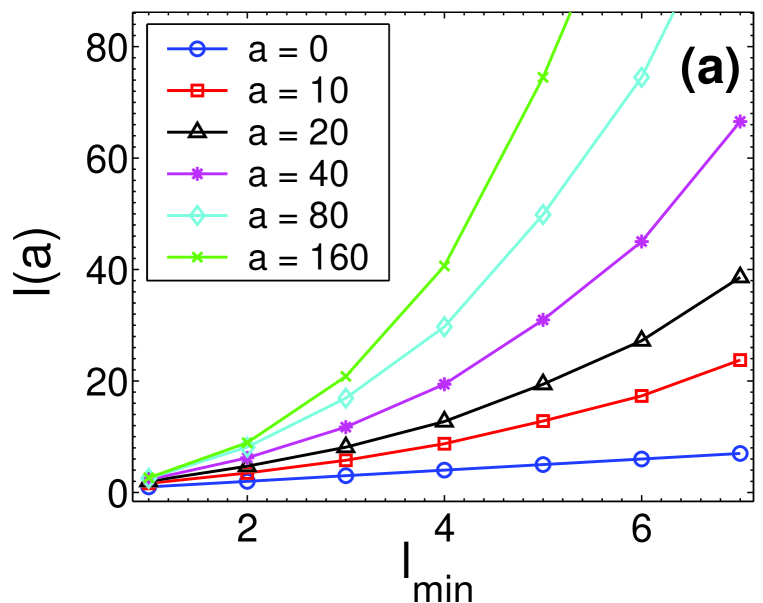
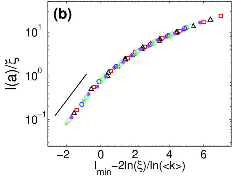
Figure 4: (Color online) Transition between different scaling regimes for the optimal path length $l(a)$ inside an ER graph with $N=128,000$ nodes and $\langle k\rangle=10$. (a) shows the unscaled and (b) shows the scaled length of the optimal path $l(a)$ averaged over all nodes with same value of $l_{min}$. Different symbols represent different values of the disorder strength $a$. Fig. (b) shows that for length scales $\ell(a)$ smaller than the “characteristic length”, $\xi=ap_{c}$, $l(a)$ grows exponentially relative to the shortest hopcount path $l_{min}$ (see solid line). This is consistent with $l(a)\sim N^{1/3}$ and $l_{min}\sim\log{N}$ inside the range of size $\xi=ap_{c}$. For length scales above $\xi$ both quantities scale as $\log{N}$.

We next present direct simulations supporting this argument. We calculate the optimal path length $l(a)$ inside a single network, for a given $a$, and find (Fig. 4) that it scales differently below and above the characteristic length $\xi=ap_{c}$. For each node in the graph we find $l_{min}$, which is the number of links (“hopcounts”) along the shortest path from the root to this node without regarding the weight of the link   . In Fig. 4 we plot the length of the optimal path $l(a)$, averaged over all nodes with the same value of $l_{min}$ for different values of $a$. The figure strongly suggests that $l(a)\sim\exp(l_{min})$ for length scales below the characteristic length $\xi=ap_{c}$, while for large length scales $l(a)\sim l_{min}$ . This is consistent with our hypothesis that below the characteristic length ($\xi=ap_{c}$) $l_{min}\sim\log{N}$ and $l(a)\sim N^{1/3}$, while $l_{min}\sim\log{N}$ and $l(a)\sim\log{N}$ above.

In order to better understand why the distributions of $l_{opt}$ depend on $Z$ according to Eq. (3), we suggest the following argument. The optimal path for $a\rightarrow\infty$, was shown to be proportional to $N^{1/3}$ for ER graphs and $N^{(\lambda-3)/(\lambda-1)}$ for SF graphs with $3<\lambda<4$ Braunstein et al. (2003). For finite $a$ the number of shortcuts, or number of blobs, is $Z=\frac{\ell_{\infty}}{\xi}=\frac{\ell_{\infty}}{ap_{c}}$. The deviation of the optimal path length for finite $a$ from the case of $a\rightarrow\infty$ is a function of the number of shortcuts. These results explain why the parameter $Z\equiv\frac{\ell_{\infty}}{ap_{c}}$ determines the functional form of the distribution function of the optimal paths.

IV Summary and Conclusions:

To summarize, we have shown that the optimal path length distribution in weighted random graphs has a universal scaling form according to Eq. (3). We explain this behavior and demonstrate the transition between polynomial to logarithmic behavior of the average optimal path in a single graph. Our results are consistent with results found for finite dimensional systems Porto et al. (1999); Z. Wu et al. (2005); Strelniker et al. (2005); Perlsman and Havlin (2005): In finite dimension the parameter controlling the transition is $\frac{L^{1/\nu}}{ap_{c}}$, where $L$ is the system length and $\nu$ is the correlation length critical exponent (for random graphs $\nu=1$ when calculated in the shortest path metric). This is because only the “red bonds” - bonds that if cut would disconnect the percolation cluster Coniglio (1982) - control the transition.

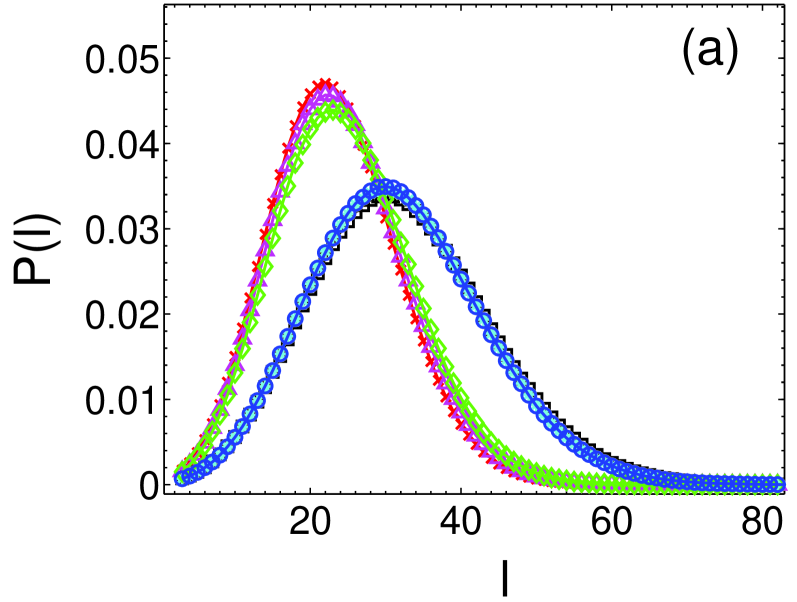
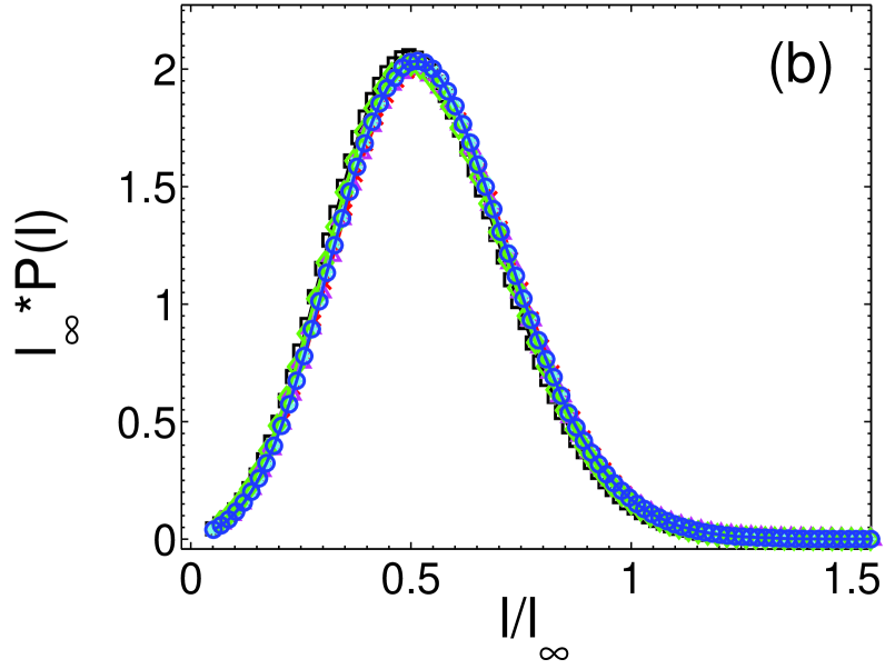
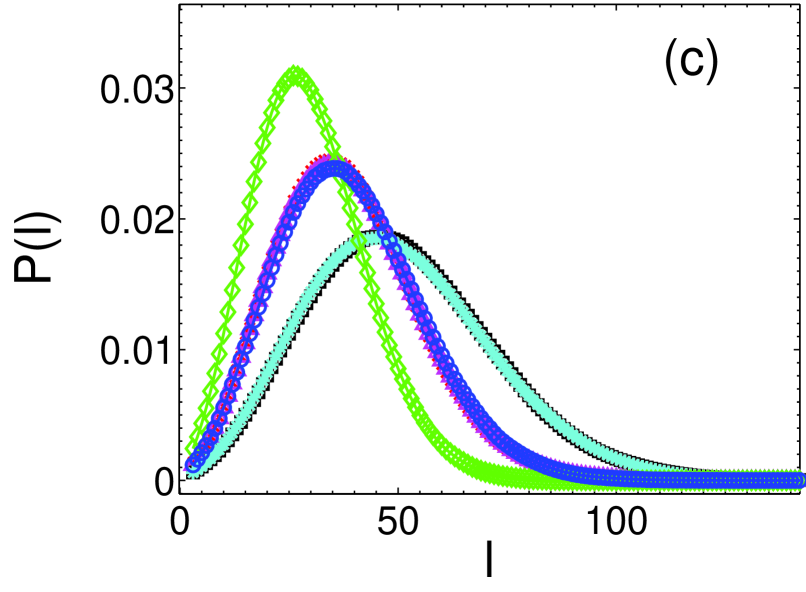
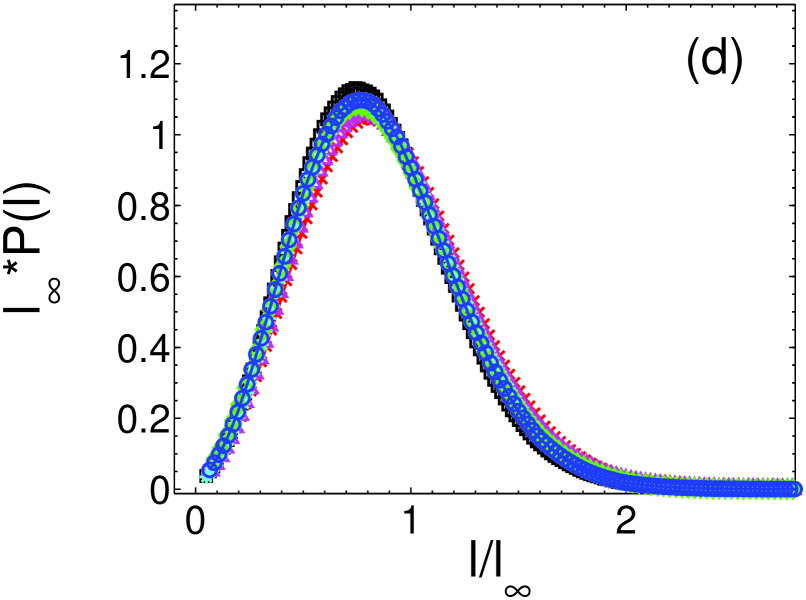
Figure 1: (Color online) Optimal path lengths distribution, $P(l)$, for ER networks with (a,b) $Z\equiv\frac{1}{p_{c}}\frac{\ell_{\infty}}{a}=10$ and (c,d) $Z=3$. (a) and (c) represent the unscaled distributions for $Z=10$ and $Z=3$ respectively, while (b) and (d) are the scaled distribution. Different symbols represent networks with different characteristics such as size $N$ (which determines $\ell_{\infty}\sim N^{1/3}$), average degree $\langle k\rangle$ (which determines $p_{c}=1/\langle k\rangle$), and disorder strength $a$ – see Table 1 for details. Results were averaged over $1500$ realizations.

$N$	$\langle k\rangle$	$\ell_{\infty}$	$p_{c}$	$a$	$Z=\frac{1}{p_{c}}\frac{\ell_{\infty}}{a}$	Symbol
4000	3	42.48	1/3	12.73	10	x
8000	3	60.59	1/3	18.16	10	$\Box$
4000	5	44.01	1/5	22.00	10	$\bigtriangleup$
8000	5	58.42	1/5	29.19	10	$\ast$
4000	8	45.99	1/8	36.78	10	$\diamond$
8000	8	58.25	1/8	46.60	10	$\circ$
4000	3	42.48	1/3	42.45	3	x
8000	3	60.59	1/3	60.55	3	$\Box$
4000	5	44.01	1/5	73.33	3	$\bigtriangleup$
8000	5	58.42	1/5	97.31	3	$\ast$
2000	8	34.94	1/8	93.15	3	$\diamond$
4000	8	45.99	1/8	122.62	3	$\circ$

Table 1: Different disordered ER graphs with same value of $Z=\frac{1}{p_{c}}\frac{\ell_{\infty}}{a}$. The symbols refer to Fig. 1.

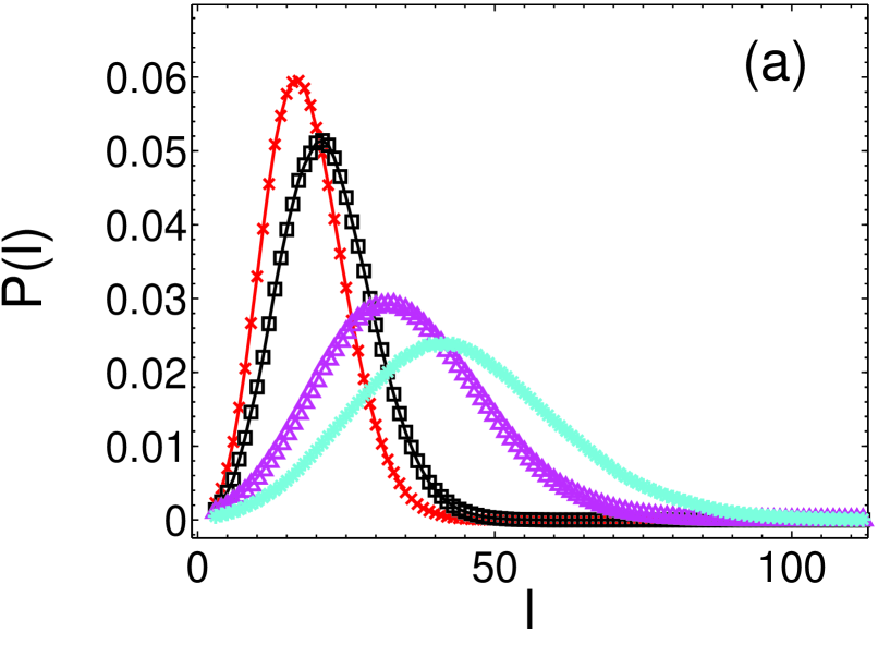
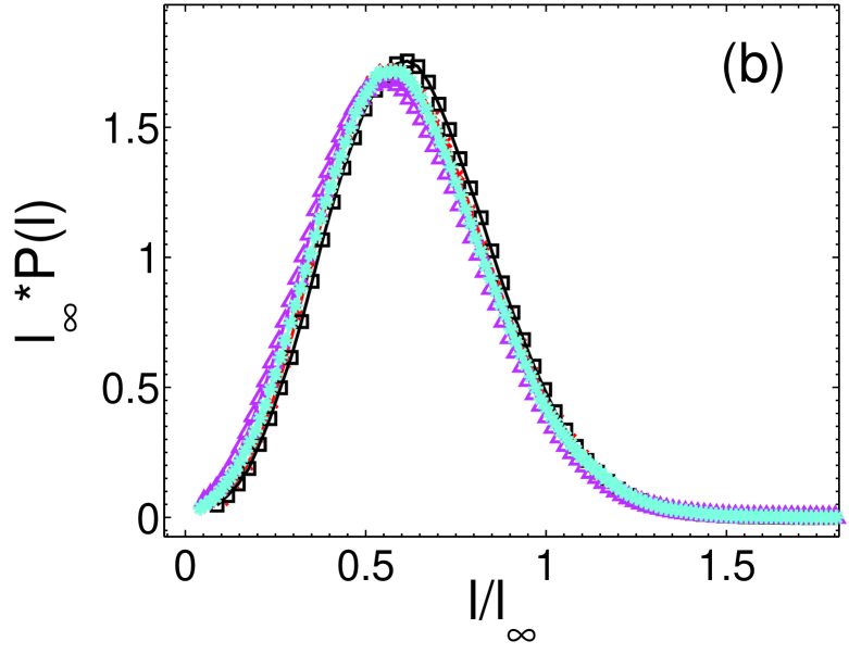
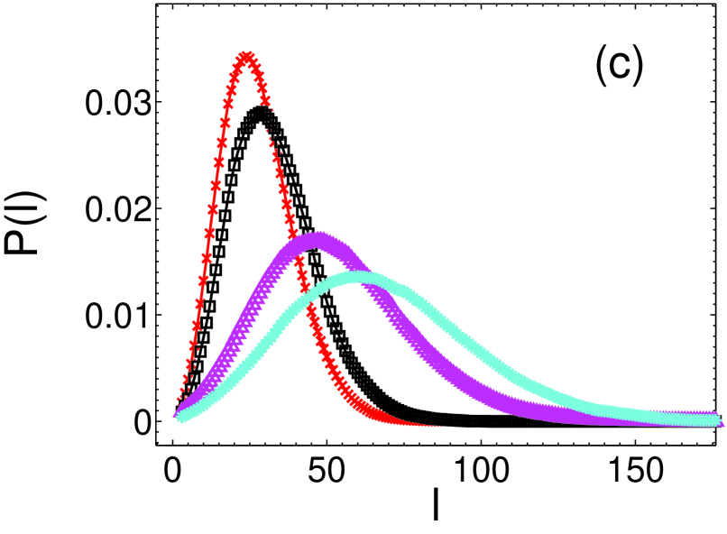
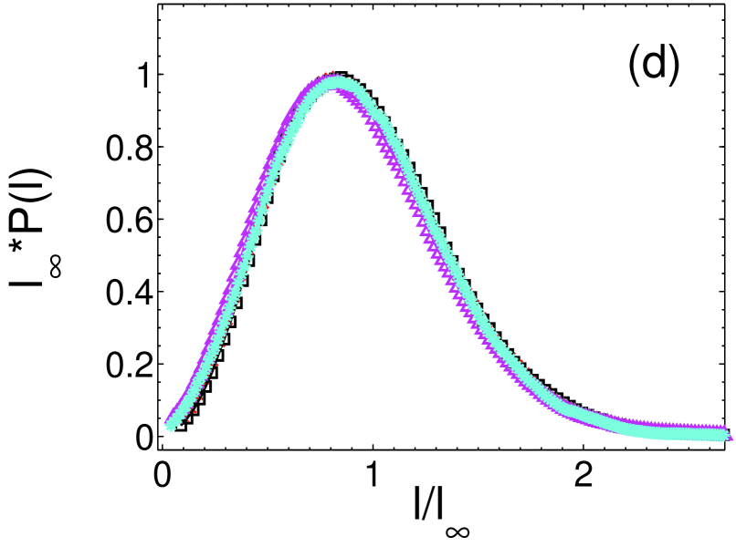
Figure 2: (Color online) Optimal path lengths distribution, $P(l)$, for SF networks with (a,b) $Z\equiv\frac{1}{p_{c}}\frac{\ell_{\infty}}{a}=10$ and (c,d) $Z=2$. (a) and (c) represent the unscaled distributions for $Z=10$ and $Z=2$ respectively, while (b) and (d) are the scaled distribution. Different symbols represent networks with different characteristics such as size $N$ (which determines $\ell_{\infty}\sim N^{\nu_{opt}}$), $\lambda$ and $m$ (which determine $p_{c}$), and disorder strength $a$ – see Table 2. Results were averaged over $250$ realizations.

$N$	$\lambda$	$m$	$\ell_{\infty}$	$p_{c}$	$a$	$Z=\frac{1}{p_{c}}\frac{\ell_{\infty}}{a}$	Symbol
4000	3.5	2	29.02	0.27	10.51	10	x
8000	3.5	2	34.13	0.26	12.88	10	$\Box$
4000	5	2	57.70	0.5	11.54	10	$\bigtriangleup$
8000	5	2	72.03	0.5	14.40	10	$\ast$
4000	3.5	2	29.02	0.27	52.56	2	x
8000	3.5	2	34.13	0.26	64.44	2	$\Box$
4000	5	2	57.70	0.5	57.70	2	$\bigtriangleup$
8000	5	2	72.03	0.5	72.03	2	$\ast$

Table 2: Different disordered SF graphs with same value of $Z=\frac{1}{p_{c}}\frac{\ell_{\infty}}{a}$. The percolation threshold was calculated according to: $p_{c}=\frac{\langle k\rangle}{\langle k(k-1)\rangle}$. The symbols refer to Fig. 2.

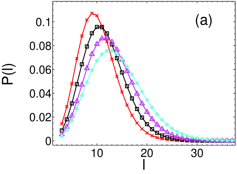
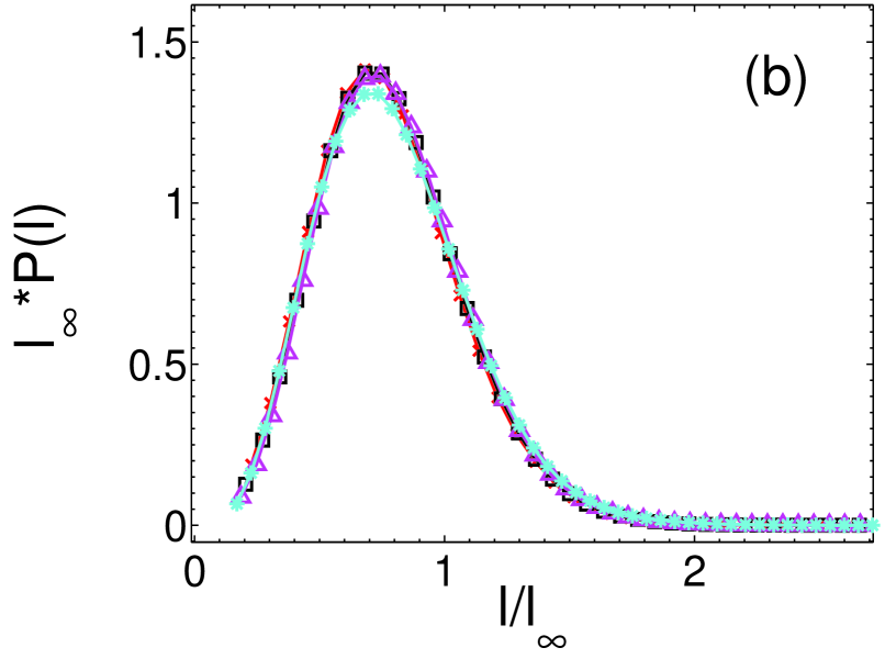
Figure 3: (Color online) Optimal path lenghts distribution function for SF graphs with $\lambda=2.5$, and with $Z\equiv\frac{1}{p_{c}}\frac{\ell_{\infty}}{a}=10$. (a) represents the unscaled distribution for $Z=10$ while (b) shows the scaled distribution. Different symbols represent graphs with different characteristics such as size $N$ (which determines $\ell_{\infty}\sim\log(N)$ and $p_{c}\sim N^{-1/3}$), and disorder strength $a$ – see Table 3. Results were averaged over $1500$ realizations.

$N$	$\lambda$	$m$	$\ell_{\infty}$	$p_{c}$	$a$	$Z=\frac{1}{p_{c}}\frac{\ell_{\infty}}{a}$	Symbol
2000	2.5	2	13.19	0.048	27.01	10	x
4000	2.5	2	14.66	0.037	38.70	10	$\Box$
8000	2.5	2	16.14	0.029	54.50	10	$\bigtriangleup$
16000	2.5	2	17.69	0.022	77.48	10	$\ast$

Table 3: Different disordered SF graphs with $\lambda=2.5$ and with same value of $Z=\frac{1}{p_{c}}\frac{\ell_{\infty}}{a}$. Notice that $p_{c}\sim N^{-1/3}\rightarrow 0$ for $N\rightarrow\infty$. The symbols refer to Fig. 3.

References

- Albert and Barabási (2002) R. Albert and A.-L. Barabási, Rev. of Mod. Phys. 74, 47 (2002).
- Dorogovtsev and Mendes (2003) S. N. Dorogovtsev and J. F. F. Mendes, Evolution of Networks - From Biological Nets to the Internet and WWW (Oxford University Press, 2003).
- Pastor-Satorras and Vespignani (2004) R. Pastor-Satorras and A. Vespignani, Evolution and Structure of the Internet : A Statistical Physics Approach (Cambridge University Press, 2004).
- Braunstein et al. (2003) L. A. Braunstein, S. V. Buldyrev, R. Cohen, S. Havlin, and H. E. Stanley, Phys. Rev. Lett. 91, 168701 (2003).
- Barrat et al. (2004) A. Barrat, M. Barthélemy, and A. Vespignani, Phys. Rev. Lett 92, 228701 (2004).
- Cieplak et al. (1994) M. Cieplak, A. Maritan, and J. R. Banavar, Phys. Rev. Lett. 72, 2320 (1994).
- Cieplak et al. (1996) M. Cieplak, A. Maritan, and J. R. Banavar, Phys. Rev. Lett. 76, 3754 (1996).
- Porto et al. (1997) M. Porto, S. Havlin, S. Schwarzer, and A. Bunde, Phys. Rev. Lett. 79, 4060 (1997).
- Sreenivasan et al. (2004) S. Sreenivasan, T. Kalisky, L. A. Braunstein, S. V. Buldyrev, S. Havlin, and H. E. Stanley, Phys. Rev. E 70, 046133 (2004).
- Braunstein et al. (2004) L. A. Braunstein, S. V. Buldyrev, S. Sreenivasan, R. Cohen, S. Havlin, and H. E. Stanley, in Lecture Notes in Physics: Proceedings of the 23rd LANL-CNLS Conference, ”Complex Networks”, Santa-Fe, New Mexico, May 12 - 16, 2003, edited by E. Ben-Naim, H. Frauenfelder, and Z. Toroczkai (Springer, Berlin, 2004).
- Cohen et al. (2000) R. Cohen, K. Erez, D. ben Avraham, and S. Havlin, Phys. Rev. Lett. 85, 4626 (2000).
- Cormen et al. (2001) T. H. Cormen, C. E. Leiserson, R. L. Rivest, and C. Stein, Introduction to Algorithms (MIT Press, 2001).
- Cohen and Havlin (2003) R. Cohen and S. Havlin, Phys. Rev. Lett. 90, 058701 (2003).
- Callaway et al. (2000) D. S. Callaway, M. E. J. Newman, S. H. Strogatz, and D. J. Watts, Phys. Rev. Lett. 85, 5468 (2000).
- Porto et al. (1999) M. Porto, N. Schwartz, S. Havlin, and A. Bunde, Phys. Rev. E 60, R2448 (1999).
- Z. Wu et al. (2005) E. L. Z. Wu, S. V. Buldyrev, L. A. Braunstein, S. Havlin, and H. E. Stanley, Phys. Rev. E (Rapid Communications) 71, 045101 (2005).
- Strelniker et al. (2005) Y. M. Strelniker, S. Havlin, R. Berkovits, and A. Frydman, Phys. Rev. E (In press) (2005).
- Perlsman and Havlin (2005) E. Perlsman and S. Havlin, Eur. Phys. J. B 43, 517 (2005).
- Coniglio (1982) A. Coniglio, J. Phys. A. 15, 3829 (1982).
- Bollobás (1980) B. Bollobás, Europ. J. Combinatorics 1, 311 (1980).
- Molloy and Reed (1998) M. Molloy and B. Reed, Combinatorics, Probability and Computing 7, 295 (1998).
- Xulvi-Brunet et al. (2003) R. Xulvi-Brunet, W. Pietsch, and I. M. Sokolov, Phys. Rev. E 68, 036119 (2003).
- Kalisky et al. (2004) T. Kalisky, R. Cohen, D. ben Avraham, and S. Havlin, in Lecture Notes in Physics: Proceedings of the 23rd LANL-CNLS Conference, ”Complex Networks”, Santa-Fe, 2003, edited by E. Ben-Naim, H. Frauenfelder, and Z. Toroczkai (Springer, Berlin, 2004).
- Aiello et al. (2000) W. Aiello, F. Chung, and L. Lu, in Annual ACM Symposium on Theory of Computing: Proceedings of the thirty-second annual ACM symposium on Theory of computing (Portland, Oregon, United States, 2000).