Interference pattern and visibility of a Mott insulator

Abstract

We analyze theoretically the experiment reported in [F. Gerbier et al, cond-mat/0503452], where the interference pattern produced by an expanding atomic cloud in the Mott insulator regime was observed. This interference pattern, indicative of short-range coherence in the system, could be traced back to the presence of a small amount of particle/hole pairs in the insulating phase for finite lattice depths. In this paper, we analyze the influence of these pairs on the interference pattern using a random phase approximation, and derive the corresponding visibility. We also account for the inhomogeneity inherent to atom traps in a local density approximation. The calculations reproduce the experimental observations, except for very large lattice depths. The deviation from the measurement in this range is attributed to the increasing importance of non-adiabatic effects.

The superfluid to Mott insulator (MI) transition undergone by an ultracold Bose gas in an optical lattice has attracted much attention in the recent years as a prototype for strongly correlated quantum phases Jaksch et al. (1998); Greiner et al. (2002a); Zwerger (2003); Stöferle et al. (2004). A key observable in these systems is the interference pattern observed after releasing the gas from the lattice and letting it expand for a certain time of flight. Monitoring the evolution of this interference pattern not only reveals the superfluid-to-MI transition Greiner et al. (2002a); Stöferle et al. (2004), but also allows for example the detection of number-squeezed states in the lattice Orzel et al. (2001); Hadzibabic et al. (2004), or the observation of collapse and revivals of coherence due to atomic interactions Greiner et al. (2002b). Because of its experimental importance, a quantitative understanding of this interference signal is crucial to characterize quantum phases of bosons in optical lattices.

Although no interference pattern is expected for a uniform array of Fock states (what we call a “perfect” Mott Insulator) , a finite visibility is nevertheless observed in experiments above the insulator transition Greiner et al. (2002a); Stöferle et al. (2004); Gerbier et al. (2005), in agreement with numerical calculations Kashurnikov et al. (2002); Roth and Burnett (2003). We have studied this phenomenon experimentally, and shown that despite its insulating nature that forbids long-range coherence, a MI still exhibits short-range coherence at the scale of a few lattice sites Gerbier et al. (2005). This can be attributed to the structure of the ground state for finite lattice depths, which consists of a small admixture of particle/hole pairs on top of a perfect MI. A qualitative model based on a lowest-order calculation of the ground state wavefunction was also presented in our previous work, which reproduced the main trend and order of magnitude of the observed visibility.

In the present paper, we would like to present a more precise calculation that includes higher order corrections (see also Yu (2005)). We describe a MI state at zero temperature using the Random Phase Approximation (RPA), already introduced in Refs. van Oosten et al. (2001); Dickerscheid et al. (2003); Gangardt et al. (2004); Sengupta and Dupuis (2005); van Oosten et al. (2005). Instead of the path integral approach used by these authors, we obtain here the RPA Green’s function using a different method inspired by Hubbard’s original treatment of the fermionic model Hubbard (1963, 1964). Taking the experimental geometry and the inhomogeneous particle distribution into account, we find good agreement with our experimental data, which provides further support for the physical picture presented above.

The paper is organized as follows. In section I, we recall the description of ultracold atoms in an optical lattice by the Bose-Hubbard model, and discuss the inhomogeneous shell structure that develops in an external confining potential. Section II presents the calculation of the interference pattern observed after free expansion of the atom cloud and its link with the quasi-momentum distribution. The main results are presented in sections III and IV, where we respectively present the calculation of the interference pattern in the uniform case using the RPA, and extend it to the inhomogeneous case to compare to the experimental data of Gerbier et al. (2005). Details of the calculation are described in the appendix.

I Bose-Hubbard hamiltonian

In this section, we briefly recall the theoretical description of an ultracold atomic gas trapped in an optical lattice. The optical lattice potential, which results from the superposition of three orthogonal and independent pairs of counterpropagating laser beams, can be written as

$$V_{\rm OL}({\bf r})=V_{0}\left(\sin^{2}(k_{\rm L}x)+\sin^{2}(k_{\rm L}y)+\sin^{2}(k_{\rm L}z)\right),$$ (1)

Here $V_{0}$ is the lattice depth, $k_{\rm L}=2\pi/\lambda_{\rm L}$ is the laser wavevector, $\lambda_{\rm L}$ is the laser wavelength and $m$ is the atomic mass. As usual, we measure $V_{0}$ in units of the single-photon recoil energy $E_{\rm R}=h^{2}/2m\lambda_{\rm L}^{2}$. The lattice potential has a simple cubic periodicity in three dimensions, with a lattice spacing $d=\lambda_{\rm L}/2\approx 425~{}$nm in our case. As shown in Jaksch et al. (1998), the behavior of the atomic system in such a potential can be described by the Bose-Hubbard model, defined by the hamiltonian

$$\mathcal{H} = -t\sum_{\langle i,j\rangle}\hat{a}_{i}^{\dagger}\hat{a}_{j}+\sum_{i}\frac{U}{2}\hat{n}_{i}\left(\hat{n}_{i}-1\right).$$ (2)

Here the operator $\hat{a}_{i}^{\dagger}$ creates an atom at site $i$, $\hat{n}_{i}=\hat{a}_{i}^{\dagger}\hat{a}_{i}$ is the on-site number operator, and the notation $\langle i,j\rangle$ restricts the sum to nearest neighbors only. The relative strength between the tunneling matrix element $t$ and the on-site interaction energy $U$ is controlled by the depth $V_{0}$ of the periodic potential which confines the atoms . The phase diagram of this hamiltonian is well known: The system is in a MI state within characteristic lobes in a $t/U$ versus chemical potential $\mu$ phase diagram, and in a superfluid state outside of these lobes Fisher et al. (1989).

In the experiments, an additional potential $V_{\rm ext}({\bf r})$ is superimposed to the lattice potential, leading to a spatially varying chemical potential across the cloud. This favors the formation of a “wedding cake” structure of alternating MI and superfluid shells, which reflects the phase diagram of the Bose-Hubbard model Fisher et al. (1989); Jaksch et al. (1998); Kashurnikov et al. (2002); Batrouni et al. (2002). The external potential is due to a combination of a magnetic potential in which the condensate is initially formed and of an optical potential due to the Gaussian shape of the lattice beams. To a good approximation, it can be considered as a harmonic potential with trapping frequency

$$\Omega=\sqrt{\omega_{\rm m}^{2}+\frac{8V_{0}}{mw^{2}}},$$ (3)

where $\omega_{\rm m}$ is the frequency of the magnetic trap, assumed isotropic, and where $w$ is the waist ($1/e^{2}$ radius of the intensity profile) of the lattice beams, assumed identical for all axes. For large lattice depths, the confinement is mainly due to the optical part.

In the current experiments, this external potential varies slowly across the lattice. In this limit, the shell structure can be calculated in a local density approximation, which assumes a known relation $n_{\rm h}[\mu]$ between the density $n$ and the chemical potential $\mu$ for the homogeneous system. Then, the coarse-grained density for the inhomogeneous system is calculated as $n({\bf r})=n_{\rm h}[\mu-V_{\rm ext}({\bf r})]$. The chemical potential is fixed by the relation $N=\int d^{(3)}{\bf r}~{}n({\bf r})$. For a fixed lattice depth and atom number, we calculate numerically the relation $n_{\rm h}[\mu]$ using mean-field theory at zero temperature, i.e. in the mean-field ground state Sheshadri et al. (1993); van Oosten et al. (2001). We then repeat the steps outlined above, varying the chemical potential until the target atom number is obtained within 0.1 %. For all calculations, the values $\omega_{\rm m}=2\pi\times 15~{}$Hz and $w=130~{}\mu$m are used, which match our experimental parameters. We show in Fig. 1 an example of such a calculation for a lattice depth of $V_{0}=18~{}E_{\rm R}$ and $N=2.2\times 10^{5}$ atoms.

The presence of the external potential significantly affects the atom distribution in the lattice, which is determined by the competition between interaction and potential energy. On the one hand, expanding the cloud minimizes the density and the interaction energy, and on the other, contracting it minimizes the potential energy, as in conventional harmonic traps Dalfovo et al. (1999); Gerbier et al. (2004). The latter is favored at low atom numbers, where only a $n_{0}=1$ shell forms. When more atoms are added, the radius of the unity filled MI region increases until a critical atom number, which we estimate to be $7\times 10^{4}$ atoms for our parameters, is reached. Above this critical atom number, a higher density core appears near the trap center. A MI with $2$ atoms per site is then obtained near the trap center if the lattice depth is above the critical value $V_{0}\approx 14.7~{}E_{\rm R}$. This value has been calculated using the boundary derived in van Oosten et al. (2001),

$$\left(\frac{U}{zt}\right)_{n_{0}}=2n_{0}+1+2\sqrt{n_{0}(n_{0}+1)},$$ (4)

where $z=6$ is the number of nearest neighbors in 3 dimensions. In the specific example shown in Fig. 1, we have chosen $V_{0}=18~{}E_{\rm R}$ and $N=2.2\times 10^{5}$ atoms, so that both $n_{0}=1$ and $n_{0}=2$ MI are present. Similarly, we calculate for our experimental parameters that an $n_{0}=3$ shell is also present for atom numbers larger than $2.7\times 10^{5}$, and lattice depths larger than $16~{}E_{\rm R}$.

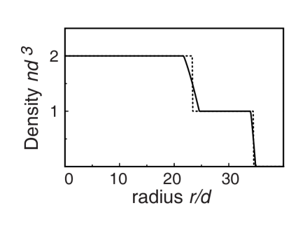
Figure 1: Calculated density profile for a lattice depth $V_{0}=18~{}E_{\rm R}$ and $N=2.2\times 10^{5}$ atoms. Here $d$ is the lattice spacing. The upper solid line indicates the numerical calculation of the total density, and the dotted line is the $U\rightarrow\infty$ extrapolation (see section IV).

II Interference pattern

We now turn to the description of the interference pattern observed after release of the atom cloud from the optical lattice and a period of free expansion. From an absorption image of such a pattern, the phase coherence of the atomic sample can be directly probed. The density distribution of the expanding cloud after a time of flight $t_{\rm f}$ can be calculated as Zwerger (2003); Pedri et al. (2001); Kashurnikov et al. (2002)

$$n({\bf r})=\left(\frac{m}{\hbar t_{\rm f}}\right)^{3}\left|\tilde{w}\left(\frac{m{\bf r}}{\hbar t_{\rm f}}\right)\right|^{2}\mathcal{S}\left({\bf k}=\frac{m{\bf r}}{\hbar t_{\rm f}}\right),$$ (5)

which mirrors the momentum distribution of the original cloud. Momentum space and real space in the image plane are related by the scaling factor $\hbar t_{\rm f}/m$ - independent of the lattice parameters. The envelope $\left|\tilde{w}\right|^{2}$ is the Fourier transform of the Wannier function in the lowest Bloch band. When each potential well is approximated as an harmonic potential, the Wannier function is the corresponding gaussian ground state wavefunction. The envelope function in Eq. (5) then reads

$$\left|\tilde{w}\left(\frac{m{\bf r}}{\hbar t_{\rm f}}\right)\right|^{2}\approx\frac{1}{\pi^{3/2}w_{t_{\rm f}}}\exp{\left(-\frac{{\bf r}^{2}}{w_{t_{\rm f}}^{2}}\right)},$$ (6)

where $w_{t_{\rm f}}=\hbar t_{\rm f}/mw_{0}$, and where $w_{0}$ is the size of the on-site Wannier function. Finally, we have defined the quantity

$$\mathcal{S}({\bf k})=\sum_{i,j}e^{i{\bf k}\cdot({\bf r}_{i}-{\bf r}_{j})}\langle\hat{a}_{i}^{\dagger}\hat{a}_{j}\rangle.$$ (7)

When ${\bf k}$ is restricted to the first Brillouin zone, $\mathcal{S}({\bf k})$ is nothing else than the quasi-momentum distribution. Information about the many-body system is contained in this quantity, which is periodic with the periodicity of the reciprocal lattice $2\pi/d$. Thus, to predict the interference pattern and compare to the experiments, our goal is to calculate $\mathcal{S}({\bf k})$ for a given lattice depth and density.

III Quasi-momentum distribution in the homogeneous Mott insulator

For simplicity, we consider first the case of uniform filling in the lattice, i.e. an integer number $n_{0}$ of atoms per site, and we assume the system to be at zero temperature and in the insulating phase. In the limit of zero tunneling, the ground state wavefunction is a perfect MI, i.e. a product of number states at each site, and its Green function $G_{0}$ can be calculated exactly (see appendix). The lowest-lying excited states of the system are “particle” and “hole” states, where a supplementary particle is added (respectively removed) at one lattice site. Creating these excitations costs a finite interaction energy, respectively $E^{(+)}=Un_{0}$ and $E^{(-)}=U(n_{0}-1)$ Fisher et al. (1989).

To calculate the quasi-momentum distribution for a finite tunneling $t$, many-body techniques can be applied to obtain the single-particle Green function, $G({\bf k},\omega)$. Using a path integral approach, several authors van Oosten et al. (2001); Dickerscheid et al. (2003); Gangardt et al. (2004); Sengupta and Dupuis (2005); van Oosten et al. (2005) have been able to calculate the Green function of the Mott insulator within the RPA,

$$\frac{1}{\hbar}G({\bf k},\omega)=\frac{Z_{\bf k}}{\hbar\omega+\mu-E_{\bf k}^{(+)}}+\frac{1-Z_{\bf k}}{\hbar\omega+\mu-E_{\bf k}^{(-)}}.$$ (8)

The poles $E_{\bf k}^{(\pm)}$ of the Green function are the quasi-particle energies van Oosten et al. (2001)

$$E_{\bf k}^{(\pm)}=\frac{t_{\bf k}}{2}+U(n_{0}-\frac{1}{2})\pm\frac{1}{2}D_{\bf k}[n_{0}],$$ (9)

In Eq. (9), $t_{\bf k}=-2t\sum_{\nu=x,y,z}\cos(k_{\nu}d)$ is the dispersion relation for a free particle in the tight-binding limit, and $D_{\bf k}[n_{0}]=\sqrt{t_{\bf k}^{2}+4t_{\bf k}U(n_{0}+\frac{1}{2})+U^{2}}$. The particle weight is $Z_{\bf k}=\left(E_{{\bf k}}^{(+)}+U\right)/D_{\bf k}[n_{0}]$. In the Appendix, we present an alternative derivation of (8) based on the equation of motion method, which follows closely Hubbard’s method Hubbard (1963, 1964). Here we will simply comment on the physical picture behind this approach. The RPA considers that the particle/hole nature of the low-lying excitations is not significantly changed by introducing a finite tunneling (in technical terms, the self energy remains approximately the same as in the $t\rightarrow 0$ limit). The first effect of tunneling is to introduce a finite amount of particle/hole components in the the many-body ground state wavefunction. In the form given in Gerbier et al. (2005), corresponding to a first order calculation, a particle/hole pair necessarily occupies two neighboring lattice sites due to the particular form of the tunneling hamiltonian. Through higher-order tunneling processes captured by the Green function (8), the particle and the hole forming the pair can tunnel independently. As a result, the pair acquires a mobility through the lattice, and may even “stretch” over a few lattice sites. This mobility acquired by particle/hole pairs is reflected in the modified dispersion relation (9), which explicitly includes the band structure. Note finally that higher order excitations, corresponding to occupation numbers $n_{0}\pm 2,n_{0}\pm 3$, … are neglected. At zero temperature, such excitations become important only very close to the superfluid transition where the MI is destroyed.

The quasi-momentum distribution can be directly deduced using the general relation $\mathcal{S}({\bf k})=-i\lim_{\delta t\rightarrow 0^{+}}\int\frac{d\omega}{2\pi}~{}G({\bf k},\omega)e^{-i\omega\delta t}$. Using (8), one has Sengupta and Dupuis (2005)

$$\mathcal{S}({\bf k})=n_{0}\left(\frac{\frac{t_{\bf k}}{2}+U(n_{0}+\frac{1}{2})}{\sqrt{t_{\bf k}^{2}+4t_{\bf k}U(n_{0}+\frac{1}{2})+U^{2}}}-\frac{1}{2}\right).$$ (10)

To first order in $t/U$, this reduces to

$$\mathcal{S}({\bf k})\approx n_{0}-2n_{0}(n_{0}+1)t_{\bf k}/U,$$ (11)

also obtained in Gerbier et al. (2005) by calculating the many-body wave function perturbatively. We find that the two predictions rapidly converge. For example, they differ by less than 10 % for $U/zt>6.6,11.6$ and $16.9$ for $n_{0}=1,2$ and $3$, respectively. These values have to be compared to the respective critical values for MI formation, $U/zt=5.83,9.89,13.93$. This indicates that the coherence beyond nearest neighbors is rather rapidly lost as one goes further into the MI phase. However, the visibility itself remains finite in a substantial range of $U/zt$, implying a persistent short-range coherence.

IV Comparison with the experiments

To compare with the experiments reported in Gerbier et al. (2005), several features have to be taken into account. First, only the column density $n$ is accessible experimentally, i.e. the density integrated along the probe line-of-sight (which we take here parallel to the $z$ axis). Second, the visibility is experimentally deduced from two points according to

$$\mathcal{V}_{\rm exp}=\frac{n_{\rm max}-n_{\rm min}}{n_{\rm max}+n_{\rm min}}.$$ (12)

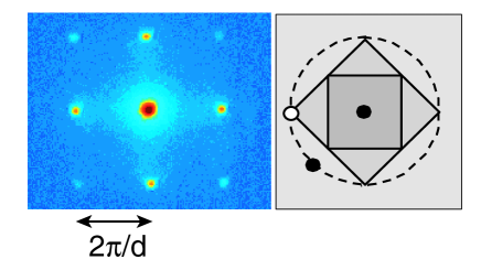
Figure 2: Measurement of visibility. The interference pattern shown in the left graph corresponds to a lattice depth of $8~{}E_{\rm R}$, in the superfluid regime. The right graph indicates the geometry of the reciprocal lattice. Gray areas are the first and second Brillouin zones (projected in the image plane), and the white dot indicate the position of the maxima of the interference pattern. Along the circle, the Wannier function envelope takes the same value, and we measure the interference “minimum” at the intersection of this circle and of the diagonal of the lattice square lattice, indicated by the black dot.

To eliminate the Wannier envelope, $n_{\rm max}$ and $n_{\rm min}$ are measured from two points at the same distance from the cloud center (see Fig. 2), so that the envelope automatically cancels out. For example, $n_{\rm max}$ is found at point $(2\pi/d,0)$ and $n_{\rm min}$ at $(2\pi/\sqrt{2}d,2\pi/\sqrt{2}d)$. This reduces the visibility compared to the usual definition. In the theoretical calculation it is straightforward to account for these two effects.

The third effect, the shell structure of the MI, is handled here in an approximate way. In the numerical calculations, the shell distribution always includes small regions with non-integer filling, which the theory above cannot handle. However, these domains are small, and have a strongly depleted superfluid component, so that we do not expect them to have a large effect on the visibility. Therefore, we approximate the density distribution by a “ziggurat”-like profile, where only MI shells are present. The actual extension of each shell is calculated as if $t$ were zero, taking the external potential into account DeMarco et al. (2005). In Fig. 1, we compare the profile in this approximation (dotted line) with the numerically calculated one (solid line). For large lattice depths, both agree reasonably. Note that the density profile still depends weakly on the lattice depth through the external confinement [see Eq. (3)].

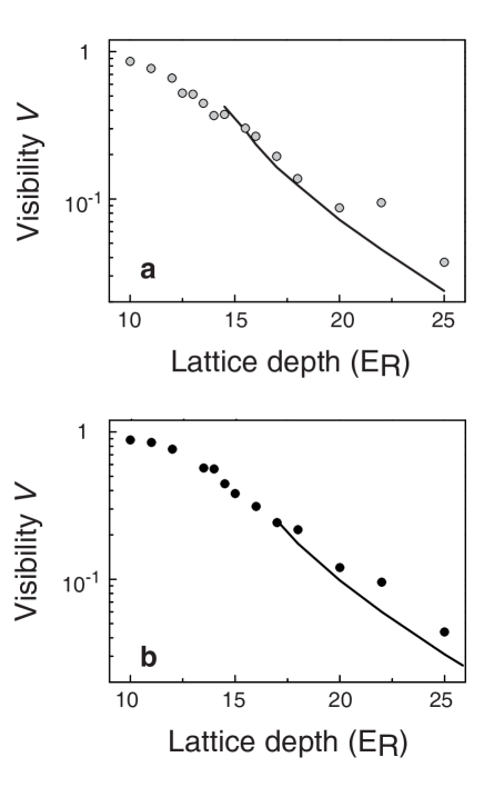
Figure 3: Comparison between the measured and the calculated visibility. The upper and lower graphs correspond to atom numbers $N=2.2\times 10^{5}$ and $N=5.6\times 10^{5}$, respectively. The dotted and dashed lines indicate the calculated visibility for homogeneous MI with filling factor $n_{0}=1,2$. The solid lines are calculations including the inhomogeneous shell distribution. Typical standard deviations for the experimental data are 1 % or below. Our calculation of the equilibrium distribution at zero temperature indicate that in case a, only MI regions with $n_{0}=1$ and $n_{0}=2$ atoms per site form, whereas in case b, a core with $n_{0}=3$ is also present.

The momentum distribution deduced from Eqs. (5,10) is averaged over the distribution of atoms to compare with the experimental data (see Gerbier et al. (2005) for details on the experiment). The results are plotted versus lattice depth in Fig. 3, for two different atom numbers in the lattice. For the lowest atom number $N=2.2\times 10^{5}$, we calculate that only $n_{0}=1$ and $n_{0}=2$ shells are present. For the largest $N=5.6\times 10^{5}$, a core with $n_{0}=3$ atoms per site is also present. Note that in the latter case, the actual density distribution might deviate more from the calculated one, due to three-body losses in the $n_{0}=3$ region. We find that the calculation agrees with the measured visibility within 20 % for $V_{0}\leq 22~{}E_{\rm R}$. The theory curves terminate when the MI shell with highest filling disappears, as it is replaced by a large superfluid core not described by our theory. Note that the calculation does not include any free parameter.

However, we consistently find that the calculated value lies below the measured visibility for large lattice depths $V_{0}\leq 22~{}E_{\rm R}$. Moreover, the deviation increases with increasing lattice depths, which shows that the superfluid shells play little role in determining the visibility for such large lattice depths, as assumed in our calculation. In Fig. 4, the fractional deviation of the calculated visibility from the measured one is plotted versus lattice depth for four data sets. Remarkably, although the atom numbers are rather different from one data set to another we find a common trend in the data. On the other hand, this observation also suggests that a breakdown of adiabaticity occurs for the particular ramp used in the experiments to increase the laser intensity to its final value, a point already identified in Gerbier et al. (2005). We conclude that, perhaps surprisingly, the visibility in the MI may be a sensitive probe of the many-body dynamics of the superfluid-to-insulator transition.

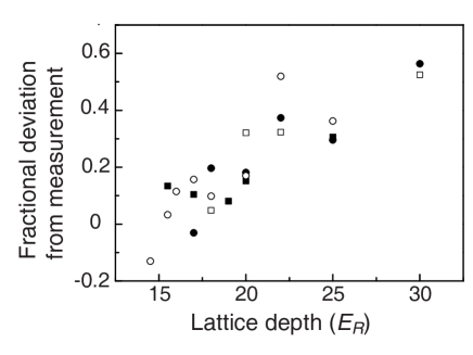
Figure 4: Fractional deviation of the calculated visibility from the measurements. Symbols denote different data sets with different atom numbers and densities ($\square$: $N=2.2\times 10^{5}$, $\blacksquare$: $N=3.6\times 10^{5}$, $\medcirc$: $N=4.3\times 10^{5}$, $\medbullet$: $N=5.9\times 10^{5}$).

V Conclusion

In conclusion, we have derived in this paper a theoretical expression for the interference pattern of a Mott insulator after release from the optical lattice and a time of flight. Our calculations take deviations from perfect filling due to a finite tunneling into account, and use a simplified but realistic model of the shell structure of the MI. Good agreement with our experimental data reported in Gerbier et al. (2005) is found, at least for moderate lattice depths. For very large lattice depths, an increasing deviation points to non-adiabatic effects in the conversion from a condensate to an insulating state, which could in principle be studied by the method presented here. Nevertheless, in view that no free parameter is included in the theory, we conclude that the momentum distribution (10) describes the system well. This supports the physical picture of the system as a (dilute) gas of partice/hole pairs, mobile through the lattice, on top of a regularly filled Mott insulator. Furthermore, the validity of the RPA to describe their behavior is qualitatively verified.

Our calculation neglects entirely the superfluid component, which is correct only for large lattice depths where the system is almost completely insulating. Recently, several authors Garcia-Ripoll et al. (2004); Schroll et al. (2004); Sengupta and Dupuis (2005) have proposed to modify the standard mean-field description Fisher et al. (1989); Sheshadri et al. (1993) to better account for long- and short-range coherence. It would be interesting to compare the predictions of those approaches with our data for lower lattice depths, where the system is expected to be a strongly depleted superfluid, and therefore amenable neither to a Bogoliubov-like description nor to a strongly interacting one as provided in this paper. Also, an investigation of finite temperature effects Dickerscheid et al. (2003) would be useful. In particular, an interesting question is to know whether the visibility measurements presented here could be used for thermometry in the lattice.

We would like to thank Dries van Oosten, Paolo Pedri and Luis Santos for useful discussions. Our work is supported by the Deutsche Forschungsgemeinschaft (SPP1116), the European Union under a Marie-Curie Excellence Grant and AFOSR. FG acknowledges support from a Marie-Curie Fellowship of the European Union.

Appendix A Green function of the homogeneous Mott insulator in the Random Phase approximation

In this Appendix, we present a derivation of Eq. (8) using the equation of motion approach. The single-particle Green function is defined at zero temperature as

$$G_{ij}(t) = -i\langle\mathcal{T}\hat{a}_{i}(0)\hat{a}_{j}^{\dagger}(t)\rangle$$

$$= -i\theta(t)\langle\hat{a}_{i}(0)\hat{a}_{j}^{\dagger}(t)\rangle$$

$$-i\theta(-t)\langle\hat{a}_{j}^{\dagger}(t)\hat{a}_{i}(0)\rangle,$$

where $\mathcal{T}$ is the time-ordering operator and $\theta$ is the Heaviside step function. Since we consider a time-independent and homogeneous system, we take a Fourier transformation of this equation with respect to space and time (denoted by the symbol $\mathcal{F}$), and define

$$G({\bf k},\omega) = \mathcal{F}\left[G_{ij}(t)\right]$$ (14)

In the frequency-momentum representation, the Heisenberg equation of motion $i\hbar\frac{\partial}{\partial t}G_{ij}(t)=\left[H,G_{ij}(t)\right]$ takes the form

$$(\hbar\omega+\mu)G({\bf k},\omega) = 1+t_{\bf k}G({\bf k},\omega)$$ (15)

$$-i\mathcal{F}\left[\langle\mathcal{T}n_{i}\hat{a}_{i}(0)\hat{a}_{j}^{\dagger}(t)\rangle\right].$$

The last term on the right hand side of (15) is usually rewritten as $\Sigma({\bf k},\omega)G({\bf k},\omega)$, where $\Sigma$ is the self-energy. This gives the expression

$$G({\bf k},\omega) = \frac{1}{\hbar\omega+\mu-t_{\bf k}-\Sigma({\bf k},\omega)}.$$ (16)

Let us first assume that no tunneling is present ($t=0$). In this case, the Green function can be obtained exactly from its definition (A) and the ground state wave function $|\Psi\rangle=\prod_{i}|n_{0}\rangle_{i}$, where each site is in the Fock state $|n_{0}\rangle$. The result $G_{0}(\omega)$ is independent of momentum, and reads

$$G_{0}(\omega)=\frac{n_{0}+1}{\hbar\omega+\mu-Un_{0}}-\frac{n_{0}}{\hbar\omega+\mu-U(n_{0}-1)}.$$ (17)

In this self-interacting limit, we can rewrite Eq. (17) as $G_{0}(\omega)^{-1}=\hbar\omega+\mu-\Sigma_{0}(\omega)$, with the self energy van Oosten et al. (2005)

$$\Sigma_{0}(\omega)=2Un_{0}-\frac{U^{2}n_{0}(n_{0}+1)}{\hbar\omega+\mu+U}.$$ (18)

This expression is exact in the $t\rightarrow 0$ limit, and coincides with the one found in van Oosten et al. (2005). The first term is simply the Hartree-Fock energy per particle for uncondensed atoms (hence the factor of $2$), whereas the second term - which has the same order of magnitude at low energy - accounts for the correlations between particle that drive the system into the perfectly ordered ground state.

If we now restore a finite tunneling, but still consider a system in the insulating phase, a reasonable approximation is to assume that the self energy is not changed with respect to the strongly interacting limit. We comment on this approximation in the test. Making this approximation yields

$$G({\bf k},\omega) \approx \frac{1}{\hbar\omega+\mu-t_{\bf k}-\Sigma_{0}(\omega)}$$ (19)

$$= \frac{G_{0}(\omega)}{1-t({\bf k})G_{0}(\omega)},$$

which has a typical RPA form. Using the explicit result for $G_{0}$, we obtain after some algebra Eq. (8) in the text, which explicitly displays particle and hole components.

References

- Jaksch et al. (1998) D. Jaksch, C. Bruder, J. I. Cirac, C. W. Gardiner, and P. Zoller, Phys. Rev. Lett. 81, 3108 (1998).
- Greiner et al. (2002a) M. Greiner, O. Mandel, T. Esslinger, T. W. Hänsch, and I. Bloch, Nature 415, 39 (2002a).
- Zwerger (2003) W. Zwerger, J. Opt. B: Quantum Semiclass. Opt. 5, S9 (2003).
- Stöferle et al. (2004) T. Stöferle, H. Moritz, C. Schori, M. Köhl, and T. Esslinger, Phys. Rev. Lett. 92, 130403 (2004).
- Orzel et al. (2001) C. Orzel, A. K. Tuchman, M. L. Fenselau, M. Yasuda, and M. K. Kasevich, Science 291, 2386 (2001).
- Hadzibabic et al. (2004) Z. Hadzibabic, S. Stock, B. Battelier, V. Bretin, and J. Dalibard, Phys. Rev. Lett. 93, 180403 (2004).
- Greiner et al. (2002b) M. Greiner, O. Mandel, T. W. Hänsch, and I. Bloch, Nature 419, 51 (2002b).
- Gerbier et al. (2005) F. Gerbier, A. Widera, S. Fölling, O. Mandel, T. Gericke, and I. Bloch, cond-mat/0503452 (2005).
- Kashurnikov et al. (2002) V. A. Kashurnikov, N. V. Prokof’ev, and B. V. Svistunov, Phys. Rev. A 66, 031601(R) (2002).
- Roth and Burnett (2003) R. Roth and K. Burnett, Phys. Rev. A 67, 031602(R) (2003).
- Yu (2005) Y. Yu, cond-mat/0505181 (2005).
- van Oosten et al. (2001) D. van Oosten, P. van der Straten, and H. T. C. Stoof, Phys. Rev. A 63, 053601 (2001).
- Dickerscheid et al. (2003) D. B. M. Dickerscheid, D. van Oosten, P. J. H. Denteneer, and H. T. C. Stoof, Phys. Rev. A 68, 043623 (2003).
- Gangardt et al. (2004) D. M. Gangardt, P. Pedri, L. Santos, and G. V. Shlyapnikov, cond-mat/0408437 (2004).
- Sengupta and Dupuis (2005) K. Sengupta and N. Dupuis, Phys. Rev. A 71, 033629 (2005).
- van Oosten et al. (2005) D. van Oosten, D. B. M. Dickerscheid, B. Farid, P. van der Straten, and H. T. C. Stoof, Phys. Rev. A 71, 021601(R) (2005).
- Hubbard (1963) J. Hubbard, Proc. Roy. Soc. A276, 238 (1963).
- Hubbard (1964) J. Hubbard, Proc. Roy. Soc. A281, 401 (1964).
- Fisher et al. (1989) M. P. A. Fisher, P. B. Weichman, G. Grinstein, and D. S. Fisher, Phys. Rev. B 40, 546 (1989).
- Batrouni et al. (2002) G. G. Batrouni, V. Rousseau, R. T. Scalettar, M. Rigol, A. Muramatsu, P. J. H. Denteneer, and M. Troyer, Phys. Rev. Lett. 89, 117203 (2002).
- Sheshadri et al. (1993) K. Sheshadri, H. R. Krishnamurthy, R. Pandit, and T. V. Ramakrishnan, Euro. Phys. Lett. 22, 257 (1993).
- Dalfovo et al. (1999) F. Dalfovo, S. Giorgini, L. P. Pitaevskii, and S. Stringari, Rev. Mod. Phys. 71, 463 (1999).
- Gerbier et al. (2004) F. Gerbier, J. H. Thywissen, S. Richard, M. Hugbart, P. Bouyer, and A. Aspect, Phys. Rev. A 70, 013607 (2004).
- Pedri et al. (2001) P. Pedri, L. Pitaevskii, S. Stringari, C. Fort, S. Burger, F. S. Cataliotti, P. Maddaloni, F. Minardi, and M. Inguscio, Phys. Rev. Lett. 87, 220401 (2001).
- DeMarco et al. (2005) B. DeMarco, C. Lannert, S. Vishveshwara, and T.-C. Wei, Phys. Rev. A 71, 063601 (2005).
- Garcia-Ripoll et al. (2004) J. J. Garcia-Ripoll, J. I. Cirac, P. Zoller, C. Kollath, U. Schollwöck, and J. von Delft, Optics Express 12, 42 (2004).
- Schroll et al. (2004) C. Schroll, F. Marquardt, and C. Bruder, Phys. Rev. A 70, 053609 (2004).
- Krämer et al. (2002) M. Krämer, L. Pitaevskii, and S. Stringari, Phys. Rev. Lett. 88, 180404 (2002).