Polarizability and dynamic structure factor of the one-dimensional Bose gas
near the Tonks-Girardeau limit at finite temperatures

Abstract

Correlation functions related to the dynamic density response of the one-dimensional Bose gas in the model of Lieb and Liniger are calculated. An exact Bose-Fermi mapping is used to work in a fermionic representation with a pseudopotential Hamiltonian. The Hartree-Fock and generalized random phase approximations are derived and the dynamic polarizability is calculated. The results are valid to first order in $1/\gamma$ where $\gamma$ is Lieb-Liniger coupling parameter. Approximations for the dynamic and static structure factor at finite temperature are presented. The results preclude superfluidity at any finite temperature in the large-$\gamma$ regime due to the Landau criterion. Due to the exact Bose-Fermi duality, the results apply for spinless fermions with weak $p$-wave interactions as well as for strongly interacting bosons.

I Introduction

The one-dimensional (1D) Bose gas with point interactions is an abstract and simple, yet nontrivial model of an interacting many-body system. The recent progress in the trapping, cooling, and manipulation of atoms have made it possible to test theoretical predictions experimentally and have thus led to a revival of interest in this model.

Exact solutions were described by Lieb and Liniger lieb63:1 ; lieb63:2 , who found that the physics of the homogeneous Bose gas is governed by the single dimensionless parameter $\gamma\equiv g_{\mathrm{B}}m/(\hslash^{2}n)$. Here $n$ is the linear particle density, $m$ is the mass, and $g_{\mathrm{B}}$ is the strength of the short-range interaction between particles note:coupling . For small $\gamma$ we have a gas of weakly interacting bosons. Although there is no Bose-condensation in one dimension even at zero temperature hohenberg67 , many properties of the gas are reminiscent of Bose-Einstein condensates with Bogoliubov perturbation theory being valid and even superfluid properties were predicted sonin71 ; kagan00 ; buchler:100403 . For large $\gamma$, however, the system crosses over into a strongly interacting regime and at infinite $\gamma$ we obtain the Tonks-Girardeau (TG) gas of impenetrable bosons girardeau60 . In this regime, the strongly repulsive short-range interaction has the same effect as the Pauli principle for fermions. Many properties like the excitation spectrum become that of a free Fermi gas and, indeed, the model maps one-to-one to a gas of noninteracting spinless fermions.

Experiments have recently probed the crossover to the strongly-correlated TG regime by increasing interactions up to values of $\gamma\approx 5.5$ Kinoshita2004 and to effective values of $\gamma_{\text{eff}}\approx 200$ in an optical lattice paredes04 . The momentum distribution paredes04 , density profiles Kinoshita2004 , and low-energy compressional excitation modes moritz:250402 have been the focus of the experimental studies. In a recent experiment stoferle:130403 , the zero momentum excitations of a 1D Bose gas in an optical lattice have been measured by Bragg scattering, a technique that could also be used to measure the dynamic structure factor (DSF) $S(q,\omega)$, which is calculated in this paper note_bragg .

The theoretical description of the Lieb-Liniger model is not complete. Although the exact wavefunctions, the excitation spectrum, and the thermodynamic properties yang69 are known for arbitrary values of the coupling constant $\gamma$, it is notoriously difficult to calculate the correlation functions. Many results in limiting cases are summarized in the book korepin93 , but the full problem is not yet solved. Recently, progress has been made on the large-distance and long-time asymptotics of single-particle correlation functions korepin97 ; essler98 and on time-independent correlation functions Gangardt2003a ; Gangardt2003b ; Shlyapnikov2003 ; olshanii02ep ; astrakh03 ; muramatsu04 ; cheianov05 . In the general case and for time-dependent correlation functions, a wealth of information is available for small $\gamma$ where Bogoliubov perturbation theory can be applied as well as for the TG gas at $\gamma=\infty$. However, the strongly-interacting regime with large but finite $\gamma$ was hardly accessible as a systematic expansion in $\gamma^{-1}$ was lacking.

In 1D there is a duality between interacting Bose and Fermi many-body systems. A couple of recent works cheon99 ; cazalilla03 ; granger03ep ; girardeau03ep ; grosse04 ; blume04 already pointed out that the exact Bose-Fermi mapping that Girardeau used to solve the case of $\gamma=\infty$ girardeau60 can be extended to the case of finite interaction $\gamma$. Thus, a model system of interacting fermions can be constructed for which the energy spectrum and associated wavefunctions are in a one-to-one correspondence with the Lieb-Liniger solutions. Our approach makes use of the same Bose-Fermi duality, however, the motivation is to derive new results for the 1D Bose gas. We can calculate correlation functions of the strongly-interacting Bose gas by solving the equivalent interacting Fermi problem in the regime where its interactions are small. In our previous paper brand05 we calculated the DSF for the Lieb-Liniger model for large $\gamma$ at zero temperature and related it to the Landau criterion of superfluidity. The DSF $S(q,\omega)$ holds information about the strength or the excitability of excitations with momentum $\hslash q$ and energy $\hslash\omega$ and thus may indicate decay routes of possible supercurrents. Although the TG gas is not superfluid due to low-energy umklapp excitations near $\omega=0$ and $q=2\pi n$, a crossover to superfluid behaviour for finite $\gamma$ is possible if the umklapp excitations are suppressed. This possibility is not precluded by the results of Ref. brand05 .

The purpose of this paper is to calculate so far unknown correlation properties of the 1D Bose gas at finite temperatures in the strongly-interacting regime. We calculate the dynamic density-density response, the DSF, and the static structure factor of the Lieb-Liniger gas with the fermionic random-phase approximation (RPA), extending our previous results brand05 to the case of finite temperatures. Although our calculations are non-perturbative, we obtain the first order term in the expansion in $\gamma^{-1}$ for comparison. In particular we find that the 1D Bose gas at finite temperature cannot be superfluid due to the finite probability of umklapp excitations. We also present an extended discussion of the validity of the pseudopotential approach and give a critical scrutiny of the limits of applicability of our approach.

The structure of this paper is as follows. In the next section we consider the exact Bose-Fermi mapping for finite values of the interaction strength and discuss the use of a fermionic pseudopotential. In Sec. III we derive a Hartree-Fock (HF) approximation for the fermions. The generalized Random-Phase Approximation (RPA) is derived in Sec. IV as a linearized time-dependent HF scheme. Analytic expressions for the polarizability, the DSF, and the static structure factor are analyzed and discussed.

II Fermionic pseudopotential

We consider the system of $N$ interacting bosons of mass $m$ in 1D described by the Hamiltonian

$$\hat{H}_{\rm B}=\sum_{i=1}^{N}\left[-\frac{\hslash^{2}}{2m}\frac{\partial^{2}}{\partial x^{2}_{i}}+V_{\text{ext}}(x_{i})\right]+g_{\mathrm{B}}\sum_{i<j}\delta(x_{i}-x_{j}).$$ (1)

This model extends the Lieb-Liniger model lieb63:1 ; lieb63:2 to include an external potential $V_{\rm ext}(x)$. In contrast to the Bethe ansatz solutions of Refs. lieb63:1 ; lieb63:2 , our approach developed below allows us to treat the effects of external potentials, which are important in the context of experimental realizations.

We will now map the model (1) onto an equivalent Fermi system and discuss the appropriate pseudopotentials. As described in detail in Ref. lieb63:1 , the $\delta$-function point interaction in the Hamiltonian (1) can be represented as a boundary condition for the wavefunction in coordinate space at the points where two particles meet at the same position. For simplicity we will first discuss the case of two particles and introduce center-of-mass $R=(x_{1}+x_{2})/2$ and relative $x=x_{2}-x_{1}$ coordinates. The bosonic wavefunction has the (even) symmetry $\psi^{\rm B}(x,R)=\psi^{\rm B}(-x,R)$. Due to this symmetry, the effect of the $\delta$-interaction on $\psi^{\rm B}(x,R)$ can be formulated as a single boundary condition for $x\to+0$:

$$\lim_{x\to+0}\partial_{x}\psi(x,R)=\lim_{x\to+0}\frac{g_{\mathrm{B}}m}{2\hslash^{2}}\psi(x,R),$$ (2)

with $\psi(x,R)=\psi^{\rm B}(x,R)$. The exact Bose-Fermi mapping now takes advantage of this boundary condition being formulated for $x>0$ where $\psi^{\rm B}(x,R)$ solves the Schrödinger equation. A fermionic model is defined by the same boundary condition (2) and the same Schrödinger equation for $x\neq 0$ but requiring fermionic (odd) symmetry. We thus find fermionic solutions $\psi^{\rm F}$ with

$$\psi^{\rm F}(x,R)=\left\{\begin{array}[]{ll}\phantom{-}\psi^{\rm B}(x,R),&x>0,\\ -\psi^{\rm B}(x,R),&x<0.\end{array}\right.$$ (3)

The fermionic symmetry together with the boundary conditions (2) requires a discontinuity in the wavefunction $\psi^{\rm F}(x,R)$ at $x=0$ inducing a jump of $4\hslash^{2}/(g_{\mathrm{B}}m)\partial_{x}\psi^{\rm F}(x=0,R)$ in the wavefunction and a continuous first derivative, whereas the bosonic wavefunction $\psi^{\rm B}(x,R)$ is continuous but has a discontinuous first derivative. In the simple limiting case of $g_{\mathrm{B}}\to\infty$ we obtain the TG gas and $\psi^{\rm F}$ is continuous.

This generalized Bose-Fermi mapping was introduced by Cheon and Shigehara cheon99 , who also discussed the straightforward generalization to the $N$-particle problem of Eq. (1). The mapping as described above is exact and one-to-one for particles confined by an external potential $V_{\rm ext}$. If periodic boundary conditions are imposed upon the Bose system, they translate in the Fermi-system into periodic boundary for odd $N$ and antiperiodic boundary for even $N$ [see Eq. (37) of Ref. cheon99 ]. Antiperiodic boundaries mean that the fermionic wavefunction changes by a factor of $-1$ whenever a particle is translated by the length of the periodic box $L$. The differences between periodic and antiperiodic boundaries are, however, minute for large systems and vanish in the thermodynamic limit. For this reason we only consider explicitly the case of periodic boundary conditions for the fermionic wavefunctions below.

As a result of the Bose-Fermi mapping, the energy spectrum of the Bose and corresponding Fermi system are identical. Furthermore, all observables that are functions of the local density operators are identical in both systems because they involve absolute values of the wavefunctions only and sign changes as in Eq. (3) do not matter. In particular, this includes the dynamical density-density correlation functions and derived quantities like the dynamic and static structure factors. By contrast, the off-diagonal parts of the one-body density matrix and consequently the momentum distribution show distinct differences in both systems lenard64 .

For our purposes it is desirable to represent the interaction in the fermionic model as an operator. In fact, it has been shown by Šeba that the discontinuity-introducing boundary condition (2) for fermionic symmetry defines a self-adjoint operator on Hilbert space seba86 . Šeba also gave an explicit construction by the zero-range limit of a renormalized separable operator of finite range. As a result, one can represent the fermionic interaction in terms of an integral kernel girardeau03ep ; brand05 ; seba86 :

$$V_{\rm F}(x_{1},x_{2};x^{\prime}_{2},x^{\prime}_{1})=$$

$$-{2}g_{\mathrm{F}}\delta\left(\frac{x_{1}+x_{2}-x^{\prime}_{1}-x^{\prime}_{2}}{2}\right)\delta^{\prime}(x_{1}-x_{2})\delta^{\prime}(x^{\prime}_{1}-x^{\prime}_{2}),$$ (4)

where the coupling constant in the fermionic representation is defined as

$$g_{\mathrm{F}}={2\hslash^{4}}/({m^{2}g_{\mathrm{B}}}).$$ (5)

Due to the gap in the fermionic wave functions (3), we should be very careful defining the matrix element of the pseudopotential (4) for two arbitrary fermionic two-particle wavefunctions:

$$\langle\psi^{\rm F}|\hat{V}_{\rm F}|\varphi^{\rm F}\rangle\!=\!-{2}g_{\mathrm{F}}\!\int\mathrm{d}R\, [\partial_{x}\psi^{{\rm F}}(x,R)]^{*}\partial_{x}\varphi^{\rm F}(x,R)\Big{|}_{x\to\pm 0},$$ (6)

where due to the fermionic symmetry the right and left limits of the first derivatives $\lim_{x\to\pm 0}\partial_{x}\psi^{{\rm F}}(x,R)$ coincide, even if the wavefunctions are discontinuous at $x=0$. Representations similar to Eqs. (4) and (6) have also been given in Refs. girardeau03ep ; grosse04 ; blume04 . The fermionic Hamiltonian $\hat{H}_{\rm F}$ takes the form of Eq. (1) but with the interaction term $\sum_{i<j}V_{\rm F}(x_{i},x_{j};x^{\prime}_{j},x^{\prime}_{i})$ instead of the bosonic $\delta$-function interactions. If the bosonic wavefunction $\psi^{\rm B}_{n}$ is an eigenfunction of the Hamiltonian $\hat{H}_{\rm B}$ of Eq. (1) with eigenvalue $E^{\rm B}_{n}$, then the fermionic wavefunction $\psi^{\rm F}_{n}$ of Eq. (3) is also eigenfunction of the fermionic Hamiltonian with interaction $V_{\rm F}$ of Eq. (4) corresponding to the same eigenvalue $E^{\rm F}_{n}=E^{\rm B}_{n}$. This can be verified easily for two particles by substituting $\psi^{\rm F}_{n}$ into the Schrödinger equation. We thus conclude that the fermionic representation with interactions (4) is exact for all values of the coupling constant $g_{\mathrm{F}}$.

In addition to the formal considerations above we now give another, somewhat heuristic justification for the pseudopotential (4) following Sen’s argument sen99 based on the Hellmann-Feynman theorem. Let us suppose that we know the exact eigenvalue $E_{n}^{{\rm B}}$ of $\hat{H}_{\rm B}$ together with the corresponding bosonic wave function $\psi^{\rm B}_{n}$. Then it follows from the Hellmann-Feynman theorem that

$$\frac{\partial E_{n}^{{\rm B}}}{\partial g_{\mathrm{B}}}= \ \bigg{\langle}\psi^{\rm B}\bigg{|}\frac{\partial\hat{H}_{\rm B}}{\partial g_{\mathrm{B}}}\bigg{|}\varphi^{\rm B}\bigg{\rangle}=\int\mathrm{d}R\,|\psi^{\rm B}(x=\pm 0,R)|^{2}$$

$$= \ \int\mathrm{d}R\,\frac{4\hslash^{4}}{m^{2}g_{\mathrm{B}}^{2}}|\partial_{x}\psi^{\rm F}(x=\pm 0,R)|^{2},$$ (7)

where Eqs. (2) and (3) were used to derive the last equality. With the help of Eqs. (5) and (6) we find ${\partial E_{n}^{\rm B}}/{\partial g_{\mathrm{F}}}=-2\langle\psi^{\rm F}|{\partial\hat{V}_{\rm F}}/{\partial g_{\mathrm{F}}}|\psi^{\rm F}\rangle$ and finally ${\partial E_{n}^{\rm B}}/{\partial g_{\mathrm{F}}}={\partial E_{n}^{\rm F}}/{\partial g_{\mathrm{F}}}$ by the Hellmann-Feynman theorem for the eigenvalue $E_{n}^{\rm F}$ of $\hat{H}_{\rm F}$. Taking into account that $\hat{H}_{\rm B}$ and $\hat{H}_{\rm F}$ have the same eigenvalue spectrum in the TG limit of $g_{\mathrm{F}}\to 0$, we conclude that both Hamiltonians have the same spectrum also for arbitrary values of $g_{\mathrm{F}}$.

A useful approximate representation as a pairwise pseudopotential was suggested by Sen sen99 :

$$V_{\rm Sen}(x_{1},x_{2})=-g_{\mathrm{F}}\delta^{\prime\prime}(x_{1}-x_{2}),$$ (8)

where $\delta^{\prime\prime}(x)$ denotes the second derivative of the delta function. In contrast to the integral kernel (4), Sen’s pseudopotential takes the form of a local operator, which yields a simplification when performing analytical calculations. This pseudopotential, however, is applicable only for variational calculations in a variational space of continuous fermionic functions that vanish whenever two particle coordinates coincide. This is the case for Slater determinants that may be used to derive the Hartree-Fock (HF) and Random-Phase approximations (RPA) but not for the exact fermionic wave functions like (3). One can justify Sen’s pseudopotential (8) up to first order in $\gamma^{-1}$ in the same manner as in the previous paragraph. For higher orders, $V_{\rm Sen}$ is not correct, because its matrix elements contain not only the correct term, as in the r.h.s. of Eq. (6), but an additional term disappearing only at $\gamma^{-1}=0$.

The fermionic Hamiltonian can now be rewritten in terms of Fermi field operators ${\hat{\Psi}}(x)$ and ${\hat{\Psi}}^{{\dagger}}(x)$

$$\hat{H}_{\rm F}= \int\mathrm{d}x\frac{\partial_{x}{\hat{\Psi}}^{{\dagger}}(x)\partial_{x}{\hat{\Psi}}(x)}{2m}+\int\mathrm{d}x\,V_{\rm ext}(x){\hat{\Psi}}^{\dagger}(x){\hat{\Psi}}(x)$$

$$+\frac{1}{2}\int\mathrm{d}x_{1}\mathrm{d}x_{2}\mathrm{d}x^{\prime}_{1}\mathrm{d}x^{\prime}_{2}\,V_{\rm F}(x_{1},x_{2};x^{\prime}_{2},x^{\prime}_{1})$$

$$\times{\hat{\Psi}}^{\dagger}(x_{1}){\hat{\Psi}}^{\dagger}(x_{2}){\hat{\Psi}}(x^{\prime}_{2}){\hat{\Psi}}(x^{\prime}_{1}),$$ (9)

where $V_{\rm F}$ is given by Eq. (4). Alternatively, the approximate pseudopotential $V_{\rm Sen}$ can be employed note_local .

In the remainder of this paper we will study the fermionic model (9) in the HF approximation and the RPA.

III The Hartree-Fock operator

The HF approximation for the fermionic system (9) is derived in the standard way by variation over Slater determinants. We thus expect Sen’s pseudopotential (8) to be valid. Indeed, we find that the interactions (8) and (4) yield identical results on the HF level.

When working at finite temperatures, it is convenient to introduce the HF operator as the single-particle operator

$$\hat{H}_{0}=\int\mathrm{d}x\,\mathrm{d}x^{\prime}\,F(x,x^{\prime}){\hat{\Psi}}^{\dagger}(x){\hat{\Psi}}(x^{\prime})$$ (10)

that minimizes the Gibbs-Bogoliubov inequality isihara68 with respect to $F(x,x^{\prime})$

$$\Omega\leqslant\Omega_{0}+\langle\hat{H}_{\rm F}-\hat{H}_{0}\rangle_{0}.$$

Here $\Omega=-\frac{1}{\beta}\ln Z$ is the grand thermodynamic potential with the partition function $Z\equiv\mathop{\mathrm{Tr}}\exp[-\beta(\hat{H}_{\rm F}-\mu\hat{N})]$ corresponding to the Hamiltonian $\hat{H}_{\rm F}$. The inverse temperature $\beta=1/T$ is introduced here and we use the units $k_{B}=1$ in this paper. Accordingly, $\Omega_{0}$ is associated with $\hat{H}_{0}$, and $\langle\cdots\rangle_{0}\equiv\frac{1}{Z_{0}}\mathop{\mathrm{Tr}}\{\cdots\exp[-\beta(\hat{H}_{0}-\mu\hat{N})]\}$. The variational procedure yields

$$F(y,z)=\delta(y-z)\left[-\frac{\hslash^{2}}{2m}\frac{\partial^{2}}{\partial z^{2}}+V_{\rm ext}(z,t)\right]$$

$$+\int\mathrm{d}x\mathrm{d}x^{\prime}\,\left[V(y,x;x^{\prime},z)-V(y,x;z,x^{\prime})\right]{\rho}^{(1)}(x,x^{\prime}),$$ (11)

with the one-body density matrix ${\rho}^{(1)}(x^{\prime},x)\equiv\langle{\hat{\Psi}}^{\dagger}(x^{\prime}){\hat{\Psi}}(x)\rangle_{0}$, which should be determined in a self-consistent manner. The simplest way to do this is to work in the diagonal representation of the HF kernel $F(x,x^{\prime})=\sum_{j}\varepsilon_{j}\varphi^{*}_{j}(x^{\prime})\varphi_{j}(x)$. The single-particle functions $\varphi_{j}(x)$ are called Hartree-Fock orbitals. This representation allows us to rewrite the HF Hamiltonian (10) in terms of the creation and destruction operators $\hat{a}^{{\dagger}}_{j}\equiv\int\mathrm{d}x\,\hat{\Psi}^{{\dagger}}(x)\varphi_{j}(x)$ and $\hat{a}_{j}\equiv\int\mathrm{d}x\,\hat{\Psi}(x)\varphi^{*}_{j}(x)$, respectively. It takes the form $\hat{H}_{0}=\sum_{j}\varepsilon_{j}\hat{a}^{{\dagger}}_{j}\hat{a}_{j}$, which leads to

$$\langle\hat{a}^{{\dagger}}_{i}\hat{a}_{j}\rangle_{0}=n_{j}\delta_{ij},$$ (12)

where

$$n_{j}=\frac{1}{\exp[\beta(\varepsilon_{j}-\mu)]+1}.$$ (13)

is the Fermi distribution of occupation numbers, and $\delta_{ij}$ is the Kroneker symbol. At zero temperature, $n_{j}$ defines the Fermi step function. By using the representation $\hat{\Psi}(x)=\sum_{j}\hat{a}_{j}\varphi_{j}(x)$ and Eq. (12), we derive

$${\rho}^{(1)}(x,x^{\prime})=\sum_{j}n_{j}\varphi^{*}_{j}(x)\varphi_{j}(x^{\prime}).$$ (14)

By substituting Eq. (14) and either one of the the pseudopotentials (8) or (4) into Eq. (11), we come to the same local form of the HF kernel

$$\hat{F}= -\frac{\hslash^{2}}{2m}\frac{\partial^{2}}{\partial x^{2}}+V_{\rm ext}(x)$$

$$+g_{\mathrm{F}}\left[n(x)\frac{\partial^{2}}{\partial x^{2}}+{2}{\cal P}(x)i\frac{\partial}{\partial x}-{\cal T}(x)\right],$$ (15)

which is defined as $\hat{F}\varphi(x)\equiv\int\mathrm{d}x^{\prime}\,F(x,x^{\prime})\varphi(x^{\prime})$. The first two terms on the right hand side come from the single-particle part of the Hamiltonian (9). The mean-field parts in the square bracket involve the local density $n(x)={\rho}^{(1)}(x,x)=\sum_{j}n_{j}{{\varphi}^{*}}_{j}(x)\varphi_{j}(x)$ and the derivative densities ${\cal P}(x)\equiv-i\sum_{j}n_{j}{{\varphi}^{*}}^{\prime}_{j}(x)\varphi_{j}(x)$ and ${\cal T}(x)\equiv\sum_{j}n_{j}[{\varphi}^{*}_{j}(x)\varphi^{\prime\prime}_{j}(x)+2{{\varphi}^{*}}^{\prime}_{j}(x)\varphi^{\prime}_{j}(x)]$. Here we define $\varphi^{\prime}\equiv\mathrm{d}\varphi/\mathrm{d}x$. The quantities ${\cal P}(x)$ and ${\cal T}(x)$ are reminiscent of momentum and energy densities, respectively. We find a purely local Fock operator, contrary to the case of Coulomb interactions where the Fock operator $\hat{F}$ is nonlocal with a local Hartree and a nonlocal exchange term.

For the homogeneous gas ($V_{\rm ext}=0$), the quantum number $j$ can be associated with the particle HF orbitals are plane waves $\varphi_{q}(x)=\exp(ixq)/\sqrt{L}$ with energy and effective mass

$$\varepsilon_{q}=\ \frac{\hslash^{2}q^{2}}{2m^{*}}-g_{\mathrm{F}}n\langle q^{2}\rangle,$$ (16)

$$m^{*}\equiv\ \frac{m}{1-{2g_{\mathrm{F}}mn}/{\hslash^{2}}}=\frac{m}{1-4\gamma^{-1}},$$ (17)

respectively, where we have introduce the average square momentum

$$\langle q^{2}\rangle\equiv\frac{1}{N}\sum_{q}n_{q}q^{2}$$ (18)

over the Fermi distribution $n_{q}$ of Eq. (13). Here, the sum over $q$ runs over values $q=2\pi l/L$, $l=0,\pm 1,\pm 2,\cdots$ in accordance with periodic boundary conditions. The chemical potential and the density cannot be independent quantities; they are related through

$$n=\frac{1}{L}\sum_{q}n_{q}.$$ (19)

In the thermodynamic limit $n=N/L={\rm const}$, $L\to\infty$ all the sums over momentum become integrals: $({1}/{L})\sum_{q}\to(2\pi)^{-1}\int\mathrm{d}q\cdots$. In the canonical ensemble only two thermodynamic parameters are independent, the density and temperature. Thus, we can use $\gamma$ and $\beta$ as input parameters and determine the chemical potential $\mu$ in a self-consistent manner from Eqs. (16)-(19).

At zero temperature the HF scheme admits the analytical solutions $\langle q^{2}\rangle=k_{\mathrm{F}}^{2}/3$, $\mu=\varepsilon_{k_{\mathrm{F}}}=\varepsilon_{\mathrm{F}}[1-16/(3\gamma)]$, where $k_{\mathrm{F}}=\pi n$ and energy $\varepsilon_{\mathrm{F}}=\hslash^{2}k_{\mathrm{F}}^{2}/(2m)$ are Fermi wavenumber and energy of the TG gas, respectively. The HF approximation for the ground-state energy yields

$$E_{\mathrm{HF}}\equiv\langle\hat{H}_{\rm F}\rangle_{0}=N\frac{\hslash^{2}\pi^{2}n^{2}}{6m}(1-8\gamma^{-1}).$$ (20)

It coincides with the first two terms of the large-$\gamma$ expansion of the exact ground-state energy in the Lieb-Liniger model lieb63:1 . Note that $E_{\rm HF}\not=\langle\hat{H}_{0}\rangle_{0}=\sum_{p}\varepsilon_{p}$, as it should be in the HF scheme (see e.g. Ref. pines89 ).

We now briefly discuss the stability of the HF solution. Stability of the HF solution implies positivity of the isothermal compressibility of the medium $(\partial n/\partial\mu)_{T}/n$. The latter relates directly to the isothermal speed of sound

$$v_{\rm T}=\sqrt{\frac{n}{m}\Big{(}\frac{\partial\mu}{\partial n}\Big{)}_{T}},$$ (21)

shown in Fig. 1 for various temperatures. The HF result at $T=0$

$$v_{\rm T} =\frac{\hslash\pi n}{m}\sqrt{1-8\gamma^{-1}}$$ (22)

$$=\frac{\hslash\pi n}{m}\left[1-4\gamma^{-1}+{\cal O}(\gamma^{-2})\right]$$

yields the correct first order expansion of Lieb’s exact result lieb63:2 . We see in Fig. 1 that the stability condition $v^{2}_{T}>0$ is broken below some critical value of the coupling constant $\gamma$, depending on temperature. From Eqs. (16)-(19) one can show that the critical value lies between $\gamma=8$ at zero temperature and $\gamma=4\sqrt{3}/(1-\sqrt{3})\approx 9.464$ at large temperatures. Thus, the developed HF scheme (and, hence, the RPA discussed below) is applicable only for values of the Lieb-Liniger coupling constant of the order $\gamma\gtrsim 10$.

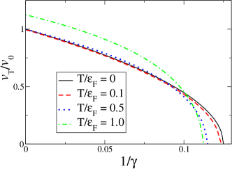
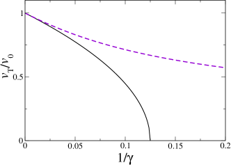
Figure 1: (Color online) (a) The isothermal speed of sound $v_{\rm T}$ of Eq. (21) versus the inverse coupling constant $\gamma^{-1}$ in the HF approximation for different temperatures. The quantity $v_{0}\equiv\hslash\pi n/m$ is the speed of sound of the TG gas at zero temperature. The speed of sound becomes zero at some critical value of $\gamma$, below which the HF solution becomes unstable (see discussion in Sec. III.) (b) The solid (black) line shows the speed of sound in the HF approximation at $T=0$ given by Eq. (22), and the dashed (violet) line shows the exact speed of sound in the Lieb-Liniger model lieb63:2 for comparison.

IV The random phase approximation

IV.1 Response function

The HF approximation permits us to calculate the linear response of time-dependent HF. Approximations of the linear response functions on this level are known as RPA with exchange or generalized RPA pines89 ; pines61 . In this section we will calculate the density-density response function $\chi(q,z)$ also known as dynamic polarizability. It is intimately related to the DSF and the time-dependent density-density correlation function pines89 ; pines61 ; pitaevskii03:book . In order to define $\chi(q,z)$ we consider the linear response of the density

$${n}(x,t)-n=\langle{\hat{\Psi}}^{\dagger}(x,t){\hat{\Psi}}(x,t)\rangle-{n}=\frac{1}{L}\sum_{q}e^{iqx}\delta{n}(q,t)$$

to an infinitesimal time-dependent external potential

$$\delta V_{\mathrm{ext}}(x,t)=\sum_{q}\int\hslash\frac{\mathrm{d}\omega}{2\pi}e^{iqx}e^{-i\omega t}e^{\varepsilon t}\delta V_{\mathrm{ext}}(q,\omega).$$

Here we choose $\varepsilon\to+0$ to provide the boundary condition $V_{\mathrm{ext}}(x,t)\to 0$ when $t\to-\infty$. For $q\not=0$ we have

$$\delta{n}(q,t)= \ \sum_{k}\langle\hat{a}^{{\dagger}}_{k-q/2}(t)\hat{a}_{k+q/2}(t)\rangle$$

$$= \ \int\hslash\frac{\mathrm{d}\omega}{2\pi}e^{-i\omega t}e^{\varepsilon t}\delta{n}(q,\omega).$$ (23)

The dynamic polarizability is now defined by

$$\chi(q,\omega+i\varepsilon)\equiv{-\delta n(q,\omega)}/{\delta V_{\mathrm{ext}}(q,\omega)}$$ (24)

and obviously determines the linear density response to an external field.

The polarizability can be obtained directly from the linearized equation of motion of the density operator in the time-dependent HF approximation in the standard way as summarized below.

(i) With the help of the HF Hamiltonian (10) we write the equation of motion $i\hslash\partial\hat{\rho}^{(1)}/\partial t=[\hat{\rho}^{(1)},\hat{H}_{0}]$ for the operator $\hat{\rho}^{(1)}\equiv{\hat{\Psi}}^{\dagger}(y,t){\hat{\Psi}}(z,t)$ and take its average. We thus derive

$$i\hslash\frac{\partial{\rho}^{(1)}(y,z,t)}{\partial t}=\int\mathrm{d}x\,\big{[} F(z,x){\rho}^{(1)}(y,x,t)$$

$$-F(x,y){\rho}^{(1)}(x,z,t)\big{]}$$ (25)

with the HF kernel $F$ of Eq. (11).

(ii) We substitute ${\rho}^{(1)}(y,z,t)={\rho}^{(1)}_{0}(y-z)+\delta{{\rho}^{(1)}}(y,z,t)$ into Eq. (25) and linearize it with respect to $\delta{\rho}^{(1)}$ and $\delta V_{\mathrm{ext}}$. Here we introduce the equilibrium value of the one-body density matrix ${\rho}^{(1)}_{0}(y-z)=(1/L)\sum_{k}n_{k}\exp[ik(y-z)]$ in the HF approximation with the HF occupation numbers $n_{k}$ of Eq. (13).

(iii) In the Fourier representation of momentum and frequency, the obtained linearized equation becomes algebraic and takes the form

$$\delta\tilde{\rho}^{(1)}(k,q,\omega)\bigg{(}\frac{1}{L}\!\sum_{p}\!n_{p}\big{[}\mathcal{V}(k-p-q/2)-\mathcal{V}(k-p+q/2)\big{]}$$

$$\phantom{\delta\tilde{\rho}^{(1)}(k,q,\omega)\bigg{(}}+\frac{\hslash^{2}kq}{m}-\hslash\omega-i\varepsilon\bigg{)}$$

$$=\bigg{(}\delta V_{\mathrm{ext}}(q,\omega)+\frac{1}{L}\sum_{p}\big{[}\mathcal{V}(q)-\mathcal{V}(p-k)\big{]}\delta\tilde{\rho}^{(1)}(p,q,\omega)\bigg{)}$$

$$\phantom{=}\ \times(n_{k+q/2}-n_{k-q/2}).$$ (26)

Here, $\mathcal{V}(q)=g_{\mathrm{F}}q^{2}$ stands for the Fourier transform of the potential (8) and $\delta\tilde{\rho}^{(1)}$ is defined by the relation $\langle\hat{a}^{{\dagger}}_{k-q/2}(t)\hat{a}_{k+q/2}(t)\rangle=(\hslash/{2\pi})\int\mathrm{d}\omega e^{-i\omega t}e^{\varepsilon t}\delta\tilde{\rho}^{(1)}(k,q,\omega)$ for $q\not=0$. We are interested in the density response $\delta n(q,\omega)$, which is directly connected to $\delta\tilde{\rho}^{(1)}$ by

$$\delta n(q,\omega)=\sum_{k}\delta\tilde{\rho}^{(1)}(k,q,\omega).$$ (27)

Because $\mathcal{V}(q)$ is a polynomial in $q$, we can obtain an analytical expression for the polarizability (24) from Eqs. (26) and (27). After somewhat lengthy but straightforward calculations we find

$$\chi(q,z)=\frac{\chi^{(0)}(q,z)}{(1-4\gamma^{-1})[B+D(q,z)\chi^{(0)}(q,z)]}$$ (28)

with $z\equiv\omega+i\varepsilon$ and $\varepsilon{\to}+0$. Here we denote

$$B\equiv\ 1-{4\,(3\,\gamma-16)}/{(\gamma-4)^{3}},$$

$$D(q,z)\equiv\ \frac{4\varepsilon_{\mathrm{F}}}{N}\frac{\gamma}{(\gamma-4)^{2}}\Bigg{[}\frac{q^{2}}{k_{\mathrm{F}}^{2}}\frac{2\gamma-9}{2\gamma}-\frac{6}{\gamma}\frac{\langle q^{2}\rangle}{k_{\mathrm{F}}^{2}}$$

$$-\left(\frac{\hslash zk_{\mathrm{F}}}{\varepsilon_{\mathrm{F}}q}\right)^{2}\frac{3\gamma-16}{2(\gamma-4)^{2}}\Bigg{]},$$

and the polarizability $\chi^{(0)}$ of the ideal 1D Fermi gas with renormalized mass is given by the relation

$$\chi^{(0)}(q,z)=\sum_{k}\frac{n_{k+q/2}-n_{k-q/2}}{\hslash z-{\hslash^{2}kq}/{m^{*}}}.$$ (29)

In the thermodynamic limit we find the real and imaginary parts of $\chi^{(0)}(q,\omega+i\varepsilon)=\chi^{(0)}_{1}(q,\omega)+i\chi^{(0)}_{2}(q,\omega)$ using the relation $1/(x+i\varepsilon)={\rm P}({1}/{x})-i\pi\delta(x)$

$$\chi^{(0)}_{1}(q,\omega)= \ \frac{Nm^{*}}{2\hslash^{2}qk_{\mathrm{F}}}\,{\rm P}\int\mathrm{d}k\,\frac{n_{k+q_{-}}-n_{k+q_{+}}}{k},$$ (30)

$$\chi^{(0)}_{2}(q,\omega)= \ \frac{Nm^{*}}{2\hslash^{2}qk_{\mathrm{F}}}\pi(n_{q_{-}}-n_{q_{+}}),$$ (31)

where ${\rm P}$ means the Cauchy principal value and we defined

$$q_{\pm}\equiv\frac{\omega m^{*}}{\hslash q}\pm\frac{q}{2}.$$ (32)

At zero temperature the occupation numbers $n_{k}$ define the Fermi step function and we arrive at the simple analytic expressions

$$\chi^{(0)}_{1}(q,\omega)=\ \frac{Nm^{*}}{2\hslash^{2}qk_{\mathrm{F}}}\ln\left|\frac{\omega^{2}_{+}(q)-\omega^{2}}{\omega^{2}_{-}(q)-\omega^{2}}\right|,$$ (33)

$$\chi^{(0)}_{2}(q,\omega)=\ \frac{N\pi m^{*}}{2\hslash^{2}qk_{\mathrm{F}}}\left\{\begin{array}[]{ll}\pm 1,&\omega_{-}\leqslant\pm\omega\leqslant\omega_{+},\\[5.69054pt] 0,&\text{otherwise.}\end{array}\right.$$ (36)

The dispersion relations

$$\omega_{\pm}(q)\equiv{\hslash|2k_{\mathrm{F}}q\pm q^{2}|}/{(2m^{*})}$$ (37)

border the continuum part of the accessible excitation spectrum made up from HF quasiparticle-quasihole excitations (16), as shown in Fig. 2. The two branches $\omega_{\pm}(q)$ thus approximate the two branches of elementary excitations introduced by Lieb lieb63:2 as type I and type II excitations, respectively.

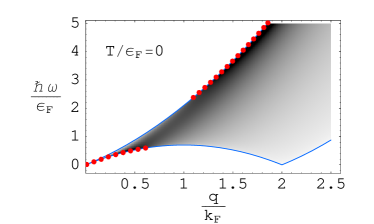
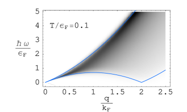
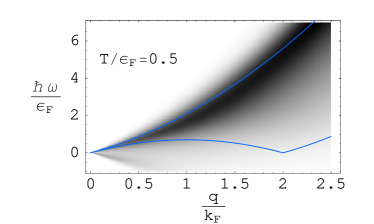
Figure 2: (Color online) The excitation spectrum and the DSF at $\gamma=13$ for various temperatures. The upper and lower thin (blue) lines show the dispersions $\omega_{+}(q)$ and $\omega_{-}(q)$ of Eq. (37), respectively, limiting the elementary excitations of the Lieb-Liniger model at $T=0$. The dimensionless value of the rescaled DSF $S(q,\omega)q\varepsilon_{F}/(k_{\mathrm{F}}N)$ from Eqs. (42) and (45) is shown in shades of grey between zero (white) and 1.0 (black). Here $k_{\mathrm{F}}=\pi n$ and $\varepsilon_{\mathrm{F}}=\hslash^{2}k_{\mathrm{F}}^{2}/(2m)$. The dotted (red) line indicates a $\delta$-function contribution at $\omega_{0}(q)$. At non-zero temperatures the $\delta$-function contribution washes out and becomes a part of the continuum.

In accordance with the exact results, both branches share the same slope at the origin and give rise to a single speed of sound at zero temperature given by $v_{\rm T}={\mathrm{d}\omega_{\pm}}/{\mathrm{d}k}={\hslash k_{\mathrm{F}}}(1-4\gamma^{-1})/{m}$. This value is the correct first order expansion lieb63:2 of $v_{\rm T}$ for large $\gamma$, consistent with Eq. (22). Note that the usual Bogoliubov perturbation theory bog47 for weakly interacting bosons gives a similar expansion of $v_{\rm T}$ for small $\gamma$ and the type I excitation branch. Type II excitations are not described with Bogoliubov theory. The dispersion curves $\omega_{\pm}(q)$ of Eq. (37) differ from the free Fermi gas (TG gas) values only by the renormalization of the mass, which already takes place in the HF single-particle energies.

IV.2 Dynamic structure factor

The DSF $S(q,\omega)$ is the Fourier transform of the density-density correlation function pines89 ; pines61 ; pitaevskii03:book and expresses the probability to excite a particular excited state through a density perturbation

$$S(q,\omega)={\cal Z}^{-1}\sum_{n,m}e^{-\beta E_{m}}|\langle m|\hat{\rho}_{q}|n\rangle|^{2}\delta(\hslash\omega-E_{n}+E_{m}),$$ (38)

where $\hat{\rho}_{q}=\sum_{i}\exp(-iqx_{i})$ is the Fourier component of the density operator, ${\cal Z}=\sum_{n}\exp(-\beta E_{n})$ is the partition function.

The DSF is related to the dynamic polarizability by

$$\chi(q,\omega+i\varepsilon)=\int_{-\infty}^{+\infty}\mathrm{d}\omega^{\prime}\frac{2\omega^{\prime}S(q,\omega^{\prime})}{{\omega^{\prime}}^{2}-(\omega+i\varepsilon)^{2}}$$ (39)

or, equivalently pitaevskii03:book , by

$$S(q,\omega)=\frac{\mathop{\mathrm{Im}}\chi(q,\omega+i\varepsilon)}{\pi[1-\exp(-\beta\hslash\omega)]},$$ (40)

which gives at zero temperature

$$S(q,\omega)=\left\{\begin{array}[]{ll}\mathop{\mathrm{Im}}\chi(q,\omega+i\varepsilon)/\pi,&\omega>0,\\ 0,&\omega<0.\par\end{array}\right.$$ (41)

IV.2.1 Zero temperature

The DSF at zero temperature can be obtained from Eqs. (28) and (41), which result in

$$S(q,\omega)= \frac{\chi^{(0)}_{2}(q,\omega)B}{\pi(1-4\,\gamma^{-1})\left[\Big{(}B+D\chi_{1}^{(0)}\Big{)}^{2}+\Big{(}D\chi_{2}^{(0)}\Big{)}^{2}\right]}$$

$$+\delta[\omega-\omega_{0}(q)]A(q)/\hslash,$$ (42)

with $\chi^{(0)}_{1,2}$ given by the zero temperature expressions (33) and (36). A grey scale plot of this result is shown in Fig. 2. The DSF of Eq. (42) has two contributions. The first part is continuous and takes nonzero (and positive) values only for $\omega_{-}<\omega<\omega_{+}$, which is also the region where particle-hole excitations on the HF level are present. The second part is a discrete branch with strength $A(q)$ and located at $\omega=\omega_{0}(q)$, outside the region of the discrete contribution. As we will discuss in detail below, the discrete part is exponentially suppressed for small $\gamma^{-1}$ and should be understood as an artefact of the RPA approximation.

Due to a logarithmic singularity in $\chi_{1}^{(0)}$, the DSF vanishes on the dispersion curves $\omega_{\pm}(q)$. For the TG gas at $\gamma\to\infty$, the value of the DSF within these limits is independent of $\omega$ and takes the value of $Nm/(2\pi\hslash^{2}qn)$. The energy-dependence in the RPA for finite $\gamma^{-1}$ is shown in Figs. 2 and 3. In particular, we see that the umklapp excitations at $q=2k_{\mathrm{F}}$ and small $\omega$, which prohibit superfluidity of the TG gas, are suppressed for finite $\gamma$. We find that $S(2k_{\mathrm{F}},\omega)$ in the RPA approaches zero as $1/\ln^{2}(\hslash\omega/\varepsilon_{\mathrm{F}})$, in contrast to the results of Refs. castro_neto94 ; pitaevskii04 , which predict a power-law dependence on $\omega$ for finite $\gamma$ based on a pseudoparticle-operator approach.

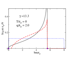
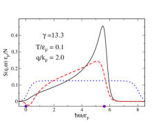
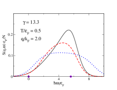
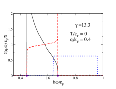
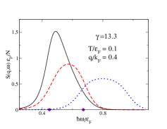
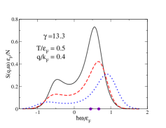
Figure 3: (Color online) The DSF $S(q,\omega)\,\varepsilon_{\mathrm{F}}/N$ at interaction strength $\gamma=13.33$ as a function of $\omega$ at $q=0.4k_{\mathrm{F}}$ and $q=2k_{\mathrm{F}}$ for various temperatures. The solid (black) line shows the RPA result (42) or (45), the dashed (red) line shows the first order expansion in $\gamma^{-1}$ (43) or (IV.2.2), and the dotted (blue) line shows the DSF of the TG limit ($\gamma=\infty$) for comparison. The circular (violet) dots on the x-axis denote $\omega_{\pm}$. The first-order expansion always has a divergence to $\pm\infty$ near $\omega_{\pm}$ at $T=0$, respectively, and the maximum is shifted to $\omega_{+}$ at finite $T$. The RPA result, however, shows an enhancement of low-energy excitation near $\omega_{-}$ at small $q$. Note the unphysical negative values of the DSF in the first order expansion near $\omega_{-}$, in particular for the umklapp excitations at $q=2k_{\mathrm{F}}$ and $\omega$ close to zero.

In the RPA the enhancement of Bogoliubov-like excitations is seen as a strong and narrow peak of the DSF in the RPA near $\omega_{+}$ at large momenta in Fig. 3. At finite gamma and for small momenta $q\lesssim\pi n/2$, however, the RPA predicts a peak near $\omega_{-}$, in contrast to the first-order result. Whether this effect is real or an artefact of the RPA is not obvious and may be decided by more accurate calculations or experiments. Spurious higher order terms in the RPA and an improved approximation scheme have been discussed in Ref. brand98 . On the other hand, Roth and Burnett have recently observed a qualitatively similar effect in numerical calculations of the DSF of the Bose-Hubbard model roth04 .

The RPA result may be expanded in $1/\gamma$, which is consistent with direct perturbation theory up to first order. This yields for $\omega_{-}\leqslant\omega\leqslant\omega_{+}$

$$S(q,\omega)\frac{\varepsilon_{\mathrm{F}}}{N}=k_{\mathrm{F}}\frac{1+8\gamma^{-1}}{4q}+\frac{\ln f(q,\omega)}{2\gamma}+{\cal O}(\gamma^{-2})$$ (43)

with $f(q,\omega)\equiv|(\omega^{2}-\omega_{-}^{2})/(\omega_{+}^{2}-\omega^{2})|$. However, this first order expansion can assume negative values as seen in Fig. 3 although the DSF, given by Eq. (38), should be strictly non-negative, a property that our RPA result (42) fulfills. Close to $\omega_{+}$, the first order expansion has a logarithmic singularity tending to $+\infty$, which may be a precursor of the dominance of Bogoliubov-like excitations in the DSF at small $\gamma$. In the TG limit $\gamma^{-1}=0$, the DSF becomes discontinuous with respect to $\omega$ at $\omega_{\pm}$ because the DSF of the TG gas is a step function [see Eq. (36)]. As a consequence, the first order approximation (43) cannot be good for arbitrary values of $q$ and $\omega$ but diverges in vicinity of $\omega_{\pm}$ due to the slow convergence of perturbation theory close to the point of discontinuity. There is no formal problem here since the expression (43) remains positive if for any given finite value of $q$ and $\omega\not=\omega_{-}$ a large enough value of gamma is chosen.

Finally we discuss the $\delta$-function part of the DSF (42). This contribution relating to discrete excitations of collective character in the time-dependent HF scheme lies outside of the continuum part and comes from possible zeros in the denominator of $\chi(q,\omega+i\varepsilon)$. It is determined by the solution $\omega_{0}(q)$ of the transcendental equation $B=-D(q,\omega)\chi_{1}^{(0)}(q,\omega)$ in conjunction with $\chi_{2}^{(0)}(q,\omega)=0$. We have solved this equation in various limits and found that at most one solution for $\omega_{0}(q)$ exists. The strength $A(q)$ is given by the residue of the polarizability at the pole $z_{0}=\omega_{0}(q)$. After small algebra, we derive from Eq. (28)

$$A(q)=N\frac{(\gamma-4)^{3}}{4(3\gamma-4)}\frac{\varepsilon_{\mathrm{F}}}{\hslash\omega_{0}(q)}\frac{\eta^{2}}{1+16\eta^{2}h_{0}},$$ (44)

where $\eta\equiv q/k_{\mathrm{F}}$ and

$$h_{0}\equiv\frac{\gamma(\gamma-6)^{2}}{3\gamma-4}\frac{\big{[}\ln|\xi-(\eta-2)^{2}|-\ln|\xi-(\eta+2)^{2}|\big{]}^{-1}}{[\xi-(\eta-2)^{2}][\xi-(\eta+2)^{2}]}$$

with $\xi\equiv[\hslash\omega_{0}(q)/\varepsilon_{\mathrm{F}}]^{2}\gamma^{2}/[\eta(\gamma-4)]^{2}$.

Numerical values for $A(q)\omega_{0}(q)$ are shown at finite $\gamma$ in Fig. 4. For small $q$ we find a $\delta$-function contribution at $\omega_{0}(q)<\omega_{-}$ whereas for large $q$ there is a discrete contribution at $\omega_{0}(q)>\omega_{+}$ (see Fig. 2a). In the limit $q\to\infty$ at finite $\gamma$, the $\delta$-part completely determines the DSF as the continuum part vanishes; asymptotically $A\simeq N$, and $\omega_{0}\simeq\hslash q^{2}/(2m)$ becomes the free particle dispersion, reminiscent of the DSF for the weakly interacting Bose gas at large momentum in Bogoliubov theory bog47 .

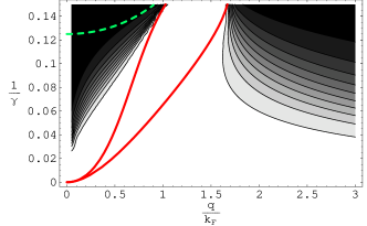
Figure 4: (Color online) Contour plot of $A(q)\,2m\omega_{0}(q)/(\hslash Nq^{2})$, which shows the importance of the $\delta$-function contribution. Values are given in ten contours between 0 (white) and 1 (black). Between the thick (red) lines there is no discrete contribution because $\chi$ given by Eq. (28) has no poles. Left of this region, there is a discrete part with $\omega_{0}<\omega_{-}$ and right of it there is one with $\omega_{0}>\omega_{+}$. Above the dashed (green) line the RPA breaks down due to an instability of the HF ground state as discussed in Sec. III.

For small $\gamma^{-1}$, the strength $A(q)\simeq 2N\gamma\exp(-\gamma q/k_{\mathrm{F}})$ is exponentially suppressed and possible solutions are close to the dispersion branches $\omega_{\pm}$ with $|\omega_{0}-\omega_{\pm}|\propto\exp(-\gamma q/k_{\mathrm{F}})$. Due to this proximity of the discrete and continuous parts and expected smearing of discrete contributions by interactions beyond the RPA, we may conjecture that the $\delta$-function should be seen as part of the continuum, enhancing contributions near the border. Moreover, at finite temperatures there is no $\delta$-function contribution even within the RPA, as we discuss in Sec. IV.2.2 below. Indeed, we know from the exact solutions lieb63:2 that the energy spectrum is continuous.

The RPA polarizability (28) is a retarded Green’s function and thus has to be analytic in the upper half complex plane pines89 ; pines61 . At zero temperature, the analyticity breaks down above the dashed (green) line in Fig. 4. The instability of the RPA results from the instability of the HF approximation thouless61 and arises exactly at the critical value of $\gamma$ when the isothermal speed of sound equals to zero, see Fig. 1.

IV.2.2 Finite temperatures

At finite temperatures we obtain the DSF by means of Eqs. (28) and (40)

$$S(q,\omega)=\frac{\chi^{(0)}_{2}(q,\omega)B[1-\exp(-\beta\hslash\omega)]^{-1}}{\pi(1-4\,\gamma^{-1})\left[\Big{(}B+D\chi_{1}^{(0)}\Big{)}^{2}+\Big{(}D\chi_{2}^{(0)}\Big{)}^{2}\right]},$$ (45)

where the real and imaginary parts of the polarizability $\chi^{(0)}_{1,2}$ are given by Eqs. (30) and (31), respectively. The DSF is shown in Figs. 2 and 3. The main effect of finite temperature is a smoothing of the zero-temperature features. The $\delta$-function contribution to the DSF disappears, since $\chi_{2}^{(0)}\not=0$ and thus the denominator of Eq. (45) does not vanish for $\omega\not=0$. It is absorbed by the continuum part of the DSF.

At finite temperatures, the non-vanishing contributions of the DSF spread considerably beyond the particle-hole excitation spectrum limited by $\omega_{-}$ and $\omega_{+}$ because the DSF no longer probes the ground state but a thermal ensemble [see Eq. (38)]. For negative values of the frequency, the DSF decays exponentially in accordance with Eq. (40). Similar to the case of zero temperature, the enhancement of excitations still takes place close to $\omega_{+}$ for $q\gtrsim\pi n/2$ and $\omega_{-}$ for $q\lesssim\pi n/2$ at small values of temperature $T\lesssim 0.5\varepsilon_{\mathrm{F}}$.

To the first order in $\gamma^{-1}$, we have

$$S(q,\omega)\frac{\varepsilon_{\mathrm{F}}}{N}= \ \frac{n_{q_{-}}-n_{q_{+}}}{1-\exp(-\beta\hslash\omega)}\bigg{[}k_{\mathrm{F}}\frac{1+8\gamma^{-1}}{4q}$$

$$\ +\frac{1}{2\gamma}{\rm P}\int\mathrm{d}k\,\frac{n_{k+q_{+}}-n_{k+q_{-}}}{k}\bigg{]}+{\cal O}(\gamma^{-2}).$$ (46)

This linear approximation fails in vicinity of the umklapp excitation $q=2k_{\mathrm{F}}$ and $\omega=0$, yielding unphysically negative values of the DSF contrary to the obtained RPA expression (45), see Fig. 3.

IV.2.3 Sum rules for the DSF

Sum rules for the DSF are an important test for checking the validity of the obtained expressions. In particular, the $f$-sum rule pitaevskii03:book ; pines61 ; pines89

$$m_{1}\equiv\hslash^{2}\int\omega S(q,\omega)\mathrm{d}\omega=N\hslash^{2}q^{2}/(2m)$$ (47)

should be fulfilled to all orders in $\gamma^{-1}$ within the RPA thouless61 . We have verified it by numerical integration and found excellent agreement at finite values of $\gamma$ for both the zero-temperature DSF (42) and the finite temperature expression (45). The $f$-sum rule can also be verified analytically from the large $\omega$ asymptotics $\chi(q,\omega)\simeq-2m_{1}/(\hslash\omega)^{2}$ using Eqs. (28) and (39), assuming that $\chi$ is analytic as a function of $\omega$ in the upper half complex plane.

The sum rule for the isothermal compressibility pitaevskii03:book

$$\lim_{q\to 0}{\rm P}\int\frac{S(q,\omega)}{\omega}\mathrm{d}\omega=\frac{N}{2n}\Big{(}\frac{\partial n}{\partial\mu}\Big{)}_{T}$$ (48)

holds also to all orders in $\gamma^{-1}$, which can be checked analytically. Indeed, by comparing Eq. (28) with the HF isothermal compressibility discussed in Sec. III we derive

$$\lim_{q\to 0}\chi(q,0+i\varepsilon)=\frac{N}{n}\Big{(}\frac{\partial n}{\partial\mu}\Big{)}_{T}.$$ (49)

Then Eq. (48) is a direct consequence of the dispersion relation (39) at $\omega=0$.

IV.2.4 Consequences for superfluidity

As we have argued in Ref. brand05 , the value of the DSF near the umklapp excitations at $\omega=0$ and $q=2k_{\mathrm{F}}$ is relevant for the phenomenon of superfluidity according to the Landau criterion. A finite value of $S(q,\omega)$ will prohibit persistent currents, as spontaneous excitations initiated by infinitesimal perturbations would be able to dissipate the translational kinetic energy stored in the current. Our finite temperature results clearly show that $S(q=2k_{\mathrm{F}},\omega=0)$ at a given value of $T>0$ will always be positive and finite for large enough $\gamma$ in both the RPA expression (45) and the first order expansion (IV.2.2). We thus conclude that there is no superfluidity in the large-$\gamma$ regime at finite temperatures, in accordance with Popov’s analysis popov72 made many years ago. The question of efficient suppression of the DSF in the vicinity of the umklapp excitation at $T=0$ cannot be fully answered within the present approach due to the nonregularity of $S(q,\omega)$ at this point, as discussed in Ref. brand05 , and will be left to future investigations.

IV.3 Static structure factor and pair distribution function

The static structure factor $S(q)$ pitaevskii03:book ; pines61 ; pines89 is a function of momentum only and is obtained by integrating the DSF over the frequency

$$S(q)\equiv\frac{\langle\hat{\rho}_{q}\hat{\rho}^{{\dagger}}_{q}\rangle}{N}=\frac{\hslash}{N}\int\mathrm{d}\omega\,S(q,\omega).$$ (50)

The results of numerical integration of the DSF in the RPA are plotted in Fig. 5.

The static structure factor contains information about the static correlation properties of a system and directly relates to the pair distribution function or the normalized density-density correlator $g(x)\equiv\langle{\hat{\Psi}}^{\dagger}(x){\hat{\Psi}}^{{\dagger}}(0){\hat{\Psi}}(0){\hat{\Psi}}(x)\rangle/n^{2}$ by the equation

$$g(x)=1+\int\frac{\mathrm{d}q}{2\pi n}\,e^{iqx}\big{[}S(q)-1\big{]}.$$ (51)

At small momenta $S(q)$ can be related to the isothermal compressibility because the main contribution into the integral (50) comes from the “classical” region $\hslash\beta\omega\ll 1$ pitaevskii03:book . We derive from Eqs. (39), (40), (49), and (50)

$$\lim_{q\to 0}S(q)=\frac{T}{n}\Big{(}\frac{\partial n}{\partial\mu}\Big{)}_{T}=\frac{T}{mv^{2}_{\rm T}}.$$ (52)

This relation of the structure factor $S(q)$ to the speed of sound $v_{\rm T}$ at small momentum implies that $S(q)$ in the RPA is exact up to first order in $\gamma^{-1}$ and is overestimated at finite $\gamma$ as seen from the results for $v_{\rm T}$ in Fig. 1.

IV.3.1 Zero temperature

We can obtain the static structure factor (50) from Eq. (43) to the first order

$$S(q)=S^{(0)}(q)+\gamma^{-1}S_{1}(q)+\mathcal{O}(\gamma^{-2}).$$ (53)

Here $S^{(0)}$ denotes the static structure factor for the ideal 1D Fermi gas

$$S^{(0)}(q)=\left\{\begin{array}[]{ll}|q|/(2k_{\mathrm{F}}),&|q|\leqslant 2k_{\mathrm{F}},\\[5.69054pt] 1,&|q|\geqslant 2k_{\mathrm{F}},\end{array}\right.$$ (54)

and the function $S_{1}(q)$ takes the form

$$S_{1}(q)=\ |\eta|\big{[}r(\eta)-|\eta-2|\ln|\eta-2|-|\eta+2|\ln|\eta+2|\big{]}$$

$$\ +4S^{(0)}(q)$$ (55)

with the dimensionless wave vector $\eta\equiv q/k_{\mathrm{F}}$ and the function

$$r(\eta)\equiv\left\{\begin{array}[]{ll}4\ln 2,&|\eta|\leqslant 2,\\[5.69054pt] 2|\eta|\ln|\eta|,&|\eta|\geqslant 2.\end{array}\right.$$ (56)

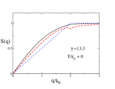
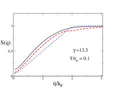
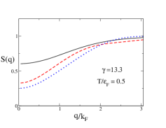
Figure 5: (Color online) The static structure factor $S(q)$ as a function of momentum for $\gamma=13.3$ and various temperatures. The solid (black) line shows the RPA result obtained by numerical integration from Eqs. (42) or (45). The dashed (red) line shows the first order expansion (53) in $\gamma^{-1}$ with Eqs. (54) and (55) at zero temperature or Eqs. (59) and (60) at non-zero temperatures. The dotted (blue) line shows the static structure factor in the TG limit ($\gamma=\infty$) (54) or (59) for comparison. Note the unphysical cusp at $q=2k_{\mathrm{F}}$ in the first-order expansion of the static structure factor at zero temperature and some traces of it at small temperature.

The obtained correction $S_{1}(q)$ is continuous and has the asymptotics $S_{1}(q)\simeq-8/(3\eta^{2})+\mathcal{O}(1/\eta^{4})$ when $\eta\to\infty$ and $S_{1}(q)\simeq 2|\eta|-|\eta|^{3}/2+\mathcal{O}(\eta^{5})$ when $\eta\to 0$. The latter asymptotics gives us a possibility to determine the coupling constant $\gamma$ experimentally from the phonon part of the static structure factor (53) for $q\lesssim k_{\mathrm{F}}$

$$S(q)\simeq\frac{|q|}{2k_{\mathrm{F}}}\bigg{(}1+\frac{4}{\gamma}-\frac{q^{2}}{\gamma k_{\mathrm{F}}^{2}}\bigg{)}.$$ (57)

The static structure factor at small $q$ is related to the sound velocity pitaevskii03:book by $S(q)\simeq{\hslash|q|}/{(2mv_{\rm T})}$. It is easily seen that our result (57) is consistent with the sound velocity of Eq. (22).

Figure 5 shows the static structure factor in the full RPA and its first order expansion (53) at $\gamma=13.3$ and the TG limit $S^{(0)}$ for comparison. The first order result shows a cusp which is an artefact of the first order expansion.

Using Eq. (51) in conjunction with relations (53)-(56), we can represent our result for the pair distribution function in the form

$$g (x)=\ 1-\frac{\sin^{2}z}{z^{2}}-\frac{2\pi}{\gamma}\frac{\partial}{\partial z}\frac{\sin^{2}z}{z^{2}}-\frac{4}{\gamma}\frac{\sin^{2}z}{z^{2}}$$

$$+\frac{2}{\gamma}\frac{\partial}{\partial z}\left[\frac{\sin z}{z}\int_{-1}^{1}\mathrm{d}\eta\,\sin(\eta z)\ln\frac{1+\eta}{1-\eta}\right]+\mathcal{O}(\gamma^{-2}),$$ (58)

where $z=k_{\mathrm{F}}x=\pi nx$. It follows from this equation that $g(x=0)$ vanishes not only in the TG limit but also in first order of $\gamma^{-1}$, which is consistent with the results of Refs. lieb63:1 ; Gangardt2003a and the HF expression (62) below, indicating once more the validity of our results. The physically correct limit $g(x)\to 1$ for $x\to\infty$ is fulfilled due to Eq. (51). A similar expression for $g(x)$ was derived in Ref. korepin93 for the large distance asymptotics. To our knowledge, Eq. (58) shows for the first time the full $x$ dependence of $g(x)$ up to first order in $\gamma^{-1}$.

IV.3.2 Finite temperatures

The first-order approximation for the static structure factor at finite temperatures is obtained by using Eqs. (IV.2.2) and (50). The result takes the form of Eq. (53) but with the TG, or free Fermi, static structure factor

$$S^{(0)}(q)=\frac{m}{2\hslash k_{\mathrm{F}}q}\int\mathrm{d}\omega\frac{n_{q_{-}}-n_{q_{+}}}{1-\exp(-\beta\hslash\omega)}$$ (59)

and with the function $S_{1}(q)$

$$S_{1}(q)\!= \frac{m}{\hslash k_{\mathrm{F}}^{2}}\int\mathrm{d}\omega\frac{n_{q_{-}}-n_{q_{+}}}{1-\exp(-\beta\hslash\omega)}{\rm P}\!\int\mathrm{d}k\,\frac{n_{k+q_{+}}-n_{k+q_{-}}}{k}$$

$$+4S^{(0)}(q),$$ (60)

where $q_{\pm}$ is given by Eq. (32) at $\gamma^{-1}=0$. The finite temperature results are plotted in Fig. 5. One can see an unphysical behaviour of the first order approximation near $q=2k_{\mathrm{F}}$, in contrast to the full RPA result. The small momentum limits for $S(q)$ are determined by the speed of sound $v_{\rm T}$ through Eq. (52). In the plot on the right hand side, the RPA overestimates $S(q)$ at small $q$ as a result of the deviations of the speed of sound as seen in Fig. 1.

IV.3.3 Limits of validity

When the interaction is proportional to a small parameter, the RPA method is applicable and yields correct values of the DSF at least up to the first order in this parameter pines89 ; pines61 ; thouless72 . This implies the validity of the obtained expressions for the polarizability, the dynamic and static structure factors, and the pair distribution function up to the first order in $\gamma^{-1}$. Smallness of the inverse coupling constant means, in particular, small values of the pair distribution function in the contact point: $g(x=0)\ll 1$, which is the TG regime by definition.

A classification of different regimes in the 1D Bose gas for arbitrary temperatures was given in Ref. Shlyapnikov2003 . As it was mentioned above, it is possible to obtain the values of $g(x)$ at $x=0$ from the exact solution of the Lieb-Liniger model with the help of the Hellmann-Feynman theorem. The TG regime is realized Shlyapnikov2003 when

$$\gamma\gg\text{max}(1,\sqrt{T/\varepsilon_{\mathrm{F}}}),$$ (61)

which gives also the criterion of validity of the RPA results. We can derive this criterion within the HF approach of Sec. III. Indeed, we obtain the following result for the pair distribution function by applying the Hellmann-Feynman theorem to the HF grand potential $\Omega$:

$$g(x=0)=\frac{4\pi^{2}}{\gamma^{2}}\frac{\langle k^{2}\rangle}{k_{\mathrm{F}}^{2}}.$$ (62)

Using the low-temperature expansion of the average momentum (18) $\langle k^{2}\rangle=(k_{\mathrm{F}}^{2}/{3})[1+\pi^{2}T^{2}/(4\varepsilon_{\mathrm{F}}^{2})+\cdots]$ and the high-temperature expansion $\langle k^{2}\rangle=k_{\mathrm{F}}^{2}T/[2\varepsilon_{\mathrm{F}}(1-4\gamma^{-1})]+\cdots$, we arrive at the above mentioned restriction on $\gamma$.

The validity of the RPA requires, in particular, the stability of the HF solutions thouless61 . Thus our results are applicable in practice for $\gamma\gtrsim 10$, see discussion in Sec. III.

Note that the HF expression (62) yields the correct value of the pair distribution function only at $x=0$ but up to the second order in $\gamma^{-1}$. This is due to validity of the HF approximation in the first order in $1/\gamma$; hence, the derivative with respect to $\gamma$ of the first-order correction for the grand potential gives the correct value of $g(x=0)$, proportional to $1/\gamma^{2}$. By contrast, the RPA expression (58) and its finite temperature generalization yield the values of $g(x)$ for arbitrary $x$ but guarantee validity only up to the first order. For this reason, the numerical values of $g(x=0)$ obtained with Eqs. (45), (50), and (51) differ from those of Eq. (62).

V Conclusion

We have derived variational approximations for the dynamic polarizability and related two-particle correlation functions of the one-dimensional Bose gas, extending our previous results brand05 to finite temperatures. The approximations are good for strong interactions and yield expansions valid to first oder in $1/\gamma$, which had not been available previously. We have carefully checked the consistency with known limits and sum rules and analyzed the limits of validity of the derived equations. Due to the Bose-Fermi duality, our results are equally applicable for strongly interacting bosons as well as for weakly-interacting spinless fermions. Our result for the DSF indicates a dramatic departure from the TG limit already for very small values of $1/\gamma$ by enhancing Bogoliubov-like excitations and by suppressing umklapp excitation, which are the main obstacle to observing superfluid-like response in the 1D Bose gas. However, we find that superfluidity at finite temperatures is strictly prohibited in the large-$\gamma$ regime as umklapp excitations are always associated with a finite probability. Finite temperature effects generally are found to smear out the sharp features of the zero temperature correlation functions. Nevertheless, at a level of 10% of the Fermi temperature $\varepsilon_{\rm F}$, the main effects should be well observable in experiments.

Our results also establish the usefulness and validity of the fermionic pseudopotentials (8) and (4) and the variational Hartree-Fock approximation and RPA. The method can easily be extended to further studies in the large-$\gamma$ regime by including the effects of harmonic or periodic external potentials or by studying nonlinear response properties. Furthermore, the acquired knowledge of the dynamic density correlations will be useful for constructing an accurate time-dependent density functional theory, extending the approach of Ref. brand04a .

The authors are grateful to Sungyun Kim and Rashid Nazmitdinov for useful remarks.

References

- (1) E. H. Lieb and W. Liniger, Phys. Rev. 130, 1605 (1963), the Lieb-Liniger parameter relates to our notations by .
- (2) E. H. Lieb, Phys. Rev. 130, 1616 (1963).
- (3) The boson coupling constant is related to the 1D and 3D -wave scattering lengths, and , respectively by , where is the frequency of transverse confinement and . M. Olshanii, Phys. Rev. Lett. 81, 938 (1998) and A. Yu. Cherny and J. Brand, Phys. Rev. A 70, 043622 (2004).
- (4) P. C. Hohenberg, Phys. Rev. 158, 383 (1967).
- (5) E. B. Sonin, Zh. Eksp. Teor. Fiz. 59, 1416 (1970) [Sov. Phys. JETP 32, 773 (1971)].
- (6) Y. Kagan, N. V. Prokof’ev, and B. V. Svistunov, Phys. Rev. A 61, 045601 (2000).
- (7) H. P. Büchler, V. B. Geshkenbein, and G. Blatter, Phys. Rev. Lett. 87, 100403 (2001).
- (8) M. D. Girardeau, J. Math. Phys. 1, 516 (1960); A. Lenard, J. Math. Phys. 5, 930 (1964).
- (9) T. Kinoshita, T. Wenger, and D. S. Weiss, Science 305, 1125 (2004).
- (10) B. Paredes et al., Nature 429, 277 (2004).
- (11) H. Moritz et al., Phys. Rev. Lett. 91, 250402 (2003).
- (12) T. Stöferle et al., Phys. Rev. Lett. 92, 130403 (2004).
- (13) One can argue (see Ch. 12 of Ref. pitaevskii03:book ) that the Bragg scattering gives us the imaginary part of the polarizability rather than the DSF itself. This can be essential at finite temperature. Certainly, knowing one quantity, one can easily calculate the other by relation (40).
- (14) C. N. Yang and C. P. Yang, J. Math. Phys. (N.Y.) 10, 1115 (1969).
- (15) V. E. Korepin, N. M. Bogoliubov, and A. G. Izergin, Quantum Inverse Scattering Method and Correlation Functions (University Press, Cambridge, 1993).
- (16) V. Korepin and N. Slavnov, Phys. Lett. A 236, 201 (1997).
- (17) F. H. L. Eßler, V. E. Korepin, and F. T. Latrémolière, Eur. Phys. J. B 5, 559 (1998).
- (18) D. M. Gangardt and G. V. Shlyapnikov, Phys. Rev. Lett. 90, 010401 (2003).
- (19) D. M. Gangardt and G. V. Shlyapnikov, New J. Phys. 5, 79 (2003).
- (20) K. V. Kheruntsyan, D. M. Gangardt, P. D. Drummond, and G. V. Shlyapnikov, Phys. Rev. Lett. 91, 040403 (2003).
- (21) M. Olshanii and V. Dunjko, New J. Phys. 5, 98 (2003); eprint cond-mat/0210629 (2002).
- (22) G. E. Astrakharchik and S. Giorgini, Phys. Rev. A 68, 031602(R) (2003).
- (23) M. Rigol and A. Muramatsu, Phys. Rev. Lett. 93, 230404 (2004).
- (24) V. V. Cheianov, H. Smith, M. B. Zvonarev, E-print cond-mat/0506609.
- (25) T. Cheon and T. Shigehara, Phys. Rev. Lett. 82, 2536 (1999).
- (26) M. A. Cazalilla, Phys. Rev. A 67, 053606 (2003).
- (27) B. E. Granger and D. Blume, Phys. Rev. Lett. 92, 133202 (2004).
- (28) M. D. Girardeau and M. Olshanii, Phys. Rev. A 70, 023608 (2004).
- (29) H. Grosse, E. Langmann, and C. Paufler, J. Phys. A 37, 4579 (2004).
- (30) K. Kanjilal and D. Blume, Phys. Rev. A 70, 042709 (2004).
- (31) J. Brand and A. Yu. Cherny, Phys. Rev. A 72, 033619 (2005).
- (32) A. Lenard, J. Math. Phys. 5, 930 (1964).
- (33) P. Šeba, Rep. Math. Phys. 24, 111 (1986).
- (34) D. Sen, Int. J. Mod. Phys. 14, 1789 (1999); J. Phys. A 36, 7517 (2003).
- (35) Note that an arbitrary local interaction is associated with the kernel .
- (36) A. Isihara, J. Phys. A 1, 539 (1968).
- (37) D. J. Thouless, The Quantum Mechanics of Many-Body Systems (Academic Press, New York, 1972).
- (38) D. Pines and P. Nozières, The theory of quantum liquids (Addison-Wesley, Redwood City, 1989).
- (39) D. Pines, ed., The many-body problem (W.A. Benjamin, New York, 1961).
- (40) L. Pitaevskii and S. Stringari, Bose-Einstein Condensation (Clarendon, Oxford, 2003).
- (41) N. N. Bogoliubov, J. Phys. (USSR) 11, 23 (1947), reprinted in Ref. pines61 .
- (42) A. H. Castro Neto et al., Phys. Rev. B 50, 14032 (1994).
- (43) G. E. Astrakharchik and L. P. Pitaevskii, Phys. Rev. A 70, 013608 (2004).
- (44) J. Brand and L. S. Cederbaum, Phys. Rev. A 57, 4311 (1998).
- (45) R. Roth and K. Burnett, J. Phys. B 37, 3893 (2004).
- (46) D. J. Thouless, Nucl. Phys. 22, 78 (1961).
- (47) V. N. Popov, Teor. Mat. Fiz. 11, 354 (1972) [Theor. Math. Phys. 11, 565 (1972)].
- (48) J. Brand, J. Phys. B 37, S287 (2004).