Thermodynamics, Structure, and Dynamics of Water
Confined between Hydrophobic Plates

Abstract

We perform molecular dynamics simulations of 512 water-like molecules that interact via the TIP5P potential and are confined between two smooth hydrophobic plates that are separated by 1.10 nm. We find that the anomalous thermodynamic properties of water are shifted to lower temperatures relative to the bulk by $\approx 40$ K. The dynamics and structure of the confined water resemble bulk water at higher temperatures, consistent with the shift of thermodynamic anomalies to lower temperature. Due to this $T$ shift, our confined water simulations (down to $T=220$ K) do not reach sufficiently low temperature to observe a liquid-liquid phase transition found for bulk water at $T\approx 215$ K using the TIP5P potential. We find that the different crystalline structures that can form for two different separations of the plates, $0.7$ nm and $1.10$ nm, have no counterparts in the bulk system, and discuss the relevance to experiments on confined water.

I Introduction

Despite the numerous accomplishments in water research to date pablo-rev ; Debenedetti03a ; Debenedetti03b ; braskin , the topic continues to be the subject of intense interest. In particular, water confined in nanoscale geometries has garnered much recent attention due to its biological and technological importance zangi-rev ; gelb . Confinement can lead to changes in both structural and dynamical properties caused by the interaction with a surface and/or a truncation of the bulk correlation length. Moreover these changes depend on whether the interactions of water with the wall particles are hydrophilic or hydrophobic chandler1 . One of the motivations for studying two different kinds of interactions arises from studies of protein folding, since the folding of a protein is influenced by its hydrophobic and hydrophilic interactions with water protein .

It is not clear exactly how the dynamics of liquids depends on the nature of the confining surfaces. The behavior may change depending on the surface morphology. Simulations of simple liquids show that the dynamics typically slow down near a non-attractive rough surface while the dynamics speed up near a non-attractive smooth surface kb1 . A slowing down of water dynamics near a hydrophilic surface has been experimentally observed bellisent . Water confined in Vycor Chen95 ; Chen94 has at least two different dynamical regimes arising from the slow dynamics of water near the surface and fast dynamics of water far away from the surfaces gallo1 ; Spohr99 ; Gallo00 ; Hartnig00 ; Gallo99 ; Gallo00b .

One anomaly hypothesized to occur in supercooled water is the emergence of a phase transition line separating liquid states of different densities. This phenomenon is called a liquid-liquid (LL) phase transition pses92 ; ms98 ; poole1 ; speh ; slhp ; Sciortino03 . A LL transition has been seen in a variety of simulation models of water masako ; pses92 ; hpss , but is difficult to observe experimentally due to the propensity of ice to nucleate at temperatures where a transition is expected. Nonetheless, indirect evidence of a transition has been found Mishima98 ; ms98 ; chenpaper ; ChenPRVT ; richert . Studies of some simple models of liquid also show a LL phase transition Ja98 ; Bul02 ; Fr01 ; fran02 ; Ku04 .

Bulk water simulations using the TIP5P potential jorgensen1 ; jorgensen2 indicate the presence of a LL phase transition ending in a second critical point at $T\approx 217$ K and $\rho\approx 1.17$ g/cm³ masako ; paschek1 . A LL phase transition has been suggested based on simulations using the ST2 potential confined between smooth plates meyer . A liquid-to-amorphous transition is seen in simulations using the TIP4P potential tip4p ; tip4p-tanaka1 ; tip4p-tanaka2 confined in carbon nanotubes koga2 . Recent theoretical work truskett suggests that hydrophobic confinement suppresses the LL transition to lower $T$. Here we aim to determine how confinement between smooth hydrophobic walls affects the location of the the LL critical point as well as the overall thermodynamic, dynamic and structural properties.

The freezing of water in confined spaces is also interesting. On one hand, recent experimental studies of water confined in carbon nanopores show that water does not crystallize even when the temperature is cooled down to 77 K bellisent . On the other hand, computer simulation studies show that models of water can crystallize into different crystalline forms when confined between surfaces koga1 ; zangi1 ; zangi2 ; tanaka2 ; koga3 . For example, monolayer ice was found in simulations using the TIP5P model of water zangi1 . By applying an electric field along lateral directions (directions perpendicular to the confinement direction) another crystalline structure for three molecular layers of water confined between two silica plates was found zangi2 . Also, bilayer hexagonal ice was found in simulations using the TIP4P model koga1 . In general these simulations predict a variety of polymorphs in confined spaces, but the crystalline structures found have yet to be observed in experiments.

This paper is organized as follows: In Sec. II, we provide details of our simulations and analysis methods. Simulation results for the liquid state are provided in Secs. III, IV, and V. The crystal states are discussed in Sec. VI, and we conclude with a brief summary in Sec. VII.

II Simulation and Analysis Methods

We perform molecular dynamics (MD) simulations of a system composed of $N=512$ water-like molecules confined between two smooth walls. The molecules interact via the TIP5P pair potential jorgensen1 which, like the ST2 st2 potential, treats each water molecule as a tetrahedral, rigid, and non-polarizable unit consisting of five point sites. Two positive point charges of charge $q_{H}=0.241e$ (where $e$ is the fundamental unit of charge) are located on each hydrogen atom at a distance $0.09572$ nm from the oxygen atom; together they form an $HOH$ angle of $104.52^{\circ}$. Two negative point charges ($q_{e}=-q_{H}$) representing the lone pair of electrons ($e^{-}$) are located at a distance $0.07$ nm from the oxygen atom. These negative point charges are located in a plane perpendicular to the $HOH$ plane and form an $e^{-}Oe^{-}$ angle of $\cos^{-1}(1/3)=109.47^{\circ}$, the tetrahedral angle. To prevent overlap of molecules, a fifth interaction site is located on the oxygen atom, and is represented by a Lennard-Jones (LJ) potential with parameters $\sigma_{OO}=0.312$ nm and $\epsilon_{OO}=0.6694$ kJ/mol.

The TIP5P potential accurately reproduces many water anomalies when no confinement is present masako . For example, it accurately reproduces the density anomaly at $T=277$ K and $P=1$ atm. Its structural properties compare well with experiments masako ; jorgensen1 ; jorgensen2 ; sorenson . TIP4P and TIP5P are known to crystallize masako ; Ohmine within accessible computer simulation time scales; TIP5P shows a “nose-shaped” curve of temperature versus crystallization time masako , a feature found in experimental data on water solutions baez . TIP5P simulations also show a van der Waals loop in the $P-\rho$ plane at the lowest $T$ accessible with current computation facilities masako . This loop indicates the presence of a first-order LL transition. Ref. masako estimates that a LL-transition line ends in a LL critical point $C^{\prime}$ located at $T_{C^{\prime}}=217\pm 3$ K, $P_{C^{\prime}}=340\pm 20$ MPa, and $\rho_{C^{\prime}}=1.13\pm 0.04$ g/cm³.

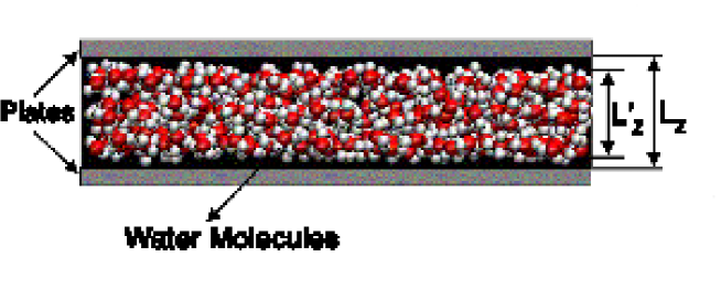
Figure 1: Schematic of the simulated system. Water molecules are confined between two smooth hydrophobic plates in an $xy$ plane, separated by $L_{z}=1.1$ nm. The figure also indicates $L_{z}^{\prime}$, the effective length of confinment of the water molecules.

In our simulation, water molecules are confined between two infinite smooth planar walls, as shown schematically in Fig. 1. The walls are located at $z=\pm 0.55$ nm, corresponding to a wall-wall separation of $1.1$ nm, which results in $\approx 2-3$ layers of water molecules. Periodic boundary conditions are used in the $x$ and $y$ directions, parallel to the walls.

The interactions between water molecules and the smooth walls are designed to mimic solid paraffin lee2 and are given by hansen

$$U\left(\Delta z\right)=4\epsilon_{\rm OW}\left[\left(\frac{\sigma_{\rm OW}}{\Delta z}\right)^{9}-\left(\frac{\sigma_{\rm OW}}{\Delta z}\right)^{3}\right].$$ (1)

Here $\Delta z$ is the distance from the oxygen atom of a water molecule to the wall, while $\epsilon_{\rm OW}=1.25$ kJ/mole and $\sigma_{\rm OW}=0.25$ nm are potential parameters. The same parameter values were used in previous confined water simulations lee1 ; lee2 .

We perform simulations for $56$ state points, corresponding to seven temperatures $T=220$, 230, 240, 250, 260, 280, and 300 K, and eight densities $\rho=0.80$, 0.88, 0.95, 1.02, 1.10, 1.17, 1.25, and 1.32 g/cm³ footnoteRealLz . The range of density values takes into account the fact that the water-wall interactions prevent water molecules from accessing a space near the walls. Our determination of $\rho$ is discussed in detail in the next section. The raw “geometric” densities used are $\rho=0.60$, 0.655, 0.709, 0.764, 0.818, 0.873, 0.927 and 0.981 g/cm³.

For each state point, we perform two independent simulations to improve the statistics. We control the temperature using the Berendsen thermostat with a time constant of $5$ ps berend and use a simulation time step of $1$ fs, just as in the bulk system masako . For long-range interactions we use a cutoff of $0.9$ nm jorgensen1 .

We calculate the lateral pressure $P_{\|}=(P_{xx}+P_{yy})/2$ using the virial expression for the $x$ and $y$-directions virial . We obtain the pressure along the transverse direction, $P_{\perp}$ by calculating the total force $F_{\rm wall}$ perpendicular to the wall meyer ,

$$P_{\perp}=\frac{F_{\rm wall}}{L_{x}L_{y}}=\frac{|\sum_{i=1}^{N}{\bf F}_{i,{\rm wall}}|}{L_{x}L_{y}}.$$ (2)

Here, ${\bf F}_{i,{\rm wall}}$ is the force produced by oxygen atom of water molecule $i$ on the wall. Hydrogen atoms do not interact with the wall. In agreement with the simulations of Ref. lee1 using the TIP4P model for water and the water-wall interaction given by Eq. (1), we find that the hydrogen atoms of the water molecules near a wall tend to face away from the wall, forming bonds with other molecules.

III Properties of TIP5P Confined Water

III.1 Transverse Density Profile

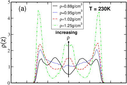
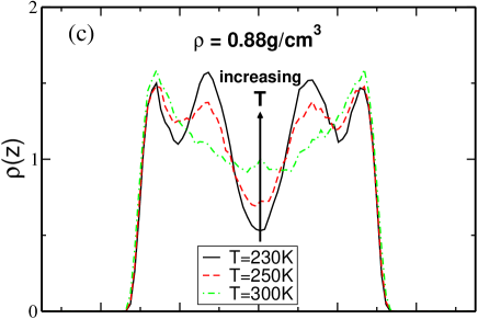
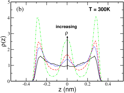
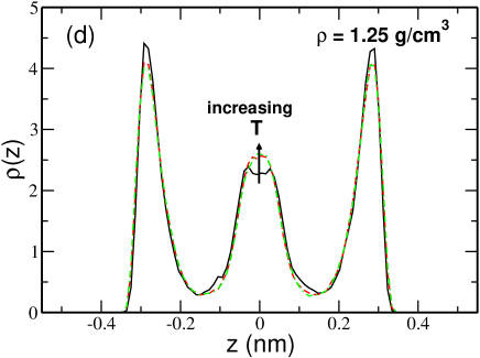
Figure 2: Density of water $\rho(z)$ along the confinement direction for different densities at constant temperatures (a) $T=230$ K and (b) $T=300$ K. (c) Density of water along the confinement direction for different temperatures at constant densities (c) $\rho=0.88$  g/cm³ and (d) $\rho=1.25$ g/cm³. See discussion in text.

One of the problems when dealing with liquids in a confined geometry is how to define the density in a consistent way. Using a geometric definition $\rho\equiv Nm/L_{x}L_{y}L_{z}$ (where $m$ is the water molecule mass) underestimates the effective density since the repulsive interactions with the walls prevent molecules from coming too close to the walls. Hence we want to quantify the effective distance $L^{\prime}_{z}$ perpendicular to the walls accessible to the water molecules (Fig. 1), and thus obtain a definition for $\rho$ which is more readily comparable with the density of a bulk system. To estimate $L^{\prime}_{z}$, we calculate the density profile $\rho(z)$ defined as the density of oxygen centers at $z$, shown in Fig. 2 for different temperatures and densities. In all cases studied, we observe that molecules cannot access the total available space between the walls, and that the accessible space along the transverse direction does not strongly depend on $T$ and $\rho$. Hence we estimate

$$L^{\prime}_{z}=L_{z}-\frac{\sigma_{\rm OW}+\sigma_{\rm OO}}{2}=0.819~{}{\rm nm}$$ (3)

independent of $T$ and $\rho$; this leads to the effective density

$$\rho\equiv{Nm\over L_{x}L_{y}L^{\prime}_{z}}.$$ (4)

Figure 2(a) shows the effect on $\rho(z)$ of changing $\rho$ at $T=230$ K. Since the typical oxygen-oxygen separation for nearest neighbor in bulk water is $0.28$ nm, for the effective wall separation $L^{\prime}_{z}=0.819$ nm one would expect that at most three water layers can be accommodated between the walls. At $\rho=1.02$ g/cm³ and $\rho=1.25$ g/cm³, $\rho(z)$ shows three clear maxima indicating the presence of a trilayer liquid. The two maxima next to the walls are the result of water-wall interaction. As density decreases below $\rho=1.02$ g/cm³, the central maximum becomes nearly uniform and, at density $\rho=0.95$ g/cm³, only the two maxima located next to the walls remain. This density corresponds to the least structured liquid. Upon further expansion, the structure of the liquid starts to increase since the bilayer splits into two sublayers for the lowest density $\rho=0.88$g/cm³. As we will see in the next section, $T=230$ K is below the temperature of maximum density ($T_{\rm MD}$). Hence the increase in the structure upon expansion corresponds to the anomalous decrease in entropy upon expansion found in bulk water below the $T_{\rm MD}$,

$$\left(\frac{\partial S}{\partial V}\right)_{T}=\left(\frac{\partial P}{\partial T}\right)_{V}=-\left(\frac{\partial V}{\partial T}\right)_{P}\left(\frac{\partial P}{\partial V}\right)_{T}\leq 0.$$ (5)

Figure 2(b) shows the effect on $\rho(z)$ of changing $\rho$ at higher $T$, $T=300$ K. The densities in Fig. 2(b) are the same as those shown in Fig. 2(a). Similar to findings at $T=230$ K, (i) the liquid at $T=300$ K and $\rho=1.25$ g/cm³ is characterized by a trilayer structure and (ii) reducing the density transforms the trilayer liquid into a bilayer liquid at $\rho=0.88$ g/cm³. However, comparison of Fig. 2(a) and r̃efrho-z(b) shows that, at the lowest $\rho$ studied, the layers of the bilayer structured liquid at $T=300$ K do not split into two sub-layers, as is the case of $T=230$ K since $T=300$ lies above the $T_{\rm MD}$. In fact, we find that at $T=230$ K the sublayers present at $\rho=0.88$ g/cm³ merge into a single layer at $\rho=0.95$ g/cm³, and the resulting $\rho(z)$ resembles that shown in Fig. 2(b) at $\rho=0.88$ g/cm³.

The effect of changing temperature at low density is shown in Fig. 2(c). As discussed above, at low density and low $T$ we observe a bilayer liquid where the two layers split into two sublayers. Increasing $T$ smoothes features of the density profile, namely (i) the splitting of the sublayers disappears, and (ii) the minimum of $\rho(z)$ at $z=0$ nm becomes less pronounced since increasing $T$ increases the entropy. While a bilayer $\rightarrow$ trilayer liquid crossover is found upon isothermal compression, isochoric heating does not have such an effect.

Figure 2(d) shows the effect of changing $T$ at the high density, $\rho=1.25$ g/cm³. At high $\rho$, the molecules are not able to displace perpendicular to the walls and the density profile is almost $T$ independent. Indeed, the liquid has a trilayer structure at all $T$ studied.

III.2 Low Temperature Phase Diagram

Next we test how confinement affects the location in the $P-T$ phase diagram of the LL phase transition line and the second critical point found in bulk water simulations using the TIP5P model masako ; paschek1 . To determine the phase behavior, we evaluate $P$ as a function of $\rho$. If there is a second LL phase critical point, then it should manifest itself in a van der Waals “loop” along isothermal paths at low $T$.

Unlike bulk liquid systems, one must be careful to interpret separately the results involving the lateral pressure $P_{\|}$ and those involving the transverse pressure $P_{\perp}$, since the thermodynamic averages of these quantities will usually be different. Phase separation will only be apparent in $P_{\|}$, since the separation of the plates is too small to allow for the existence of two distinct phases in the transverse direction. In Figs. 3(a) and 3(b), we show $P_{\perp}$ and the lateral pressure $P_{\|}$ as functions of density along all seven isotherms.

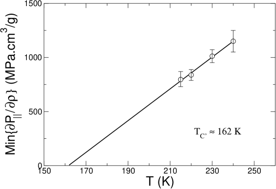
Figure 4: Minimum values of ($\partial P_{\|}/\partial\rho)_{T}$ as a function of temperature obtained from Fig. 3(d). The critical temperature $T_{C^{\prime}}$ of the critical point of the LL transition is crudely estimated by extrapolation.

Since there can be no phase separation in the transverse direction, $P_{\perp}$ is a monotonically increasing function of the density (Fig. 3(a)). $P_{\|}$ is also a monotonic increasing function of $\rho$, but as $T$ decreases, the isotherms of $P_{\|}$ become “flatter” in the region near $\rho\approx 0.95$ g/cm³ (Fig. 3(b)). The presence of this region is consistent with the possible existence of a van der Waals loop at lower $T$ and, therefore, is consistent with the possible existence of a LL phase transition line ending at a second critical point at a value of $T$ lower than 220 K, the lowest simulated temperature. At 220 K no phase separation occurs, consistent with the simulations of bulk water where the same TIP5P potential gives a second critical point with $T_{C^{\prime}}=217\pm 3$ K masako . While we are unable to simulate the temperatures below $T_{C^{\prime}}$ of the bulk system, comparison of the lowest $T$ isotherm with that of Ref. masako ; paschek1 suggests that we will need to go well below the bulk $T_{C^{\prime}}$ to see phase separation. Thus our results suggest that the presence of hydrophobic walls shifts a possible second critical point to lower $T$. Along an isothermal path, the critical point can be located by the point where the slope $(\partial P/\partial\rho)_{T}$ and curvature $(\partial^{2}P/\partial\rho^{2})_{T}$ simultaneously equal zero. We can estimate this point by plotting the values of the minimum slopes along each isotherm and extrapolating the slopes to find the $T$ at which the slope is zero. This estimate yields critical temperature $T_{C^{\prime}}\approx 162\pm 20$ K (Fig. 4).

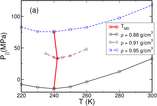
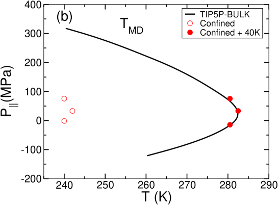
Figure 5: A comparison of $T_{\rm MD}$ line for bulk and confined water. (a) Isochores corresponding to the densities $\rho=0.88$g/cm³, $\rho=0.91$g/cm³ and $\rho=0.95$g/cm³ which have a minimum. The locus of the points where $(\partial P_{\|}/\partial T)_{V}=0$ denotes the $T_{\rm MD}$ (shown as asterisk). (b) If the $T_{\rm MD}$ for confined water (open circles) were shifted by $40$ K, it would overlap the $T_{\rm MD}$ for bulk water (filled circles).

Figures 3(c) and 3(d) show the $T$-dependence of $P_{\perp}$ and $P_{\|}$ for different densities. $P_{\perp}(T)$ is a monotonic function of $T$ for all $\rho$. Similar behavior is observed for $P_{\|}(T)$ at large $\rho$. However, for $0.88$ g/cm³ $\leq\rho\leq 1.17$ g/cm³, the isochores in the $P_{\|}-T$ plane display minima, indicating the presence of a $T_{\rm MD}$ line, defined as the locus of points where $(\partial P/\partial T)_{V}=0$ hansen . For $T<T_{\rm MD}$, water confined between hydrophobic walls is anomalous, i.e., it becomes less dense upon cooling. A $T_{\rm MD}$ line has also been found in TIP5P bulk water simulations masako . Comparison of Fig. 3(c) and Fig. 2(a) of Ref. masako shows that the $T_{\rm MD}$ locus in confined water shifts to lower $T$. We also plot the $T_{\rm MD}$ for bulk water (from Ref. masako ) and confined water in Fig. 5. A $+40$ K temperature shift in the $T_{\rm MD}$ of confined water overlaps these loci. Thus the effect of the hydrophobic walls in our system seems to be to shift the $P-T$ phase diagram by $\Delta T\approx-40\pm 5$ K with respect to bulk water. This is consistent with the second critical point shifting to lower $T$.

Figure 6 shows the calculated potential energy for the lowest simulated temperature $T=220$ K. We note two minima for the densities around $\rho=0.88$g/cm³ and $\rho=1.39$g/cm³ respectively. Since the free energy $F$ is given by

$$F=K+U-TS,$$ (6)

where $K$, $U$, and $S$ are the kinetic energy, potential energy and entropy respectively, at small $T$ an extremum in $U$ suggests an extremum in $F$. Hence the emergence of two minima at small $T$ further supports the possibility of two stable liquids at low and high densities respectively.

IV Static Structure

IV.1 Radial Distribution Function

In Sec. II we studied the structure of water along the direction perpendicular to the walls. To aid in comparing the structural properties with those of bulk water, we next focus on the lateral oxygen-oxygen radial distribution function (RDF) defined by

$$g_{\|}(r)\equiv\frac{1}{\rho^{2}V}\sum_{i\neq j}\delta(r-r_{ij})\left[\theta\left(|z_{i}-z_{j}|+\frac{\delta z}{2}\right)-\theta\left(|z_{i}-z_{j}|-\frac{\delta z}{2}\right)\right].$$ (7)

Here $V$ is the volume, $r_{ij}$ is the distance parallel to the walls between molecules $i$ and $j$, $z_{i}$ is the $z$-coordinate of the oxygen atom of molecule $i$, and $\delta(x)$ is the Dirac delta function. The Heaviside functions, $\theta(x)$, restrict the sum to a pair of oxygen atoms of molecules located in the same slab of thickness $\delta z=0.1$ nm. The physical interpretation of $g_{\|}(r)$ is that $g_{\|}(r)2\pi rdr\delta z$ is proportional to the probability of finding an oxygen atom in a slab of thickness $\delta z$ at a distance $r$ parallel to the walls from a randomly chosen oxygen atom. In a bulk liquid, this would be identical to $g(r)$, the standard RDF.

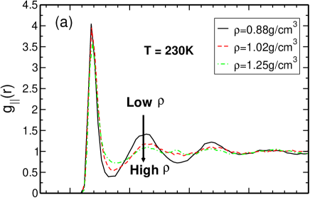
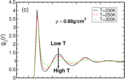
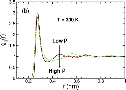
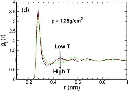
Figure 7: Lateral oxygen-oxygen radial distribution function $g_{||}(r)$ for different densities at a constant temperature (a) $T$ = $230K$ and (b) $T=300$ K; $g_{||}(r)$ for different temperatures at a constant density (c) $\rho$ = $0.88$ g/cm³ and (d) $\rho=1.25$ g/cm³.

Figure 7(a) shows the effect on $g_{\|}(r)$ of increasing $\rho$ at low $T$. At low $\rho$, the bilayer liquid is characterized by a RDF that resembles the RDF of bulk water at $\rho=0.99$ g/cm³ finneyPRL , with maxima at $r\approx 0.28$, 0.45, and 0.67 nm. The well-defined maxima and minima in both $\rho(z)$ (Fig. 2(a)) and $g_{\|}(r)$ (Fig. 7(a)) indicate that at low-$T$ and low-$\rho$ the liquid is highly structured, with a structure parallel to the walls similar to corresponding bulk liquid water at low density soperRicci . As $\rho$ increases, the liquid becomes less structured as indicated by the decreasing height of the second and third peaks of $g_{\|}(r)$, and by the disappearance of the sublayers in $\rho(z)$ (Fig. 2(a)). A comparison of $g_{\|}(r)$ at $\rho=1.25$ g/cm³ with the $g(r)$ for bulk water at high density from Ref. soperRicci shows that the distributions are very different. However, we find that if we calculate $g_{\|}(r)$ for only $-0.17$ nm $\leq z\leq 0.17$ nm (which corresponds to the location of the central layer), then $g_{\|}(r)$ at low-$\rho$ and high-$\rho$ resemble $g(r)$ for bulk water at both low and high densities respectively. Thus the evolution of the structure parallel to the walls of the central layer mimics the structural changes when going from low-density bulk water to high-density bulk water.

The effect of increasing the density at $T=300$ K is shown in Fig. 7(b). The main effect of compression is to “redistribute” the molecules parallel to the walls. At $\rho=0.88$ g/cm³, $g_{\|}(r)$ is similar to the distribution shown in Fig. 7(a) at the same density, which resembles $g(r)$ for low-density bulk water. However, the maxima and minima in $g_{\|}(r)$ are less pronounced at $T=300$ K. At intermediate $\rho$, $g_{\|}(r)$ becomes very close to $1$ for $r>0.45$ nm. As density increases up to $\rho=1.25$ g/cm³, a weak peak appears at $r\approx 0.9$ nm and a maximum occurs at $0.55$ nm. Furthermore, the first maximum of $g_{\|}(r)$ becomes wider and the first minimum shift towards $r\approx 0.4$ nm. The resulting $g_{\|}(r)$ at high $\rho$ and high $T$ has many features of $g(r)$ for bulk water obtained experimentally at $T=268$ K soperRicci . For example, the oxygen-oxygen $g(r)$ in Ref. soperRicci shows a weak peak at $r\approx 0.9$ nm, a clear maximum at $0.61$ nm, and the first minimum is located at $r\approx 0.41$ nm. Furthermore, a shoulder in the first maximum of $g(r)$ develops at high density which is consistent with the increase of the width of the first peak of $g_{\|}(r)$ in Fig. 7(b) as $\rho$ increases.

To complete the comparison of the structure of confined water with the structure of bulk water, we also evaluate the $T$-dependence of $g_{\|}(r)$. In Fig. 7(c), we show $g_{\|}(r)$ for various $T$ at $\rho=0.88$ g/cm³. The effects of increasing $T$ at low $\rho$ are similar to those observed in Fig. 7(a) when increasing $\rho$ at low $T$. More specifically, the minima and maxima of $g_{\|}(r)$ become less pronounced as $T$ increases and $g_{\|}(r)$ becomes flatter for $r>0.5$ nm. We note that similar changes are also found in $\rho(z)$ when (i) increasing $T$ at low $\rho$ (Fig. 2(a)) and (ii) increasing $\rho$ at low $T$ (Fig. 2(c)).

Figure 7(d) shows the effect of $T$ on $g_{\|}(r)$ when the density is fixed at $\rho=1.25$ g/cm³. The effects of increasing $T$ at high $\rho$ (Fig. 7(d)) are similar to the effects of increasing $\rho$ at a high $T$ (Fig. 7(b)). More specifically, the first minimum of $g_{\|}(r)$ shifts to a larger $r$ and becomes less pronounced, while the second and third peaks located at $0.45$ nm and $0.7$ nm, respectively, merge and form an intermediate peak at $r=0.55$ nm. This suggests that as $\rho$ increases at high $T$, the preferred distance between second neighbors increases (parallel to the walls) and local tetrahedral order decreases. The emergence of a peak at $0.55$ nm on heating at 1.25 g/cm³ is in contrast to the behavior of bulk water, where the disappearance of the peaks at 0.45 and 0.7 nm gives rise to nearly featureless behavior of $g(r)$ beyond the first peak (see, e.g., Ref. sslsss ). Hence at high $T$, confinement gives rise to structure that would not be present in bulk systems, presumably because molecules orient relative to the walls. It is interesting to note that, as shown in Sec. 2, there is almost no change in $\rho(z)$ with $T$, indicating that the rearrangement of the molecules parallel to the walls has no effect, on average, on the organization of molecules perpendicular to the walls.

IV.2 Static Structure Factor

Next we calculate the lateral static structure factor $S_{\|}(q)$, defined as the Fourier transform of the lateral radial distribution function $g_{\|}(r)$,

$$S_{\|}\left(q\right)=\frac{1}{N}\sum_{i,j}\left<e^{i\vec{\bf q}.(\vec{\bf r_{i}}-{\bf\vec{r_{j}}})}\right>,$$ (8)

where the $q$-vector is the inverse space vector in the $xy$ plane and $r$ is the projection of the position vector on the $xy$ plane. The structure factor will be particularly useful for comparison with the crystal structure in Sec. VI, where distinct Bragg peaks in $S_{\|}\left(q\right)$ appear.

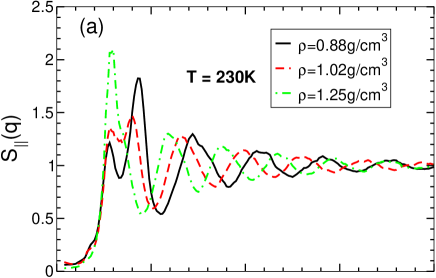
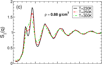
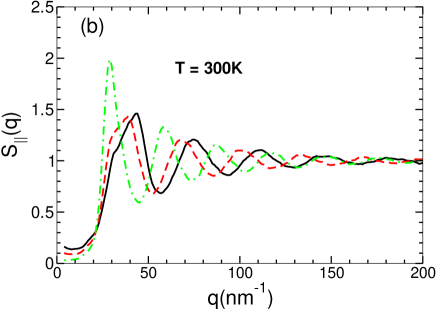
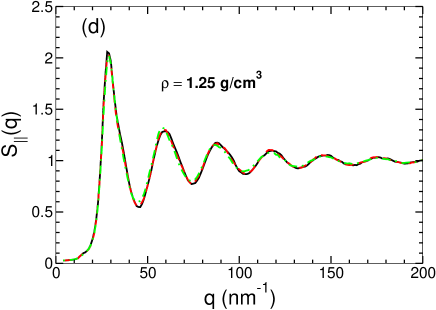
Figure 8: Lateral structure factor $S_{\|}(q)$ for different densities at a constant temperature (a) $T=230$ K and (b) $T=300$ K; $S_{\|}(q)$ for different temperatures a constant density (c) $\rho=0.88$ g/cm³ and (d) $\rho=1.25$ g/cm³.

Figures 8(a) and 8(b) show the effect of density on the lateral structure factor $S_{\|}(q)$ for $T=230$ K and $T=300$ K. The structure factor of low-density and low-temperature confined water is similar to bulk water. The presence of a “pre-peak” in $S_{\|}\left(q\right)$ at low $\rho$ can be attributed to the existence of pronounced tetrahedral order in the low-temperature liquid. At high $\rho$ or high $T$, this feature is reduced, as the molecular order becomes less tetrahedral and core repulsion dominates. This behavior is similar to bulk water, but with a shift to lower densities. We show the evolution of $S_{\|}(q)$ as a function of $T$ for two different densities $\rho=0.88$ g/cm³ and $\rho=1.25$ g/cm³ in Figs. 8(c) and 8(d). The structure of low-temperature water for $\rho=0.88$ g/cm³ is similar to low-density water. When the temperature is increased, the repulsive region of the potential begins to dominate and tetrahedrality is reduced. The first two peaks in the structure factor merge to form a single peak (Fig. 8(c)). However, at high density $\rho=1.25$ g/cm³, a change is temperature does not change the structure factor significantly (Fig. 8(d)). Similar behavior is seen in bulk water francis .

V Dynamics

Thus far, we have seen that if a LL transition exists for confined water, it is shifted to lower $T$ than for bulk water, and that the tetrahedral order that gives rise to this behavior is also suppressed. Hence it is natural to consider whether the dynamic properties of confined water exhibit the same temperature shift found for the thermodynamic properties relative to bulk water. For example, how is the maximum in diffusivity under pressure shifted under confinement? To compare with the bulk system, we calculate the lateral mean square displacement (MSD). We can evaluate the diffusion coefficient $D$ from the asymptotic behavior of the lateral MSD using the Einstein relation

$$\langle r_{\|}^{2}\rangle=2dDt,$$ (9)

where $\langle r_{\|}^{2}\rangle$ is the mean square displacement parallel to the walls over a given time interval $t$, and $d$ is the system dimension benedek . Since we calculate the diffusion only in the lateral directions, $d=2$.

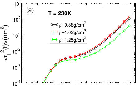
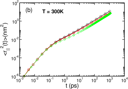
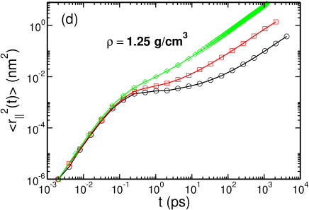
Figure 9: Lateral mean square displacement $\langle r_{\|}^{2}(t)\rangle$ for different densities at constant temperatures (a) $T=230$ K and (b) $T=300$ K. $\langle r_{\|}^{2}(t)\rangle$ for different temperatures at constant densities (c) $\rho=0.88$ g/cm³ and (d) $\rho=1.25$ g/cm³.

Figures 9(a) and 9(b) show the dependence of the lateral MSD on $\rho$ at fixed $T=230K$ and $T=300K$. We also plot the dependence of the lateral MSD on $T$ for two different temperatures in Figs. 9(c) and 9(d), using a log-log scale to emphasize the different mechanisms seen on different time scales:

• An initial ballistic motion, where the lateral MSD is a quadratic function of time, $\langle r_{\|}^{2}(t)\rangle\sim t^{2}$.

• An intermediate “flattening” of the lateral MSD, due to the transient caging of molecules by their hydrogen bonded neighbors. This effect is most noticeable at the lowest $T$ studied, and does not occur at high $T$.

• Long time scales on which particles diffuse randomly, and so $\langle r_{\|}^{2}(t)\rangle\sim t$.

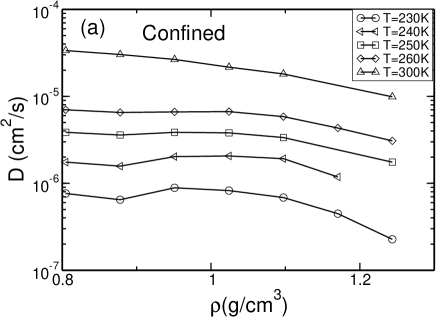
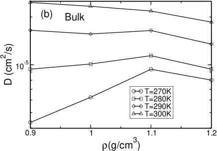
Figure 10: Diffusion constant $D$ as a function of density for various temperatures in (a) confined water and (b) bulk water. Confined water shows diffusion anomalies at lower temperatures than in bulk water. The first diffusion anomaly (the increase of diffusion with increase in density) in the confined system begins to appear when the temperature drops to $T\approx 250$ K, which is $\approx 40$ K lower than in bulk water (which displays diffusion anomalies at $T\approx 290K$).

To determine whether there is an anomaly in the density dependence of $D$, we plot $D$ along isotherms, in Fig. 10(a) for confined water and in Fig. 10(b) for bulk water. For $T\lesssim 250$ K, we find that $D$ has a maximum at $\rho\approx 1.05$ g/cm³. In bulk water, a similar behavior is found, but at $T\approx 290$ K, $40$ K higher than the confined system. Moreover, this shift in a dynamic anomaly is consistent with the shift of thermodynamic anomalies. Qualitatively, the maximum in $D$ can be understood as a competition between weakening or breaking of hydrogen bonds under pressure sns (which increases $D$) and increased packing (which reduces $D$).

We next study the effect of confinement on the rotational motion of water molecules. The rotational motion was analyzed by calculating the rotational autocorrelation time for all the state points and are compared with the rotational autocorrelation time for bulk water for few state points. The rotational autocorrelation function $C_{1}(t)$ is defined as

$$C_{1}(t)\equiv\frac{1}{N}\left\langle\sum_{i=1}^{N}{\vec{e}_{i}(t).\vec{e}_{i}(0)}\right\rangle,$$ (10)

where $\vec{e}_{i}(t)$ is the unit dipole vector of molecule $i$ at time $t$. For large times, $C_{1}(t)$ can be fit with a stretched exponential function

$$C_{1}(t)=Ae^{(-t/\tau)^{\beta}}$$ (11)

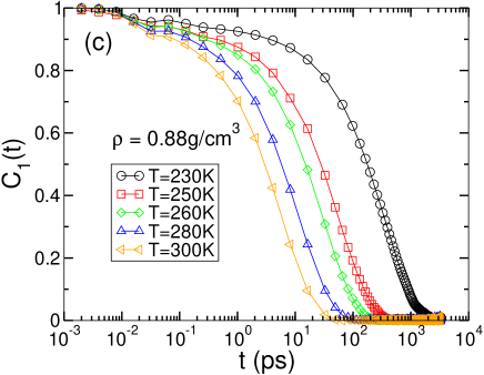
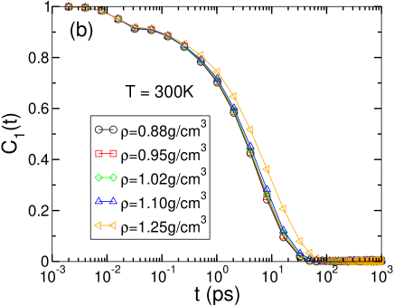
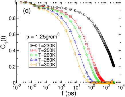
Figure 11: Dipole-dipole autocorrelation function $C_{1}(t)$ for different densities at constant temperature (a) $T=230$ K and (b) $T=300$ K. Also shown is $C_{1}(t)$ for different temperatures at constant density (c) $\rho=0.88$ g/cm³ and (d) $\rho=1.25$ g/cm³.

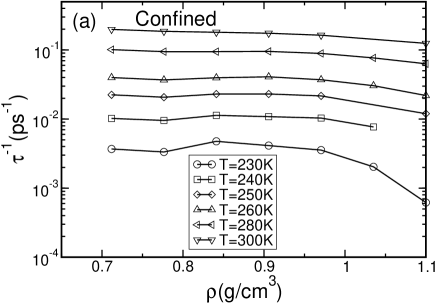
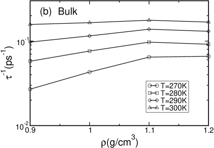
Figure 12: Inverse orientational autocorrelation time as a function of density for (a) confined water and (b) bulk water. Inverse autocorrelation time for confined water follows a similar behavior as bulk water, but temperature shifted by $\approx 40$ K to lower $T$.

where $A$, $\beta\leq 1$ are constants and $\tau=\tau(\rho,T)$ is the orientational autocorrelation time, which depends on both density and temperature. In Fig. 11, we show $C_{1}(t)$ for different temperatures and densities. Figure 12(a) shows the inverse of the orientational autocorrelation time which is proportional to the rotational diffusion. For a comparison with the bulk water rotational diffusion, $\tau^{-1}$ is also shown in Fig. 12(b). Both the translational diffusion constant [Fig. 10(a)] and the inverse of the orientational autocorrelation time [Fig. 12(a)] show similar behavior. Similar results have been found for bulk water with the SPC/E potential netz . For low temperature, the maxima occur at the same density for $D$ and $\tau^{-1}$. However at high temperatures ($T\geq 260K$), where the $D$ is a monotonically decreasing function of density, $\tau^{-1}$ has a maximum and a minimum similar to its bulk counterpart [Fig. 12(b)].

VI Crystallization of TIP5P Confined Water

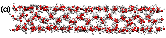
Figure 13: Trilayer ice with $L_{z}=1.1$ nm and $\rho=1.32$ g/cm³ formed when the system is cooled from $T=320$ K to $T=260$ K. (a) A lateral snapshot. (b) Lateral structure factor.

Bulk TIP5P water crystallizes within the simulation time at higher densities and, for a given density, the crystallization time has a minimum at $T=240$ K masako . We next investigate whether crystallization occurs in confinement, and whether the structure differs due to the surface effects. It has been found experimentally that water confined in hydrophobic carbon nanopores does not crystallize, even at very low temperatures bellisent . However, the crystallization of confined water is seen in some simulations zangi1 ; koga1 . We find that our system crystallizes to what appears to be a trilayered ice structure at high density and that the resultant ice has a density $\rho=1.32$ g/cm³. A similar crystallization appears in simulations when an electric field is applied in a lateral direction zangi2 . The surface in this kind of simulation exhibits the embedded crystal structure of silica, where the oxygen and silicon atoms are arranged in out-of-registry order. This suggests that the crystalline form we find in confinement does not depend on the morphology of the surface. We show the structure of the ice and the static lateral structure factor in Fig. 13.

To investigate whether confined water crystallizes in the same crystalline form when the separation between the plates is different, we repeat our simulation for a plate separation of $0.7$ nm, and again the system crystallizes at $T=260$ K. The system crystallizes into a monolayer ice, also seen in simulations in Ref. zangi1 . The ice structure and its lateral static structure factor are shown in Fig. 14. The density of monolayer ice is $\rho=0.93$ g/cm³ . We list the temperature, pressure, and potential energy for these crystals in Table I.

VII Conclusions

We have systematically investigated the effect of confinement on TIP5P water between two parallel smooth hydrophobic plates, separated by $1.10$ nm. We found that the overall phase-diagram is shifted to lower temperature and lower density compared to bulk TIP5P water by $\Delta T\approx-40$K. The shift to lower temperature compared to the bulk water can be understood qualitatively. Since the confinement walls do not form any hydrogen bonds with water molecules the average number of hydrogen bonds per molecule in confined system is smaller than in bulk water. This is analogous to having bulk water at high temperatures.

We do not see a LL phase transition for the state points we have been able to simulate, but we do see a pronounced inflection in the $P-\rho$ isotherms (Fig. 3), which is consistent with a LL phase transition at lower $T$. Since the phase diagram is shifted $\approx 40$ K lower in temperature, our results are consistent with the possibility that there indeed is a LL transition at a temperature too low to simulate. This shift of thermodynamics qualitatively agrees with the theoretical predictions of Ref. truskett . The structure of confined water is similar to the structure bulk water at a lower density, and shows a similar evolution of the structure with changes in density and temperature. At a given temperature, as the density increases, water changes from a bilayer liquid (at low density) to a trilayer liquid (at high density). We find that the confinement affects the translational diffusion as well as the rotational motion of water molecules. The rotational diffusion anomaly precedes the translational diffusion anomaly, just as occurs for bulk water.

We were able to crystallize water for a few state points. It crystallizes spontaneously to a trilayer ice at T=260K. Monolayer ice was formed when the separation between the plates was decreased to $0.7$ nm. The crystalline structures are different from the polymorphs of bulk water, and should be relevant for confined water.

VIII Acknowledgments

We thank C.A. Angell, E. La Nave, and F. Sciortino for discussions, NSF grants CHE-0096892, CHE-0404699, and DMR-0427239 for support. We also thank the Boston University Computational Center, Wesleyan University, and Yeshiva University for supporting computational facilities.

Table 1: Thermodynamic properties of the crystals formed at $T=260K$

Plate Separation (nm)	Pressure (MPa)	Potential Energy (kJ/mol)
0.7	–90.30	–39.86
1.1	652.89	–44.08

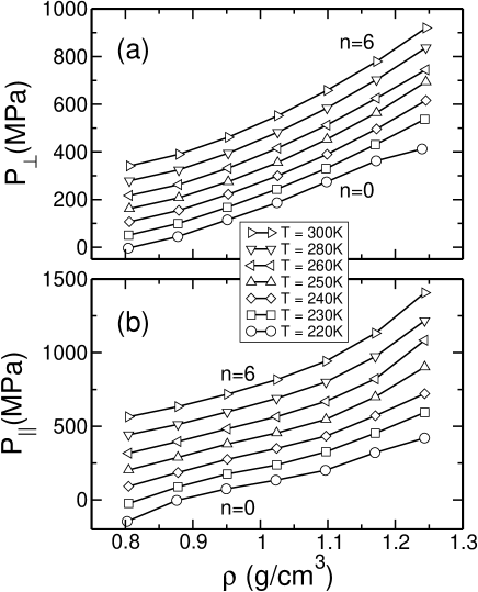
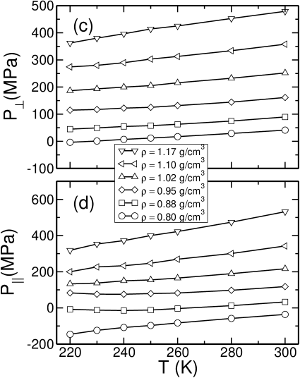
Figure 3: (a) Transverse pressure $P_{\perp}$ (perpendicular to the walls) and (b) lateral pressure $P_{\|}$ (parallel to the walls) as functions of density $\rho$ for all simulated $T$. For clarity, each curve is shifted by $n\times 50$MPa for $P_{\perp}$ for and $n\times 100$MPa for $P_{\|}$. While $P_{\perp}$ shows no infection for all $T$, $P_{\|}$ starts to flatten at $\rho\approx 0.87$ g/cm³ for the lowest $T$ presented. This is consistent with the possibility of a second critical point at lower than $T=220$ K. (c) $P_{\perp}$ and (d) $P_{\|}$ as a function of temperature for different densities. Only $P_{\|}$ displays minima, indicating the presence of a $T_{\rm MD}$.

Figure 6: Potential energy as a function of $\rho$ for the lowest temperature we simulate, indicating the possibility of two stable liquid states at $\rho=0.88$g/cm³ and $\rho=1.39$g/cm³. The two minima are indicated by vertical arrows.

Figure 14: Monolayer ice with $L_{z}=0.7$ nm and $\rho=0.93$ g/cm³ spontaneously formed at $T=260$ K. (a) A lateral snapshot and (b) top view. (c) Lateral structure factor.

References

- (1) C. A. Angell, Ann. Rev. Chem. 34, 593 (1983).
- (2) P. G. Debenedetti, J. Phys. Cond. Mat. 15, R1669 (2003).
- (3) P. G. Debenedetti and H. E. Stanley, Physics Today 56 (6), 40 (2003).
- (4) V. Brazhkin. S. V. Buldyrev, V. N. Ryzhov, and H. E. Stanley, eds., New Kinds of Phase Transitions: Transformations in Disordered Substances (Kluwer, Dordrecht, 2002).
- (5) R. Zangi, J. Phys. Cond. Mat. 16, S5371 (2004).
- (6) I. D. Gelb, K. E. Gubins, R. Radhakrishnan, and M. S. Bartkoviak, Rep. Prog. Phys. 61, 1573 (1999).
- (7) K. Lum, D. Chandler, and J. D. Weeks, J. Phys. Chem. B 103, 4590 (1999).
- (8) Simulations show that the folding transition of a protein occurs at the same time as the formation of hydrophobic protein cores in water. See R. Zhou, B. J. Berne, and R. Germain, Proc. Nat. Acad. Sci. 98, 14931 (2001); M. Tarek and D. J. Tobias, Phys. Rev. Lett. 89, 275501 (2002).
- (9) P. Scheidler, W. Kob, and K. Binder, Europhys. Lett. 59, 701 (2002).
- (10) M.-C. Bellissent-Funel, R. Sridi-Dorbez, and L. Bosio, J. Chem. Phys. 104, 10023 (1996).
- (11) S.-H. Chen, P. Gallo, and M.-C. Bellissent-Funel, Can. J. Phys. 73, 703 (1995).
- (12) S.-H. Chen and M.-C. Bellissent-Funel, in Hydrogen Bond Networks, edited by M.-C. Bellissent-Funel and J. C. Dore, NATO ASI Ser. C: Math. Phys. Sci., Vol. 435 (Kluwer Academic, Dordrecht, 1994), p. 337.
- (13) P. Gallo and M. Rovere, J. Phys. Condensed Matter 15, 1521 (2002).
- (14) E. Spohr, C. Hartnig, P. Gallo, and M. Rovere, J. Mol. Liq. 80, 165 (1999).
- (15) P. Gallo, M. A. Ricci, M. Rovere, C. Hartnig, and E. Spohr, Europhys. Lett. 49, 183 (2000).
- (16) C. Hartnig, W. Witschel, E. Spohr, P. Gallo, M. A. Ricci, and M. Rovere, J. Mol. Liq. (2000, in press).
- (17) P. Gallo, M. Rovere, M. A. Ricci, C. Hartnig, and E. Spohr, Philos. Mag. B 79, 1923 (1999).
- (18) P. Gallo, Phys. Chem. Chem. Phys. 2, 1607 (2000).
- (19) P. H. Poole, F. Sciortino, U. Essmann, and H. E. Stanley, Nature 360, 324 (1992).
- (20) O. Mishima and H. E. Stanley, Nature 396, 329 (1998).
- (21) P. H. Poole, F. Sciortino, T. Grande, H. E. Stanley, and C. A. Angell, Phys. Rev. Lett. 73, 1632 (1994).
- (22) F. Sciortino, P. H. Poole, U. Essmann, and H. E. Stanley, Phys. Rev. E 55, 727 (1997).
- (23) H. E. Stanley, L. Cruz, S. T. Harrington, P. H. Poole, S. Sastry, F. Sciortino, F. W. Starr, and R. Zhang, Physica A 236, 19 (1997).
- (24) F. Sciortino, E. La Nave, and P. Tartaglia, Phys. Rev. Lett. 91, 155701 (2003).
- (25) M. Yamada, S. Mossa, H. E. Stanley, and F. Sciortino, Phys. Rev. Lett. 88, 195701 (2002).
- (26) S. Harrington, P. H. Poole, F. Sciortino, and H. E. Stanley, J. Chem. Phys. 107, 7443 (1997).
- (27) O. Mishima and H. E. Stanley, Nature 392, 164 (1998).
- (28) A. Faraone, L. Liu, C.-Y. Mou, C.-W. Yen and S.-H. Chen, J. Chem. Phys. 121, 10843 (2004).
- (29) S.-H. Chen et al., private communication.
- (30) S. Engemann, H. Reichert, H. Dosch, J. Bilgram, V. Honkimaki, and A. Snigirev, Phys. Rev. Lett. 92, 205701 (2004).
- (31) E. A. Jagla, Phys. Rev. E 58, 1478 (1998); E. A. Jagla, J. Chem. Phys. 110, 451 (1999); E. A. Jagla, J. Chem. Phys. 111, 8980 (1999).
- (32) S. V. Buldyrev, G. Franzese, N. Giovambattista, G. Malescio, M. R. Sadr-Lahijany, A. Scala, A. Skibinsky, H. E. Stanley, Physica A 304, 23 (2002).
- (33) G. Franzese, G. Malescio, A. Skibinsky, S. V. Buldyrev and H. E. Stanley, Nature 409, 692 (2001).
- (34) G. Franzese, G. Malescio, A. Skibinsky, S. V. Buldyrev and H. E. Stanley, Phys. Rev. E 66, 051206 (2002).
- (35) P. Kumar, S. V. Buldyrev, F. Scioritno, E. Zaccarelli, H. E. Stanley, Phys. Rev. E (in press) and cond-mat/0411274 (2004).
- (36) M. W. Mahoney and W. L. Jorgensen, J. Chem. Phys. 112, 8190 (2000).
- (37) M. W. Mahoney and W. L. Jorgensen, J. Chem. Phys. 114, 363 (2001).
- (38) D. Paschek, arXiv:cond-mat/0411724.
- (39) M. Meyer and H. E. Stanley, J. Phys. Chem. B 103, 9728 (1999).
- (40) W. L. Jorgensen, J. Chandrasekhar, J. Madura, R. W. Impey and M. Klein, J. Chem. Phys. 79, 926 (1983).
- (41) H. Tanaka, Nature, 380, 6572 (1996).
- (42) H. Tanaka, J. Chem. Phys. 105, 5099 (1996).
- (43) K. Koga, H. Tanaka, and X. C. Zeng, Nature, 408, 564(2000).
- (44) K. Koga and H. Tanaka, J. Chem. Phys. 122, 104711 (2005).
- (45) T. M. Truskett and P. G. Debenedetti, J. Chem. Phys. 114, 2401 (2001).
- (46) K. Koga, X. C. Zeng, and H. Tanaka, Phys. Rev. Lett. 79, 5262 (1997).
- (47) R. Zangi and A. E. Mark, Phys. Rev. Lett. 91, 0255502 (2003).
- (48) R. Zangi and A. E. Mark, J. Chem. Phys. 120, 7123 (2004).
- (49) J. Slovak, K. Koga, H. Tanaka, and X.C. Zeng, Phys. Rev. E 605833 (1999).
- (50) F. H. Stillinger and A. Rahman, J. Chem. Phys. 60, 1545 (1974).
- (51) J. M. Sorenson, G. Hura, R. M. Glaeser, and T. Head-Gordon, J. Chem. Phys. 113, 9149 (2000).
- (52) Matsumoto M, Saito S, and Ohmine I., Nature, 416 6879(2002).
- (53) L. A. Baez and P. Clancy, J. Chem. Phys. 103, 9744 (1995).
- (54) C. Y. Lee, J. A. McCammon, and P. J. Rossky, J. Chem. Phys. 80, 4448 (1984).
- (55) J. P. Hansen and I. R. McDonald, Theory of Simple Liquids, (Academic Press, London, 1996).
- (56) S. H. Lee and P. J. Rossky, J. Chem. Phys. 100, 3334 (1994).
- (57) We note the the accessible volume to the water molecules is not given by the total geometrical volume between the walls, . Instead, the accessible volume is given by where due to the repulsive wall-water interactions for short distances. The calculation of is explained in Sec. III.1.
- (58) H. J. C. Berendsen, J. P. M. Postma, W. F. van Gunsteren, A. DiNola and J. R. Haak, J. Chem. Phys. 81, 3684 (1984).
- (59) M. P. Allen and D. J. Tildesley, Computer Simulation of Liquids (Oxford University Press, 1997).
- (60) J. L. Finney, A. Hallbrucker, I. Kohl, A.K. Soper, and D.T. Bowron, Phys. Rev. Lett. 88, 225503 (2002).
- (61) A.K. Soper and M.A. Ricci, Phys. Rev. Lett. 84, 2881 (2000).
- (62) F. W. Starr, S. Sastry, E. La Nave, A. Scala, H. E. Stanley and F. Sciortino, Phys. Rev. E 63, 041201 (2001).
- (63) F. W. Starr, S. T. Harrington, F. Sciortino, and H. E. Stanley, Phys. Rev. Lett. 82, 3629 (1999); F. W. Starr, F. Sciortino, and H. E. Stanley, Phys. Rev. E 60, 1084 (1999).
- (64) G. Benedek and F. Villars, Physics with illustrative examples from medicine and biology (Addison Wesley, Reading, 1975)
- (65) F. W. Starr, J. K. Nielsen, and H. E. Stanley, Phys. Rev. Lett. 82, 2294 (1999); Phys. Rev. E 62 579 (2000).
- (66) P. A. Netz, F. Starr, M. C. Barbosa, H. E. Stanley, J. Mol. Liq. 101, 159 (2002); P. A. Netz, F. W. Starr, H. E. Stanley, and M. C. Barbosa, J. Chem. Phys. 115, 344–348 (2001).