Coulomb Interactions and Ferromagnetism in Pure and Doped Graphene

Abstract

We study the presence of ferromagnetism in the phase diagram of the two-dimensional honeycomb lattice close to half-filling (graphene) as a function of the strength of the Coulomb interaction and doping. We show that exchange interactions between Dirac fermions can stabilize a ferromagnetic phase at low doping when the coupling is sufficiently large. In clean systems the zero temperature phase diagram shows both first order and second order transition lines and two distinct ferromagnetic phases: one phase with only one type of carriers (either electrons or holes) and another with two types of carriers (electrons and holes). Using the coherent potential approximation we argue that disorder further stabilizes the ferromagnetic phase. This work should estimulate Monte Carlo calculations in graphene dealing with the long-range nature of the Coulomb potencial.

I Introduction

The ferromagnetic instability due to the exchange interaction in a three dimensional (3D) electron gas attracted attention since the early days of quantum mechanics Bloch (1929) and has been studied in great detail Iwamoto and Sawada (1962); Misawa (1965). Recent Monte Carlo calculations Ceperley (1978); Ceperley and Alder (1980) have confirmed the presence of ferromagnetism in the phase diagram of the 3D electron gas at low doping. Similar studies have also suggested the existence of a ferromagnetic phase in the diluted two dimensional (2D) electron gas Attaccalite et al. (2002) with a first order transition from a paramagnetic phase to a ferromagnetic phase with full polarization. As the electron density is reduced, electron-electron interactions become stronger and dynamical screening disappear. At the extreme limit of zero density the electron gas should crystalize into a Wigner solid where the electrons feel the unscreened Coulomb interaction. The elusive ferromagnetic phase of the electron gas lurks between the Wigner crystal and the Fermi liquid state that exists at higher doping when electron-electron interactions are fully screened Attaccalite et al. (2002); Ceperley (1999).

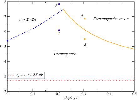
Figure 1: Zero temperature phase diagram of a clean graphene plane as a function of the coupling constant $g$, eq. (1), and doping away from half-filling. The dashed line corresponds to a first order, and the continuous line a second order phase transition between the paramagnetic and ferromagnetic phases. The dotted curve corresponds to the value of $g$ with $\epsilon_{0}=1$ and a Dirac-Fermi velocity of $\hbar v_{\rm F}=5.7$ eV $\AA$, as defined by Eq.(1). The points labeled 1-4 in the figure are discussed ahead in the text in connection with Fig. 3.

In recent years, the experimental search for the ferromagnetic phase of the diluted electron gas has not been succesful Ceperley (1999); Fisk et al. (2002); Young et al. (1999). Nevertheless, there has been strong experimental indications on the existence of ferromagnetism in highly disordered graphite samples Esquinazi et al. (2003); dis . The origin of this phase is still unclear, and a number of different mechanisms have been proposed Ovchinnikov and Shamovsky (1991); Harigaya (2001); Lehtinen et al. (2004); Vozmediano et al. (2005). Nevertheless, there is no final word on the origin of ferromagnetism in graphite. Graphite is a layered material made out of graphene layers (a honeycomb lattice with one electron per $\pi$ orbital, that is, a half-filled band). The traditional view of graphite based on band-structure calculations assumes coherent hopping between graphene layers, and describes graphite as a low density metal with almost compensated electron and hole pockets, with $10^{-4}$ to $10^{-5}$ electrons per Carbon Brandt et al. (1988). This traditional picture, however, completely disregards the strong and unscreened interactions between electrons that should exist at low densities. In fact, recent experiments in true 2D graphene systems Novoselov et al. (2004); Zhang et al. (2004, 2005); Berger et al. (2004) show that electron-electron interactions and disorder have to be taken into account in order to obtain a fully consistent picture of graphene nun . Recent theoretical results nun raise questions on the wisdom of thinking of strongly correlated layered system such as graphite, as truly 3D. The claim is that the full 2D nature of graphene has to be taken into account before graphene planes are coupled by weak van der Waals interactions in order to form the 3D solid.

One of the most striking features of the electronic structure of perfect graphene planes is the linear relationship between the electronic energy, $E_{{\bm{k}}}$, with the two-dimensional momentum, ${\bm{k}}=(k_{x},k_{y})$, that is: $\epsilon({\bm{k}})=\pm\hbar v_{\rm F}|{\bm{k}}|$, where $v_{\rm F}$ is the Dirac-Fermi velocity. This singular dispersion relation is a direct consequence of the honeycomb lattice structure that can be seen as two interpenetrating triangular sublattices. In ordinary metals and semiconductors the electronic energy and momentum are related quadratically via the so-called effective mass, $m^{*}$, ($E_{{\bm{k}}}=\hbar^{2}{\bm{k}}^{2}/(2m^{*})$), that controls much of their physical properties. Because of the linear dispersion relation, the effective mass in graphene is zero, leading to an unusual electrodynamics. In fact, graphene can be described mathematically by the 2D Dirac equation, whose elementary excitations are particles and holes (or anti-particles), in close analogy with systems in particle physics. In a perfect graphene sheet the chemical potential crosses the Dirac point and, because of the dimensionality, the electronic density of states vanishes at the Fermi energy. The vanishing of the effective mass or density of states has profound consequences. It has been shown, for instance, that the Coulomb interaction, unlike in an ordinary metal, remains unscreened and gives rise to an inverse quasi-particle lifetime that increases linearly with energy or temperature González et al. (1996), in contrast with the usual metallic Fermi liquid paradigm, where the inverse lifetime increases quadratically with energy.

As mentioned above, its is well known that direct exchange interactions can lead to a ferromagnetic instability in a dilute electron gas Bloch (1929); Stoner (1947). In this work we generalize the analysis of the exchange instability of the electron gas to pure and doped 2D graphene sheets. Although pure graphene should be a half-filled system, we have recently shown nun that extended defects such as dislocations, disclinations, edges, and micro-cracks can lead to the phenomenon of self-doping where charge is transfered to/from defects to the bulk in the presence of particle-hole asymmetry. The extended defects are unavoidable in graphene because there can be no long-range positional Carbon order at finite temperatures in 2D (the Hohenberg-Mermin-Wagner theorem). Furthermore, we have also shown that although extended defects lead to self-doping, they do not change the transport and electronic properties. Life-time effects are actually introduced by localized disorder such as vacancies and ad-atoms. Thus, we have also considered the influence of disorder in the generation of ferromagnetism. It is worth noting that the possibility of other instabilities in a graphene plane, related to the Coulomb interaction have also been studied in the literature Khveshchenko (2001); Gorbar et al. (2002). The nature of the exchange instability in a system with many bands is also interesting on its own right Goñi et al. (2002), and it has not been studied extensively. Furthermore, graphene is the basic material for the synthesis of other compounds with sp² bonding: graphite is obtained by the stacking of graphene planes, Carbon nanotubes are synthesized by the wrapping of graphene along certain directions, and fullerenes ”buckyballs” are generated from graphene by the creation of topological defects with five and seven fold symmetry. Therefore, the understanding of the ferromagnetic instability in graphene can have impact on a large class of systems. Finally, we also mention that a simple analysis using the standard Stoner criterium for ferromagnetism fails in graphene, as the density of states of undoped graphene vanishes at the Fermi level Peres et al. (2004).

The electron-electron interaction in graphene can lead to other instabilities at low temperatures, in addition to the ferromagnetic phase considered here. A local on site repulsive term can lead to an antiferromagnetic phase, when its value exceeds a critical thresholdSorella and Tossatti (1992); Peres et al. (2004). In the following, we will concentrate on the role of the ferromagnetic exchange instability, which, as already mentioned, is important in electronic systems with a low density of carriers, and which has not been considered in the literature so far.

Our main results can be summarized by the zero-temperature phase diagram $g$versus $n$ (where $n$ is the doping away from half-filling) shown in Fig. 1. The strength of the electron-electron interactions in graphene is parameterized by the dimensionless coupling constant, $g$, defined as:

$$g=\frac{e^{2}/\epsilon_{0}}{\hbar v_{\rm F}}\,,$$ (1)

where $e$ is the charge of the electron, and $\epsilon_{0}$ the dielectric constant of the system. Notice that $g$ is exactly the ratio between the Coulomb to the kinetic energy of the electron system. This coupling constant replaces the well-known parameter $r_{s}\sim(e^{2}/\epsilon_{0})/[\hbar^{2}k_{F}/m^{*}]$ of the non-relativistic electron gas (where $k_{F}$ is the Fermi momentum). In the pure compound ($n=0$) the paramagnetic-ferromagnetic transition is of first order with partial polarization and occurs at a critical value of $g=g_{c}\approx 5.3$. As the doping is increased, the ferromagnetic transition is suppressed (a larger value of $g_{c}$ is required) up to around $n\approx 0.2$ where the first order line ends at a tri-critical point a line of second order transitions emerges with a fully polarized ferromagnetic phase. A unique feature of the ferromagnetism in these systems, unlike the ordinary 2D and 3D electron gases, is the fact that there are two types of ferromagnetic phases, one that has only one type of carrier (either electron or hole) and a second phase with two types of carriers (electrons and holes).

The paper is organized as follows: in the next section we present the model for a graphene plane in the continuum limit taken into account the Dirac fermion spectrum and the long-range Coulomb interactions; in Section III we discuss the exchange energy for graphene through a variational wavefunction calculation in three different situations: Dirac fermions without a gap; Dirac fermions with a gap; and Dirac fermions with disorder treated within the coherent potential approximation (CPA) approximation; Section IV contains our conclusions. We also have included two appendixes with the details of the calculations.

II The model for a graphene layer

The valence and conducting bands in graphene are formed by Carbon $\pi$ orbitals which are arranged in an honeycomb lattice (a non-Bravais lattice). The extrema of these bands lie at the $\Gamma$ point and at the two inequivalent corners of the hexagonal Brillouin Zone. When the filling is close to one electron per Carbon atom, the Fermi energy lies close to the corners. Near these points, a standard long wavelength expansion gives for the kinetic part of the Hamiltonian the expression,

$${\cal H}_{\rm kin}(\bm{k})\equiv\hbar v_{\rm F}\left(\begin{array}[]{cc}0&k_{x}+ik_{y}\\ k_{y}-ik_{y}&0\end{array}\right)\,,$$ (2)

which leads to the dispersion relation,

$$\epsilon({\bm{k}})=\pm\hbar v_{\rm F}|{\bm{k}}|\,.$$ (3)

In a tight-binding description of the graphene plane with nearest neighbor hopping energy $t$ the Dirac-Fermi velocity is given by:

$$\hbar v_{\rm F}=\frac{3}{2}ta$$ (4)

where $a$ is the Carbon-Carbon distance ($t\approx 2.5$ eV and $a=1.42\,\AA$) Brandt et al. (1988). The eigenstates of (2) can be written as:

$$\Psi_{\bm{k},\alpha,\sigma}(\bm{r}) \equiv \left(\begin{array}[]{c}\psi_{a}(\bm{r})\\ \psi_{b}(\bm{r})\end{array}\right)\chi_{\sigma}\,,$$ (7)

$$= \frac{e^{i\bm{k}\cdot\bm{r}}}{\sqrt{2}}\left(\begin{array}[]{c}e^{i\phi_{\bm{k}}/2}\\ \alpha e^{-i\phi_{\bm{k}}/2}\end{array}\right)\chi_{\sigma}\,,$$ (10)

where $a$ and $b$ label the two sublattices of the honeycomb lattice, $\phi_{\bm{k}}=\arctan(k_{y}/k_{x})$ is a phase factor, $\alpha=\pm 1$ labels the electron and hole-like bands, and $\chi_{\sigma}$ is the spin part of the wavefunction. The dispersion and the wavefunctions are the solutions of the 2D Dirac equation. This approach in the continuum requires the introduction of a cut-off in momentum space, $k_{c}$, in such a way that all momenta, ${\bm{k}}$, are defined such that: $0\leq|\bm{k}|\leq k_{c}\,$, where $k_{c}$ is chosen so as to keep the number of states in the Brillouin zone is fixed, that is, $\pi k_{c}^{2}=(2\pi)^{2}/A_{0}$, and $A_{0}$ is the area of the unit cell in the honeycomb lattice.

It is easy to show that with the dispersion given in (3) the single particle density of states, $\rho(E)$, vanishes linearly with energy at the Dirac point, $\rho(E)\propto|E|$. In this case, there is no electronic screening DiVincenzo and Mele (1984) and the electrons interact through long-range Coulomb forces. The electron-electron interactions can be written in terms of the field operators, $\hat{\Psi}(\bm{r})$, as:

$${\cal H}_{\rm I}=\frac{1}{2}\int d\bm{r}_{1}d\bm{r}_{2}\hat{\Psi}^{\dagger}(\bm{r}_{1})\hat{\Psi}^{\dagger}(\bm{r}_{2})V(\bm{r}_{1}-\bm{r}_{2})\hat{\Psi}(\bm{r}_{2})\hat{\Psi}(\bm{r}_{1})\,,$$ (11)

where $V(\bm{r})=e^{2}/(\epsilon_{0}r)$ is the bare Coulomb interaction. One can now expand the field operators in the basis of states given in (10), that is,

$$\hat{\Psi}(\bm{r})=\frac{1}{\sqrt{A}}\sum_{{\bm{k}},\alpha,\sigma}\Psi_{\bm{k},\alpha,\sigma}(\bm{r})a_{{\bm{k}},\alpha,\sigma}$$ (12)

where $a_{{\bm{k}},\alpha,\sigma}$ ($a^{{\dagger}}_{{\bm{k}},\alpha,\sigma}$) is the annihilation (creation) operator for an electron with momentum ${\bm{k}}$, band $\alpha$, and spin $\sigma$ ($\sigma=\uparrow,\downarrow$ and $A$ is the area of the system). In this case, the Coulomb interaction reads:

$${\cal H}_{\rm I} = \frac{2\pi e^{2}}{8\epsilon_{0}A}\sum_{\bm{k},\bm{p},\bm{q}}\sum_{\alpha_{1},\ldots,\alpha_{4}}\sum_{\sigma,\sigma^{\prime}}\frac{1}{q}[\alpha_{2}\alpha_{3}e^{i[\phi^{\ast}(\bm{p})-\phi(\bm{p}+\bm{q})]}+1][\alpha_{1}\alpha_{4}e^{i[\phi^{\ast}(\bm{k})-\phi(\bm{k}+\bm{q})]}+1]a^{\dagger}_{\bm{k},\alpha_{1},\sigma_{1}}a^{\dagger}_{\bm{p},\alpha_{2},\sigma_{2}}a_{\bm{p}+\bm{q},\alpha_{3},\sigma_{2}}a_{\bm{k}-\bm{q},\alpha_{4},\sigma_{1}}\,.$$

It is easy to see that the Coulomb interaction induces scattering between bands (inter-band) and also within each band (intra-band). Furthermore, the $1/q$ dependence of the interaction (that comes from the Fourier transform of the $1/r$ potential in 2D) provides an electron-electron scattering that is stronger than in 3D, allowing for the possibility of a ferromagnetic transition at weaker coupling. As in the case of the Hund’s coupling in atomic systems, the spin polarized state is always preferred when long-range interactions are present since, by the Pauli’s exclusion principle, both kinetic and Coulomb energies are minimized simultaneously. This should be contrast with ultra-short range interactions of the Hubbard type that almost always benefit anti-ferromagnetic coupling via a kinetic exchange mechanism.

III Exchange energy of a graphene plane.

In what follows we examine the required conditions for a ferromagnetic ground state in graphene. Our purpose in this work is not to obtain exact values for the critical couplings, that may required more sophisticated approaches, but instead our aim is to show that a ferromagnetic ground state in graphene is possible in principle. In order to study the ferromagnetic instability we use a variational procedure that respects all the symmetries of the problem. We assume that: (i) the ferromagnetic instability only affects states close to the Dirac points in the region at the edge of the Brillouin zone (that is, long wavelength approximation is still valid); (ii) in the ferromagnetic state the electronic bands are shifted rigidly (hence, self-energy effects such as Dirac-Fermi velocity renormalizations are neglected); (iii) even when the bands are shifted, and a finite density of states is produced at the Fermi energy, the Coulomb interaction remains unscreened (this assumption is equivalent to assume that the chemical potential shift is always small and that the screening length is larger than the inter-particle distance); (iv) the ferromagnetic state is uniform and translational invariant. Besides considering the case of a gapless system, we have also studied the case where a gap $\Delta$ opens in the Dirac spectrum (that is, when the dispersion relation becomes $E_{{\bm{k}}}=\pm\sqrt{\Delta+\hbar^{2}v^{2}_{\rm F}}$). The gapped case is interesting because it allows the study of the crossover between the Dirac case when $\Delta=0$ to the standard 2D case with a finite effective mass $m^{*}\propto\Delta$ (see details ahead). We also briefly the discuss the effects of disorder on the stabilization of the ferromagnetic state via a CPA approximation in order to point out that disorder may be fundamental for the realization of a ferromagnetic phase in graphite.

III.1 Gapless system

III.1.1 Exchange energy. Inter- and intraband contributions.

The possible ferromagnetic instability arises from the gain in exchange energy when the system is polarized. A finite spin polarization, on the other hand, leads to an increase in kinetic energy. Thus, there are two competing energies in the problem: the exchange energy that is minimized by polarization and the kinetic energy that is increased by it. The variational states that we consider in our approach are Slater determinants of the wave-functions given by (10) in the configurations shown in Fig.2.

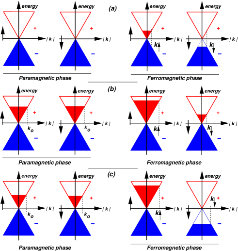
Figure 2: Occupied and empty states in the paramagnetic and ferromagnetic ground states of Dirac fermions (a) half-filling case; (b) finite doping and one type of carrier in the ferromagnetic phase; (c) finite doping and two types of carriers in the ferromagnetic phase.

As function of the Fermi wave vector, $k_{\rm F}$, the kinetic energy of the unpolarized state is:

$$\langle{\cal H}_{\rm kin}\rangle=K=-\frac{A}{3\pi}v_{\rm F}\hbar(k_{c}^{3}-k_{\rm F}^{2})\,,$$ (14)

and the exchange energy, for any doping, as determined from Eq.(LABEL:exchange) can be written as

$$E_{ex}= - \frac{A}{(2\pi)^{2}}\frac{e^{2}}{4\epsilon_{0}}\sum_{\sigma}\sum_{\alpha_{a},\alpha_{b}}\int_{0}^{2\pi}d\theta\int kpdkdp$$ (15)

$$\frac{1+\alpha_{a}\alpha_{b}\cos\theta}{|\bm{k}-\bm{p}|}n_{\rm F}^{\sigma,\alpha_{a}}(\bm{k})n_{\rm F}^{\sigma,\alpha_{b}}(\bm{p})\,,$$

where $n_{\rm F}^{\sigma,\alpha_{a}(\alpha_{b})}(\bm{k})$ is the Fermi occupation function, $a(b)$ is the band indice, and $\alpha_{a},\alpha_{b}=\pm 1$.

In the ferromagnetic state the degeneracy of the spin states is lifted and the Fermi momentum of the up and down spin states becomes $k_{\uparrow}$ and $k_{\downarrow}$, respectively. Depending on the values of $k_{\rm F},k_{\uparrow}$ and $k_{\downarrow}$, we can define the three cases shown in Fig. 2. For a doping, $\delta$ per unit area, the number of electrons per Carbon away from half-filling, $n$, can be written as:

$$n=\delta A_{0}\,.$$ (16)

Because of the different values of $k_{\uparrow}$ and $k_{\downarrow}$ the system acquires a spin magnetization, $\mu=g_{s}\mu_{B}m$, where $g_{s}\approx 2$ is the electron gyromagnetic factor, $\mu_{B}$ is the Bohr magneton, and $m=s\,A_{0}$ with $s=n_{\uparrow}-n_{\downarrow}$, is the spin polarization. Notice that the maximum polarization allowed is $m=2-2n$ since each added (subtracted) electron leads to a doubly (empty) Carbon $\pi$ orbital.

The total exchange energy, eq.(15), can be split into intra- and inter-band contributions. In many band systems where the different bands arise from different atomic orbitals, the overlap integral between Bloch states corresponding to different bands can be neglected, and, consequently, there are no inter-band contributions to the exchange energy. An analogous effect arises when the different bands are localized at different sites of the lattice, as in the gapful case to be considered below. There are also situations where the different bands arise from the same orbitals at the same sites, but their phases in a region much larger than the unit cell are such that the overlap integral vanishes. This is the case for the two different Dirac cones which can be defined in the honeycomb lattice. We do not need to include in eq.(15) terms due to interactions between electrons near different Dirac points of the Brillouin Zone.

The case studied here, where the overlap between Bloch states in different bands cannot be neglected, and a corresponding term in the exchange energy has to the included is generic to narrow gap semiconductors, and this term may be important in lightly doped materials.

It is worth noting that these inter-band exchange effect arise from the non local nature of the exchange interaction. They cannot be studied when the exchange energy is approximated by a local term which only depends on the total charge density.

III.1.2 Undoped case: $n=0$

The Fermi level in the paramagnetic case is at $\epsilon_{\rm F}=0$, and the bands are half-filled. Then, in the paramagnetic state one has $k_{\uparrow}=k_{\downarrow}$. When the system polarizes the magnetization is such that $k_{\uparrow}=\sqrt{2\pi s}$ and the change in energy relative to the paramagnetic state is given by:

$$\Delta E = \Delta K+\Delta E_{\rm ex}=\frac{A_{0}}{3\pi}\hbar v_{\rm F}k_{\uparrow}^{3}$$ (17)

$$- \frac{A_{0}}{(2\pi)^{2}}\frac{e^{2}}{4\epsilon_{0}}\left[2k_{\uparrow}^{3}R_{1}(1)-4k_{c}k_{\uparrow}^{2}R_{0}\left(\frac{k_{\uparrow}}{k_{c}}\right)\right]\,,$$

where the functions $R_{n}(x)$ are defined in the Appendix A. Unfortunately it is not possible to find an analytical expression (using elementary functions) for the energy change as a function of the electron polarization $s=k_{\uparrow}^{2}/(2\pi)$. For $k_{\uparrow}\ll k_{c}$, the leading contribution comes from the expansion of function $R_{0}(x)\approx-x\ln(x)$ for $x\ll 1$ (see Appendix A). Hence, the exchange energy increases as the polarization increases, and a ferromagnetic state with small magnetization is not favored. This effect can be cast as a logarithmic renormalization of the Fermi energy, which reduces the density of states near the Fermi level, and suppresses the tendency toward ferromagnetismGonzález et al. (1999).

At large magnetizations, $k_{c}^{2}/s\sim 1$, the kinetic energy contribution tends to a term proportional to $v_{\rm F}k_{c}^{3}$ and the exchange contribution becomes negative and proportional to $-(e^{2}k_{c}^{3})/\epsilon_{0}$. The exchange term dominates, and the system undergoes a discontinuous transition to a state with polarization of order unity when:

$$g_{c}=\frac{e^{2}}{\hbar v_{\rm F}\epsilon_{0}}\geq\frac{16\pi}{6R_{1}(1)-12R_{0}(1)}\simeq 5.3\,,$$ (18)

which gives the critical coupling $g_{c}(n=0)\approx 5.3$ for the appearance of ferromagnetism in the clean system, as shown in Fig.1.

III.1.3 Doped case, $n\neq 0$, one type of carrier in the ferromagnetic phase

In this case the doping, $\delta$, and magnetization, $s$, are such that $k_{\rm F}=\sqrt{2\pi\delta}$ in the paramagnetic paramagnetic phase, and $k_{\uparrow}=\sqrt{2\pi(s+\delta)}$ and $k_{\downarrow}=\sqrt{2\pi(s-\delta)}$ in the ferromagnetic phase. In this phase there is only one type of carriers, either electrons or holes. The change in energy between the paramagnetic and ferromagnetic phase is:

$$\Delta E = \Delta K+\Delta E_{\rm ex}=\frac{A_{0}}{6\pi}v_{F}\hbar(k_{\uparrow}^{3}+k_{\downarrow}^{3}-2k_{\rm F}^{3})$$ (19)

$$- \frac{A_{0}}{(2\pi)^{2}}\frac{e^{2}}{\epsilon_{0}}\left[k_{\uparrow}^{3}R_{1}(1)+k_{\downarrow}^{3}R_{1}(1)-2k_{\rm F}^{3}R_{1}(1)\right.$$

$$+ 2k_{c}k_{\downarrow}^{2}R_{2}\left(\frac{k_{\downarrow}}{k_{c}}\right)+2k_{c}k_{\uparrow}^{2}R_{2}\left(\frac{k_{\uparrow}}{k_{c}}\right)$$

$$- 4\left.k_{c}k_{\rm F}^{2}R_{2}\left(\frac{k_{\rm F}}{k_{c}}\right)\right]\,.$$

The behavior of the energy change as a function of the spin polarization is shown in left hand pannel in Fig.3 for points $1$ and $2$ of the phase diagram in Fig.1. Notice that the transition between the paramagnetic phase (point $2$) to the ferromagnetic phase (point $1$) is discontinuous with full polarization, $m=2-2n$. In this case analytical expansion when $s\ll\delta$ is now possible. For $k_{\rm F},k_{\uparrow},k_{\downarrow}\ll k_{c}$ the value of the exchange contribution is dominated by the expansion of $R_{2}(x)$ (see Appendix A). The contribution of the exchange interaction to the term proportional $s^{2}$ is positive at low doping, and a continuous ferromagnetic transition is not possible. This contribution becomes negative only for $n=\delta A_{0}\geq 0.059$. As in the previous case, we can also analyze the system energy for large values of the magnetization. We obtain an instability to a ferromagnetic state with full polarization ($m=2-2n$), which for $n\neq 0$ leads to a state with both electron and hole carriers with different Fermi surface areas. The dependence of the coupling constant $g_{c}$ on $n$ is given in Fig.1 by the dashed line. (See more on the conclusions about a speculative scenario for the origin of electrons and hole pockets in graphite.)

III.1.4 Doped case, $n\neq 0$, two types of carriers in the ferromagnetic phase

In this case the calculation is analogous to the previous one. The change in energy in this case is given by:

$$\Delta E = \Delta K+\Delta E_{\rm ex}=\frac{A_{0}}{6\pi}v_{F}\hbar(k_{\uparrow}^{3}-k_{\downarrow}^{3}-2k_{\rm F}^{3})$$ (20)

$$- \frac{A_{0}}{(2\pi)^{2}}\frac{e^{2}}{\epsilon_{0}}\left[k_{\uparrow}^{3}R_{1}(1)+k_{\downarrow}^{3}R_{1}(1)-2k_{\rm F}^{3}R_{1}(1)\right.$$

$$- 2k_{c}k_{\downarrow}^{2}R_{1}\left(\frac{k_{\downarrow}}{k_{c}}\right)+2k_{c}k_{\uparrow}^{2}R_{2}\left(\frac{k_{\uparrow}}{k_{c}}\right)$$

$$- \left.4k_{c}^{2}R_{2}\left(\frac{k_{\rm F}}{k_{c}}\right)\right]\,.$$

As in the two previous cases, the leading term when $k_{\rm F},k_{\uparrow},k_{\downarrow}\ll k_{c}$ is due to the expansion of the function $R_{2}(x)$, which leads to an increase in the exchange energy, which is detrimental for ferromagnetism. The energy change as a function of $m$ is shown in the right hand panel of Fig.3. We show the energy at points $3$ (paramagnetic) and $4$ (ferromagnetic) of Fig. 1. The transition in this case is second order with only partial polarization, $m<n$. As a consequence only one type of carries exist. The dependence of the coupling constant $g_{c}$ on $n$ is given in Fig.1 by the solid line.

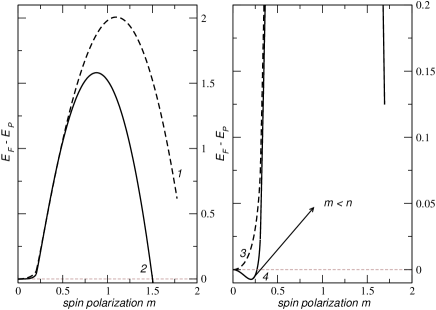
Figure 3: Behavior of the energy curves as function of the magnetization for the points marked in the phase diagram of Fig.1.

III.2 Gapful system

A gap can open in the Dirac spectrum when the two sites in the unit cell of the honeycomb lattice model become inequivalent equivalent. In this case, the kinetic energy Hamiltonian, Eq.(2) changes to:

$${\cal H}_{\rm kin}(\bm{k})\equiv\left(\begin{array}[]{cc}\Delta&v_{\rm F}\hbar(k_{x}+ik_{y})\\ v_{\rm F}\hbar(k_{y}-k_{y})&-\Delta\end{array}\right)\,,$$ (21)

which leads to the modified dispersion relation,

$$\epsilon_{\bm{k}}=\pm\sqrt{\Delta^{2}+(\hbar v_{\rm F}|{\bm{k}}|)^{2}}\,.$$ (22)

For wavevectors such that $\hbar v_{\rm F}|{\bm{k}}|\gg\Delta$ the energies and wavefunctions are essentially the ones found in the absence of the gap, as discussed previously. If the filling is such that the Fermi wavevector satisfies this conditions, but $k_{\rm F}\ll k_{c}$ the analysis presented earlier remains valid. At sufficiently low fillings, $\hbar v_{\rm F}|k_{\rm F}|\ll\Delta$, the dispersion relation, Eq.(21) can be approximated by:

$$\epsilon_{\bm{k}}\approx\pm\Delta\pm\frac{(\hbar v_{\rm F}|\bm{k}|)^{2}}{2\Delta}\,,$$ (23)

and the bands depend quadratically on the wave vector and we can define an effective mass $m^{*}=\Delta/v_{\rm F}^{2}$. Hence, the contribution of the kinetic energy to the polarization energy is formally similar to that obtained for an 2D electron gas with parabolic dispersion discussed extensively in the literature. In this case, the spinor wave function becomes:

$$\Psi_{\bm{k},\sigma}(\bm{r})\simeq\left(\begin{array}[]{c}e^{i\bm{k}\bm{r}}\\ 0\end{array}\right)\chi_{\sigma}\,,$$ (24)

for the upper sub-band, while the weight of the spinor is concentrated on $\psi_{b}$, Eq.(10), for the lower sub-band. This change modifies significantly the spinor overlap factor in the calculation of the exchange integral, Eq.(15). The overlap between Bloch states in different bands for momenta near the Fermi points vanishes (see the discussion at the end of Section III.A.1). These states do not give rise to inter-band contributions. The only inter-band contributions which need to be included are due to interactions between states far from the chemical potential among themselves, and between these states at the bottom of the lower band and those at the Fermi level. These terms are not modified when the system is polarized, and they do not contribute to the exchange instability. The remaining intraband term is equivalent to that derived for the electron gas with parabolic dispersion relation. The change in energy when the polarized state is formed can be written as

$$\Delta E = \Delta K+\Delta E_{\rm ex}=\frac{A_{0}}{8\pi}\frac{v_{\rm F}^{2}}{2\Delta}(k_{\uparrow}^{4}+k_{\downarrow}^{4}-2k_{\rm F}^{4})$$ (25)

$$- \frac{A_{0}}{(2\pi)^{2}}\frac{e^{2}}{\epsilon_{0}}\frac{4}{3}(k_{\uparrow}^{3}+k_{\downarrow}^{3}-2k_{\rm F}^{3})\,,$$

As in the usual case of the 2D electron gas, the system shows an instability toward a ferromagnetic state when $k_{\rm F}\leq(16\Delta e^{2})/(\pi v_{\rm F}^{2}\epsilon_{0})$. In agreement with the previous discussion, this instability vanishes when $\Delta\rightarrow 0$.

III.3 The effect of disorder

We approximate the effects of disorder on the average electronic structure by means of the CPA Soven (1967). This approximation describes the effects of disorder on the electronic structure by means of a local self energy, $\Sigma(\omega)$ which is calculated self consistently. While CPA cannot describe localization effects, it still gives very good results for the physical properties of graphene nun .

The total energy, including the exchange contribution, can be expressed in terms of single particle Green’s functions, which are calculated within the CPA. The main steps of the calculation are sketched in Appendix B. We assume that the disorder is induced by vacancies, as likely to occur in samples treated by proton bombardment. The amount of disorder is parametrized by the concentration o vacancies, $n_{\rm vac}$. The CPA leads to a density of states which is finite at $\omega=0$, and decays for $\omega\gg v_{\rm F}n_{\rm vac}^{1/2}$nun .

Assuming that $\lim_{\omega\rightarrow 0}{\rm Im}\Sigma(\omega)=\Sigma_{0}\sim(\hbar v_{\rm F})/l$, where $l$ is the average distance between vacancies nun the calculations in Appendix B admit some simplifications. If the concentration of vacancies is small, $\Sigma_{0}\ll\hbar v_{\rm F}|k_{c}|$. At large energies the CPA result vanishes quite fast as a function of energy, $\lim_{\omega\rightarrow\pm\hbar v_{\rm F}|k_{c}|}\Sigma(\omega)=0$. Disorder only changes significantly the results obtained for a clean plane if $\epsilon_{\rm F}\ll\Sigma_{0}$. This regime corresponds to electronic densities such that $|n|\ll n_{0}=(\Sigma_{0}/\hbar v_{\rm F})^{2}/2\pi$.

In this limit, we can approximately write

$$n_{\bf\vec{k}}^{\pm}\approx\left\{\begin{array}[]{lr}0&\hbar v_{\rm F}|\bm{k}|\gg\Sigma_{0}\,,\\ 1/2+\frac{\epsilon_{\rm F}}{\pi\Sigma_{0}}&\hbar v_{\rm F}|\bm{k}|\ll\Sigma_{0}\,,\end{array}\right.\,.$$ (26)

where the $\pm$ index refers to the two subbands of the noninteracting system (see Appendix B).

The total density of carriers is obtained by integrating this expression over ${\bf\vec{k}}$ (see Appendix B). Finally, we can also calculate the density of states per unit area and unit energy, which, for $|\omega|\leq\Sigma_{0}$, becomes a constant:

$$D(\omega)=D_{0}\approx\frac{1}{2\pi}\frac{\Sigma_{0}}{v_{\rm F}^{2}}\log\left(\frac{\hbar v_{\rm F}k_{c}}{\Sigma_{0}}\right)\,,\hskip 14.22636pt|\omega|,|\epsilon_{\rm F}|\ll\Sigma_{0}\,,$$ (27)

A constant density of states implies that the total number of carriers scales as $n\approx D_{0}\epsilon_{\rm F}$, instead of the relation $n\propto\epsilon_{\rm F}^{2}$ obtained for the clean system.

From equations (26) and (27) we can infer that both the kinetic energy and the exchange energy depend quadratically on the density of carriers, since $K(n)-K(0)$ and $E_{\rm exch}(n)-E_{\rm exch}(0)$ scale as $\epsilon_{\rm F}^{2}(n)\sim n^{2}$. In addition, we know that for $n\approx n_{0}$ the values of $K(n)$ and $E_{\rm exch}(n)$ should be comparable to those obtained in the absence of disorder. Then, we can write:

$$K(n) \approx c_{\rm kin}\frac{2A_{0}\Sigma_{0}^{3}}{3\pi\hbar^{2}v_{\rm F}^{2}}\left(\frac{n}{n_{0}}\right)^{2},$$

$$E_{\rm exch}(n) \approx -c_{\rm exch}\frac{A_{0}e^{2}\Sigma_{0}^{3}}{3\pi^{2}\epsilon_{0}\hbar^{3}v_{\rm F}^{3}}\left(\frac{n}{n_{0}}\right)^{2},$$ (28)

where $c_{\rm kin}$ and $c_{\rm exch}$ are numerical constants of order unity. In a spin polarized system, we have:

$$E_{\rm tot}(n,m)=\frac{1}{2}\left[K(n+m)+K(n-m)+E_{\rm exch}(n+m)+E_{\rm exch}(n-m)\right],$$ (29)

so that:

$$\Delta E=\Delta K+\Delta E_{\rm exch}=c_{\rm kin}\frac{2A_{0}\Sigma_{0}^{3}}{3\pi\hbar^{2}v_{\rm F}^{2}}\left(\frac{m}{n_{0}}\right)^{2}-c_{\rm exch}\frac{A_{0}e^{2}\Sigma_{0}^{3}}{3\pi^{2}\epsilon_{0}\hbar^{3}v_{\rm F}^{3}}\left(\frac{m}{n_{0}}\right)^{2}\,.$$ (30)

The ferromagnetic phase is stable provided that:

$$g_{c,{\rm disorder}}=\frac{e^{2}}{\epsilon_{0}\hbar v_{\rm F}}>\frac{2\pi c_{\rm kin}}{c_{\rm exch}},$$ (31)

This result implies that, if $n\ll n_{0}$ the critical coupling is independent of the amount of disorder.

We have estimated the ratio $c_{\rm exch}/c_{\rm kin}$ performing numerically the calculation described in Appendix B for suficiently low carrier concentration and density of vacancies. We find:

$$g_{c,{\rm disorder}}=\frac{e^{2}}{\epsilon_{0}\hbar v_{\rm F}}\simeq 3.8\,,$$ (32)

indicating that in the case of disorder ferromagnetism is stabilized at a smaller value of the Coulomb interaction. Thus, we can conclude that, at least in CPA, ferromagnetism will be enhanced when disorder is present, in agreement with the experimental data Esquinazi et al. (2003); dis .

The enhancement of the tendency towards ferromagnetism in the presence of disorder is due to the increase in the density of states at low energies. The existence of these states implies that a finite polarization can be achieved with a smaller cost in kinetic energy, in a qualitatively similar way to the Stoner criterium which explains itinerant ferromagnetism in the presence of short range interactions.

IV Discussion and Conclusions

We have analyzed the ferromagnetic instabilities induced by the exchange interaction in a system where the electronic structure can be approximated by the 2D Dirac equation, as it is the case for isolated graphene planes.

In pure graphene we have found that, as a function of doping, a ferromagnetic transition is possible when the coupling constant is sufficiently large. Our findings are summarized in the zero temperature phase diagram presented in Fig. 1. In this figure we represent the critical coupling $g_{c}$ as function of the doping $n$. There are two different regions in the phase diagram. For small doping, $n<0.2$ the transition is first order, leading to a ferromagnetic phase with spin polarization $m=2-2n$ and two types of carriers (electrons and holes). For doping larger than $n>0.2$ the transition becomes of second order with a magnetization smaller than the doping $n$ and one type of carrier (electrons or holes). The connection between the magnetization and the carrier type is unique to the Dirac fermion problem. We should emphasize that our calculation for the Dirac fermion problem is at the same level of the one performed by Bloch, and therefore it is to be expected that an exact solution of this problem will modify quantitatively the phase diagram analyzed here. It is also worth remarking that the electronic structure shown in panel of (c) Fig. 2 shows that, in the ferromagnetic phase, a nominally half filled system has electron and hole pockets. The existence of these pockets does not depend on the presence of intarlayer coherence, however

We have also analyzed the effect of the exchange interaction in disordered systems using the CPA. A continuous transition into a ferromagnetic phase is possible, and the coupling required for its existence is reduced with respect to the clean case. This tendency can be qualitatively explained by noting that the disorder leads to an increase of the density of states at low energies, making the system more polarizable. This explanation is rather general, and it should not depend on the way the effects of disorder are approximated.

Finally, one would ask how our results can be translated for the experiments in disordered graphite Esquinazi et al. (2003); dis . If we naively think of graphite as a stacking of isolated graphene planes we can estimate the value of the coupling constant for graphite to be $g\sim 2.8$ (for $\epsilon_{0}\approx 1$) Brandt et al. (1988), and therefore far away from the ferromagnetic region (corresponding to the dotted line in Fig.1). The presence of disorder will definitely bring the value of the critical coupling to lower values and according to our calculations $g_{c,{\rm disorder}}\approx 3.8$ would put dirty graphite at the borderline of a ferromagnetic instability.

Nevertheless, the picture of graphene as a non-interacting stacking of graphene planes is certainly incorrect. Because of the absence of screening, long-range forces will play a major role, and the graphene planes will interact via van der Waals interactions. The problem of ferromagnetism in graphite still depends on the better understanding of the coupling between graphene planes. More work has to be developed in order to understand the problem of ferromagnetism in graphite. In any case, our results here are valid for single graphene planes and it would be very interesting to investigate whether graphitic devices Novoselov et al. (2004); Zhang et al. (2004, 2005); Berger et al. (2004) studied recently can sustain any form of ferromagnetism.

V Acknowledgments

N.M.R.P and F. G. are thankful to the Quantum Condensed Matter Visitor’s Program at Boston University. A.H.C.N. was partially supported through NSF grant DMR-0343790. N. M. R. Peres would like to thank Fundação para a Ciência e Tecnologia for a sabbatical grant partially supporting his sabbatical leave.

Appendix A Calculation of the exchange integral

The three dimensional integral in Eq.(15) can be written as a combination of integrals of the form:

$$R_{n}(a)=\int_{0}^{2\pi}d\alpha\int_{0}^{1}xdx\int_{0}^{1}ydy\frac{{\rm sign}(n)-(-1)^{n}\cos\alpha}{\sqrt{x^{2}+y^{2}a^{2}-2xya\cos\alpha}}\,,$$ (33)

where: $n=0,1,2$, ${\rm sign}(n)$ gives the sign of $n$ and ${\rm sign}(0)=0$. The values of the functions $R_{n}(a)$, for $a=0$, are $R_{0}(0)=0$ and $R_{1}(0)=R_{2}(0)=\pi$. We also have:

$$R_{0}(1) = \frac{2}{3}\left(-2+\pi(\ln 2+1/2)+4{\cal C}-\pi(1+\ln 4)/2\right)$$

$$\simeq 1.109\,,$$

$$R_{1}(1) = 8/3+R_{0}(1)\simeq 3.776\,,$$ (34)

where ${\cal C}\simeq 0.915966$ is the Catalan constant.

Assuming that $0\leq a\leq 1$ we define:

$$R_{n}(a)=\int_{0}^{2\pi}d\alpha[{\rm sign}(n)1-(-1)^{n}\cos\alpha]K(\alpha,a)\,,$$ (35)

where $K(\alpha,a)$ is given by:

$$K(\alpha,a) = \frac{1}{3a^{2}}\left[-(1+a^{3})+(1+a^{2})\sqrt{1+a^{2}-2a\cos\alpha}-(1+a^{3})\cos\alpha\ln(1-\cos\alpha)-a^{3}\cos\alpha\ln a\right.$$ (36)

$$+ \left.\cos\alpha\ln(a-\cos\alpha+\sqrt{1+a^{2}-2a\cos\alpha})-a^{3}\cos\alpha\ln(1-a\cos\alpha+\sqrt{1+a^{2}-2a\cos\alpha})\right]\,$$

This expression allows us to obtain the expansions:

$$R_{0}(a) \simeq \frac{\pi}{3}[-a\ln a+S_{0}(a)]\,,$$ (37)

$$R_{n}(a) \simeq \frac{\pi}{3}[3+(-1)^{n}a\ln a+S_{n}(a)]\,,$$ (38)

for $n=1,2$ and

$$S_{0}(a) = \left(2\ln 2-\frac{1}{6}\right)a-\frac{9}{80}a^{3}-\frac{45}{1792}a^{5}$$ (39)

$$- \frac{175}{18432}a^{7}\,,$$

$$S_{n}(a) = -(-1)^{n}\left(2\ln 2-\frac{1}{6}\right)a-\frac{3}{8}a^{2}+(-1)^{n}\frac{9}{80}a^{3}$$ (40)

$$- \frac{3}{64}a^{4}+(-1)^{n}\frac{45}{1792}a^{5}-\frac{15}{1024}a^{6}$$

$$+ (-1)^{n}\frac{175}{18432}a^{7}\,.$$

Note that $R_{1}(a)-R_{2}(a)=2R_{0}(a)$ is always satisfied.

Appendix B Calculation of the exchange energy in the presence of disorder.

We write the one-electron energies in the absence of interactions and disorder as:

$$\epsilon_{\bm{k}}^{\pm}=\pm v_{\rm F}({\bm{k}})\,,$$ (41)

up to some cutoff $k_{c}$, where the two signs correspond to the two bands in the electronic spectrum. Using the CPA, the one electron Green’s function can be written as:

$$G^{\pm}({\bm{k}},\omega)=\frac{1}{\omega-\Sigma(\omega)-\epsilon_{\bm{k}}^{\pm}}\,.$$ (42)

The occupancy of a given state at fixed chemical potential, $\epsilon_{\rm F}$, is:

$$n_{\bm{k}}^{\pm}=\int_{-\omega_{c}}^{\epsilon_{\rm F}}\frac{1}{\pi}{\rm Im}G^{\pm}({\bm{k}},\omega)d\omega\,,$$ (43)

where a frequency cutoff, $\omega_{c}$ is also defined.

The total number o electrons, $n$, and the kinetic energy can be written as:

$$n = \sum_{\alpha=\pm}\frac{2}{\pi}\int_{0}^{k_{c}}n_{|{\bm{k}}|}^{\alpha}kdk\,,$$

$$K = \sum_{\alpha=\pm}\frac{2}{\pi}\int_{0}^{k_{c}}\alpha\epsilon_{|{\bm{k}}|}n_{|{\bm{k}}|}^{\alpha}kdk\,.$$ (44)

These one-dimensional integrals are calculated numerically. Finally, the exchange energy is:

$$E_{\rm exch}=-\frac{e^{2}}{4\pi^{4}}\int d^{2}{\bm{k}}_{1}\int d^{2}{\bm{k}}_{2}\frac{[n^{+}({\bm{k}}_{1})+n^{-}({\bm{k}}_{2})]^{2}+[n^{+}({\bm{k}}_{1})-n^{-}({\bm{k}}_{2})]^{2}\cos[\phi({\bm{k}}_{1})-\phi({\bm{k}}_{2})]}{|{\bm{k}}_{1}-{\bm{k}}_{2}|}\,,$$ (45)

and:

$$\phi({\bm{k}})=\arctan\left(\frac{k_{y}}{k_{x}}\right)\,.$$ (46)

This expression can be reduced to a three-dimensional integral, which is calculated numerically.

The total energy, $E_{\rm tot}(n)=K(n)+E_{exch}(n)$, can be written as:

$$E_{\rm tot}(n)=E_{\rm tot}(n_{\uparrow})+E_{\rm tot}(n_{\downarrow})\,.$$ (47)

The exchange instability towards ferromagnetism implies that:

$$E_{\rm tot}(n/2-\delta n)+E_{\rm tot}(n/2+\delta n)<2E_{\rm tot}(n/2)\,,$$ (48)

so that:

$$\left.\frac{\partial^{2}E_{\rm tot}}{\partial n^{2}}\right|_{n/2}<0\,.$$ (49)

References

- Bloch (1929) F. Bloch, Z. Physik 57, 549 (1929).
- Iwamoto and Sawada (1962) F. Iwamoto and K. Sawada, Phys. Rev. 126, 887 (1962).
- Misawa (1965) S. Misawa, Phys. Rev. 140, A1645 (1965).
- Ceperley (1978) D. Ceperley, Phys. Rev. B 18, 3126 (1978).
- Ceperley and Alder (1980) D. M. Ceperley and B. J. Alder, Phys. Rev. Lett. 45, 566 (1980).
- Attaccalite et al. (2002) C. Attaccalite, S. Moroni, P. Gori-Giorgi, and G. B. Bachelet, Phys. Rev. Lett. 88, 256601 (2002).
- Ceperley (1999) D. Ceperley, Nature 397, 386 (1999).
- Fisk et al. (2002) D. P. Y. Z. Fisk, J. D. Thompson, H.-R. Ott, S. B. Oseroff, and R. G. Goodrich, Nature 420, 144 (2002).
- Young et al. (1999) D. P. Young, D. Hall, M. E. Torelli, Z. Fisk, J. L. Sarrao, J. D. Thompson, H.-R. Ott, S. B. Oseroff, R. G. Goodrich, and R. Zysler, Nature 397, 412 (1999).
- Esquinazi et al. (2003) P. Esquinazi, D. Spemann, R. Höhne, A. Setzer, K.-H. Han, and T. Butz, Phys. Rev. Lett. 91, 227201 (2003).
- (11) See papers in Carbon-Based Magnetism: an overview of metal free carbon-based compounds and materials, T. Makarova and F. Palacio, eds. (Elsevier, Amsterdam, 2005).
- Ovchinnikov and Shamovsky (1991) A. A. Ovchinnikov and I. L. Shamovsky, Journ. of. Mol. Struc. (Theochem) 251, 133 (1991).
- Harigaya (2001) K. Harigaya, Journ. of Phys. C; Condens. Matt. 13, 1295 (2001).
- Lehtinen et al. (2004) P. O. Lehtinen, A. S. Foster, Y. Ma, A. V. Krasheninnikov, and R. M. Nieminen, Phys. Rev. Lett. 93, 187202 (2004).
- Vozmediano et al. (2005) M. A. H. Vozmediano, M. P. López-Sancho, T. Stauber, and F. Guinea (2005), eprint cond-mat/0505557.
- Brandt et al. (1988) N. B. Brandt, S. M. Chudinov, and Y. G. Ponomarev, in Modern Problems in Condensed Matter Sciences, edited by V. M. Agranovich and A. A. Maradudin (North Holland (Amsterdam), 1988), vol. 20.1.
- Novoselov et al. (2004) K. S. Novoselov, A. K. Geim, S. V. Morozov, D. Jiang, Y. Zhang, S. V. Dubonos, I. V. Gregorieva, and A. A. Firsov, Science 306, 666 (2004).
- Zhang et al. (2004) Y. Zhang, J. P. Small, W. V. Pontius, and P. Kim (2004), eprint cond-mat/0410314.
- Zhang et al. (2005) Y. Zhang, J. P. Small, M. E. S. Amori, and P. Kim, Phys. Rev. Lett. 94, 176803 (2005).
- Berger et al. (2004) C. Berger, Z. M. Song, T. B. Li, X. B. Li, A. Y. Ogbazghi, R. Feng, Z. T. Dai, A. N. Marchenkov, E. H. Conrad, P. N. First, et al., J. Phys. Chem. B 108, 19912 (2004).
- (21) N.M.R. Peres and F. Guinea and A. H. Castro Neto, cond-mat/0506709.
- González et al. (1996) J. González, F. Guinea, and M. A. H. Vozmediano, Phys.Rev.Lett. 77, 3589 (1996).
- Stoner (1947) E. C. Stoner, Rep. Prog. Phys. 11, 43 (1947).
- Khveshchenko (2001) D. V. Khveshchenko, Phys. Rev. Lett. 87, 246802 (2001).
- Gorbar et al. (2002) E. V. Gorbar, V. P. Gusynin, V. A. Miransky, and I. A. Shovkovy, Phys. Rev. B 66, 045108 (2002).
- Goñi et al. (2002) A. R. Goñi, U. Haboeck, C. Thomsen, K. Eberl, F. A. Reboredo, C. R. Proetto, and F. Guinea, Phys. Rev. B 65, 121313 (2002).
- Peres et al. (2004) N. M. R. Peres, M. A. N. Araújo, and D. Bozi, Phys. Rev. B 70, 195122 (2004).
- Sorella and Tossatti (1992) S. Sorella and E. Tossatti, Europhys. Lett. 19, 699 (1992).
- DiVincenzo and Mele (1984) D. P. DiVincenzo and E. J. Mele, Phys.Rev.B 29, 1685 (1984).
- González et al. (1999) J. González, F. Guinea, and M. A. H. Vozmediano, Phys. Rev. B 59, R2474 (1999).
- Soven (1967) P. Soven, Physical Review 156, 809 (1967).