Solitonic Excitations in Linearly Coherent Channels of Bilayer Quantum Hall Stripes

Abstract

In some range of interlayer distances, the ground state of the two-dimensional electron gas at filling factor $\nu=4N+1$ with $N=0,1,2,...$ is a coherent stripe phase in the Hartree-Fock approximation. This phase has one-dimensional coherent channels that support charged excitations in the form of pseudospin solitons. In this work, we compute the transport gap of the coherent striped phase due to the creation of soliton-antisoliton pairs using a supercell microscopic unrestricted Hartree-Fock approach. We study this gap as a function of interlayer distance and tunneling amplitude. Our calculations confirm that the soliton-antisoliton excitation energy is lower than the corresponding Hartree-Fock electron-hole pair energy. We compare our results with estimates of the transport gap obtained from a field-theoretic model valid in the limit of slowly varying pseudospin textures.

I Introduction

It is well known that the ground state of the two-dimensional electron gas (2DEG) in single layer quantum Hall systems near half-odd integer filling factors in Landau levels $N\geq 2$ i.e. for $\nu=9/2,11/2,\ldots$ is a striped state responsible for a strong anisotropy in the conductivity tensor of the 2DEG. This state was predicted on the basis of Hartree-Fock calculationsstripetheory and has been extensively studied experimentally.stripeexperimental

When the interlayer distance, $d$, in a bilayer quantum Hall system at filling factor $\nu$ is large, one expects the system to behave as two isolated two-dimensional electron gases (2DEG) with filling factor $\nu/2$. It is then natural to infer that the ground state of the 2DEG in a bilayer should be a striped state at $\nu=4N+1$ at sufficiently large interlayer distances. On the other hand, it is known that, at $\nu=4N+1$ interlayer interactions can lead to a homogeneous ground state with spontaneous phase coherence between the layers when the interlayer distance is comparable with the separation between electrons in a single layer. One might then conjecture that, as the interlayer separation is decreased, the striped state acquires a certain degree of coherence due to the interlayer interaction. This conjecture was first studied by Brey and Fertigbreystripes who showed that, as $d$ is increased from zero the bilayer ground state goes from a uniform coherent state (UCS) at small interlayer separations to a coherent striped phase (CSP) at $d\geq d_{1}$ and then into a modulated striped state (or anisotropic Wigner crystal) at $d\geq d_{2}$. The interlayer coherence is lost in the modulated stripe state. The range $\left[d_{1},d_{2}\right]$ increases with $N$.Dorra

The coherent striped phase shown in Fig. 1 is a state where charge density waves in the two layers are shifted by $\xi/2$ where $\xi$ is the period of the stripes in one layer. The most interesting aspect of the CSP is that in the regions where the charge densities in both layers “overlap” (in the plane of the two-dimensional electron gas (2DEG)), the electrons are effectively in a linear superposition of states of the form $\left|\psi\right\rangle=\left(\left|R\right\rangle+\left|L\right\rangle\right)/\sqrt{2}$ where $R,L$ indicates the right and left wells. The interlayer coherence is then maintained but only along linearly coherent regions (LCR’s) whose width decreases as $d$ increases. The CSP is most easily represented in the pseudospin language where an up (down) pseudospin is associated with the right (left) well. The CSP is a pseudospin density wave where the pseudospins oscillates in the $xz$ plane and the LCR’s are the one-dimensional regions where the pseudospins lie along the $x$ direction in the $xy$ plane.

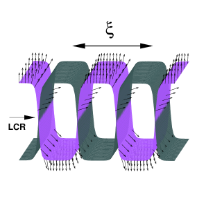
Figure 1: Guiding center density in the right (dark surface) and left (light surface) wells and pseudospin pattern in the coherent stripe phase. The arrow indicates one linearly coherent channel (LCR).

In a previous workcotecspmodes , we have computed the collective excitations of the CSP and showed that the low-energy modes of this phase could be described by an effective pseudospin wave hamiltonian. We have also showncoteparallel that the application of a parallel magnetic field gives rise to a very rich phase diagram for the 2DEG involving commensurate-incommensurate transitions with distinctive signatures in the collective excitations and tunneling $I-V$. A very exhaustive study of the phase diagram of the 2DEG in the presence of a parallel magnetic field, in higher Landau levels, has also been published by Daw-Wei Wang et al.demlerlongarticle ; demlerarticlecourt .

The band structure of the CSP is shown in Fig. 2. In the Hartree-Fock approximation, the energy gap of this system corresponds to the excitation of an electron-hole pair in a coherent channel (a pseudospin flip in the $xy$ plane) and is finite if the tunneling parameter $t\neq 0.$ An estimate of this gap, taking into account some quantum fluctuations, has been done by E. Papa et al.Papamacdo . However, Brey and Fertigbreystripes pointed out that, in analogy with spin (pseudospin) skyrmion excitation in single (double) layer quantum Hall systems at $\nu=1$, the lowest-energy charged excitation should be a pseudospin soliton (or antisoliton) in a coherent channel and the gap should be given by the energy required to create a soliton-antisoliton pair. A pseudospin soliton of charge $q=e$ corresponds to a $2\pi$ rotation of the pseudospin in the $xy$ plane. As for skyrmions or bimerons, the size of these solitons is determined by a competition between tunneling energy (which favors small solitons) and interwell exchange energy and Coulomb interaction which favors slowly varying pseudospin textures (large solitons).

In this work, we compute the energy gap of the CSP due to the excitation of a soliton-antisoliton pair as a function of tunneling and interlayer distance. We use a supercell microscopic unrestricted Hartree-Fock approach to extract the energy of a single soliton from that of a crystal of solitons localized in the LCR’s at filling factor $\nu=4N+1+\Delta\nu$. Our calculation shows that a soliton-antisoliton pair has a lower energy than the electron-hole pair so that these topological excitations will be important in determining the transport properties of the CSP. For completeness, we also compute the energy gap of the CSP using a simple field-theoretic model based on the sine-Gordon Hamiltonian where an exact solution for the pseudospin soliton can be obtained. This model does not contain all the terms included in the microscopic approach, but, for slowly varying pseudospin textures, it should give a fair estimate of the energy gap. We actually improve on this model by taking into account that the channels have a width that depends on the interlayer distance $d$ and also by taking into account the interaction of the pseudospins in different channels and the Coulomb interaction between different portions of the topological charge densities.

The paper is organized as follows. In Sec. II, we describe the phase diagram of the 2DEG in the bilayer system at filling factors $\nu=4N+1$ and $\nu=4N+1+\Delta\nu$ and define the domain of existence of the soliton crystal from which we want to compute the soliton energy. In Sec. III, we introduce the simple field-theoretic model and the exact solution for the pseudospin sine-Gordon solution. Section IV discusses the supercell method that we use to extract the energy of a single soliton from that of a crystal of solitons. The removal of the soliton-soliton energy is discussed in Sec. V. Section VI discusses our numerical results. We conclude in Sec. VII. Details of the derivation of the microscopic expression for the parameters of the field-theoretic model are given in the appendix.

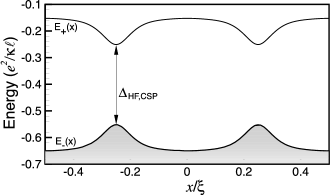
Figure 2: Band structure of the coherent stripe phase. The greyed states represent filled states at $\nu=4N+1$. The Hartree-Fock gap is also indicated. It corresponds to the excitation of an electron-hole pair in one of the linearly coherent channels.

II Phase diagram of the 2DEG around $\nu=4N+1$

In this section, we review the phase diagram of the 2DEG at filling factor $\nu=4N+1$ where the coherent striped state is found and at filling factors slightly above $\nu=4N+1$ in order to find the range of interlayer distances where a crystal of solitons localized in the LCR’s is stable. We need the energy of this soliton lattice in order to compute the gap energy as we explained in the introduction. To establish the phase diagram, we compute the energy of different electronic phases in the Hartree-Fock approximation in order to find the one that minimizes the total energy at a given value of $\nu,d,$ and $t$. The order parameters for the different phases are the expectation values of the density operator projected onto the Landau level $N$ of the partially filled Landau level (the guiding center density), i.e.,

$$\left\langle\rho_{N}^{i,j}(\mathbf{q})\right\rangle = \frac{1}{N_{\phi}}\sum_{X,X^{\prime}}e^{-iq_{x}(X+X^{\prime})/2}\delta_{X,X^{\prime}-q_{y}\ell^{2}}$$

$$\times\left\langle c_{X,i,N}^{\dagger}c_{X^{\prime},j,N}\right\rangle,$$

where $i,j$ are layer indices and $X,~{}X^{\prime}$ are guiding center coordinatescotemethodewc . We make the usual approximation of assuming that the filled levels are inert. We also neglect Landau level mixing and assume that the electron gas in the partially filled level is fully spin polarized. In a crystal phase, $\left\langle\rho_{N}^{i,j}(\mathbf{q})\right\rangle$ is non zero only for $\mathbf{q=G}$ where $\mathbf{G}$ is a reciprocal lattice vector of the crystal. Defining the Hartree and Fock interactions

$$H_{i,j}(N,M;\mathbf{q})=\frac{1}{q\ell}\Lambda_{i,j}(\mathbf{q})e^{-q^{2}\ell^{2}/2}L_{N}^{0}\left(\frac{q^{2}\ell^{2}}{2}\right)L_{M}^{0}\left(\frac{q^{2}\ell^{2}}{2}\right),$$ (2)

and

$$X_{i,j}(N,M;\mathbf{q})=\frac{\left[\min\left(M,N\right)\right]!}{\left[\max\left(M,N\right)\right]!}\int_{0}^{\infty}dy\left(\frac{y^{2}}{2}\right)^{\left|N-M\right|}e^{-y^{2}/2}\left[L_{\min\left(N,M\right)}^{\left|N-M\right|}\left(\frac{y^{2}}{2}\right)\right]^{2}\Lambda_{i,j}\left(\frac{y}{\ell}\right)J_{0}\left(q\ell y\right),$$ (3)

where $L_{N}^{M}\left(x\right)$ is a generalized Laguerre polynomial, $J_{0}\left(x\right)$ is the zeroth-order Bessel function of the first kind and the form factor

$$\Lambda_{i,j}=\begin{cases}1,&\text{if $i=j$},\\ e^{-qd},&\text{if $i\neq j$},\end{cases}$$ (4)

the Hartree-Fock energy per electron at total filling factor $\nu=4N+\widetilde{\nu}$ can be written as

$$\frac{E}{N_{e}}=\varepsilon\left(\frac{e^{2}}{\kappa\ell}\right),$$ (5)

with

$$\varepsilon = -\frac{2\widetilde{t}}{\nu}\mathrm{Re}\left[\langle\rho_{N}^{R,L}(0)\rangle\right]$$

$$+\frac{1}{2\nu}\sum_{i,j}\sum_{\mathbf{G}\neq 0}H_{i,j}\left(N,N,\mathbf{G}\right)\left\langle\rho_{N}^{i,i}\left(-\mathbf{G}\right)\right\rangle\left\langle\rho_{N}^{j,j}\left(\mathbf{G}\right)\right\rangle$$

$$-\frac{1}{2\nu}\sum_{i,j}\sum_{\mathbf{G}}X_{i,j}\left(N,N,\mathbf{G}\right)\left\langle\rho_{N}^{i,j}\left(-\mathbf{G}\right)\right\rangle\left\langle\rho_{N}^{j,i}\left(\mathbf{G}\right)\right\rangle$$

$$-\frac{2}{\nu}\sum_{n<N}\sum_{n^{\prime}<N}X_{R,R}\left(n,n^{\prime},0\right)$$

$$-\frac{1}{\nu}\sum_{n<N}X_{i,i}\left(n,N,0\right)\widetilde{\nu}.$$

In this last equation, $N_{e}$ is the total number of electrons in the 2DEG, $\widetilde{t}$ is the tunneling strength (in units of $\left(e^{2}/\kappa\ell\right)$, with $\kappa$ the dielectric constant of the host material and $\ell=\sqrt{\hbar c/eB}$ the magnetic length).

The last two terms in Eq. (II) give the interaction between electrons in the filled levels and between electrons in the filled levels and electrons in the partially filled level $N$. As we will show later, the filled levels contribute to the quasiparticle energies, but not to the charge gap.

The set of $\langle\rho_{N}^{i,j}(\mathbf{G})\rangle$’s corresponding to one particular electronic phase is found by solving the equation of motion for the one-particle Green’s function in the Hartree-Fock approximation. The method is described in detail in Ref. cotemethodewc, .

The band structure of the CSP contains two bands $E_{\pm}\left(X\right)$, as shown in Fig. 2. At exactly $\nu=4N+1$, the lowest-energy band is completely filled and the system is gapped even in the absence of tunneling. In fact, in the uniform coherent state that occurs for values of $d$ for which stripe ordering had not set in, the band structure consists of two straight lines separated by a gap $\Delta_{UCS}=\left(2\widetilde{t}+2X_{R,L}(N,N;0)\right)\left(e^{2}/\kappa\ell\right)$ with $\Delta_{UCS}\rightarrow 2\widetilde{t}$ as $d\rightarrow\infty.$ In the CSP, the energy bands are periodically modulated in space with the maxima (minima) of the valence (conduction) band at the locations of the LCR’s. At the Hartree-Fock level, the energy gap is the energy needed to excite an electron from a maximum of the valence band to a minimum of the conduction band. This excitation corresponds to a single spin flip localized in one LCR. The decrease in the HF gap in the CSP is due not so much to the reduction of $X_{R,L}(N,N;0)$ with $d$ as to the increase in intralayer correlations that increases the with of the modulations in $E_{\pm}\left(X\right)$. As $d$ increases, the charge modulations get sharper up to the point where the stripes become square waves at very large $d$. Correspondingly, the width of the LCR’s decreases with $d$ since interwell coherence and charge modulation compete with each other.

In analogy with the excitations of skyrmions in single quantum well and bimerons in bilayer systems at $\nu=1$, Brey and Fertigbreystripes noted that a lower-energy excitation could be achieved by exciting a pseudospin soliton in the LCR instead of a simple electron-hole pair. The pseudospin soliton corresponds to a $2\pi$ rotation of the pseudospin in one LCR. A slowly varying pseudospin configuration like that in a soliton has lower exchange energy than a single pseudospin flip but the cost in tunneling energy is increased. As for skyrmions or bimerons, an optimal size for the soliton is obtained at given values of $\nu,d$ and $t$. The energy cost for this optimal soliton should be compared with the Hartree-Fock electron-hole pair excitation to determine whether or not these topological excitations are energetically favorable.

In a quantum Hall system, the relation between the charge density of the solitons and their pseudospin texture (at $\widetilde{\nu}=1$) is given by the Pontryagian densitymacdobible

$$\delta\left\langle\rho\left(\mathbf{r}\right)\right\rangle=\frac{1}{8\pi N_{\phi}}\varepsilon_{abc}S_{a}\left(\mathbf{r}\right)\varepsilon_{ij}\partial_{i}S_{b}\left(\mathbf{r}\right)\partial_{j}S_{c}\left(\mathbf{r}\right),$$ (7)

where $\varepsilon_{ij}$ and $\varepsilon_{abc}$ are antisymmetric tensors and $\mathbf{S}\left(\mathbf{r}\right)$ is a classical field with unit modulus representing the pseudospins and $\delta\left\langle\rho\left(\mathbf{r}\right)\right\rangle$ is the guiding-center density. If we write a general solution as

$$S_{x}\left(\mathbf{r}\right) = \sin\theta\left(\mathbf{r}\right)\cos\varphi\left(\mathbf{r}\right),$$ (8)

$$S_{y}\left(\mathbf{r}\right) = \sin\theta\left(\mathbf{r}\right)\sin\varphi\left(\mathbf{r}\right),$$ (9)

$$S_{z}\left(\mathbf{r}\right) = \cos\theta\left(\mathbf{r}\right),$$ (10)

then the induced density takes the simple form

$$\delta\rho\left(\mathbf{r}\right)=\frac{1}{4\pi N_{\phi}}\sin\theta\left(\mathbf{r}\right)\left[\nabla\varphi\left(\mathbf{r}\right)\times\nabla\theta\left(\mathbf{r}\right)\right]\cdot\widehat{\mathbf{z}}.$$ (11)

In a LCR, the polar angle of the pseudospins $\theta=\pi/2$. If a soliton is present in this LCR, then $\varphi\left(\mathbf{r}\right)$ rotates by $\pm 2\pi$ along the channel (oriented in the $y$ direction). As discussed below, this is a generalization of a soliton in the sine-Gordon modelrajaraman . We also have that, in the CSP, $\nabla\theta\left(\mathbf{r}\right)\neq 0$ in the LCR’s and so the solitons carry a charge by virtue of Eq. (11).

In the case where pseudospin solitons are the lowest-energy excitations of the CSP, we expect that the ground state at $\nu=4N+\widetilde{\nu}$ will be a crystal of solitons localized in the LCR’s. Table I shows that the range of interlayer distances where the CSP is the system’s ground state at $\nu=4N+1$ increases with the Landau level index. In this work, we choose to study the phase diagram in Landau level $N=2$. We show in Fig. 3 the energy per electron for different electronic phases in $N=2$ as a function of interlayer distances and for three values of the tunneling parameter $\widetilde{t}=0,0.01$ and $0.06.$ The filling factor is $\nu=9.2$. The contribution from the filled levels is not included in this calculation since it depends only on $\nu$ and is thus the same for all phases. At small interlayer distances, where the ground state at $\nu=9$ is a UCS, the ground state at $\nu=9.2$ is a one-component hexagonal Wigner crystal (HWC). In this phase, a crystal of electrons of pseudospin $S_{x}=-1/2$ and filling $\widetilde{\nu}=0.2$ sits on top of a liquid of pseudospins $S_{x}=+1/2$ and filling $9.0$. There is no pseudospin texture in that state and, in particular, no bimerons in contrast with the situation in the lowest Landau levelbreybimeron where the ground state is a crystal of bimerons. In fact, we find that bimeron excitations are not relevant in $N=2$ even in the limit of vanishing $\widetilde{t}$.

Landau level	$d_{1}/\ell$	$d_{2}/\ell$	$D/\ell$
0	1.2	1.65	0.45
1	0.8	1.45	0.65
2	0.6	1.6	1.00

Table 1: Critical interlayer distances $d_{1}/\ell$ and $d_{2}/\ell$ at $\widetilde{t}=0$ for the transition UCS-CSP and CSP-modulated striped state. The last column gives the range of interlayer distances $D/\ell=d_{2}/\ell-d_{1}/\ell$ for which the CSP is the ground state in Landau level $N.$

For interlayer distances where the CSP is found at $\nu=9$, the ground state of the 2DEG at $\nu=9.2$ is a centered crystal of pseudospin solitons localized in the LCR’s. We note that there are many possible choices for the lattice structure of this crystal, since solitons may or may not be present in every LCR, depending on the commensuration of the lattice of solitons and the underlying stripe state, and it is likely that there are phase transitions among these different states as the filling factor is varied. For the choice of parameters in this study, the lowest energy state has solitons in every channel. We found however that a similar state with solitons in every second channel but with the same filling factor has very nearly the same energy.

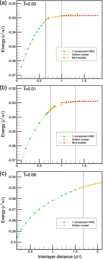
Figure 3: Hartree-Fock ground state energy per electron as a function of interlayer distances at filling factor $\nu=9.2$ and for (a) $\widetilde{t}=0$; (b) $\widetilde{t}=0.01$; (c) $\widetilde{t}=0.06$. The vertical lines indicate the position of the phase transitions.

Figure 4 shows an example of the charge distribution as well as the pseudospin texture associated with a centered rectangular soliton crystal. Since the focus of this study is on the energetics of single solitons, we will use only the structure illustrated in Fig. 4 for our quantitative analysis below.

At large interlayer distances, we find that the ground state of the 2DEG at $\nu=9.2$ is a superposition of two shifted triangular bubble crystalsstripetheory with partial filling $\widetilde{\nu}=0.6$ in each well. Because $\widetilde{\nu}>0.5$ the bubbles are clusters of holes and not electrons. We find that the number of holes per bubble is $M=3$ in agreement with previous Hartree-Fock calculation in single quantum well systemscotebubble .

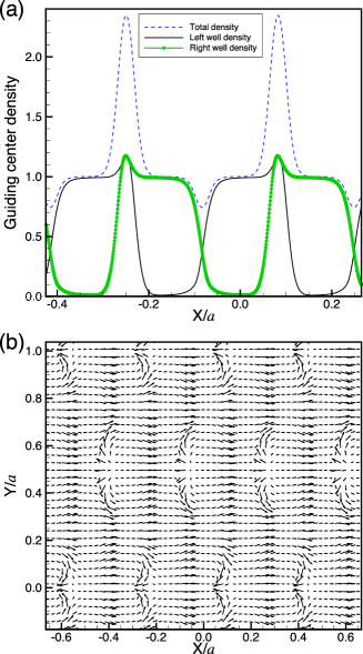
Figure 4: Representation of the soliton crystal at $d/\ell=1.2$, $\widetilde{t}=0.01$ and $\nu=9.1.$The distance between two solitons in a channel is $a.$ (a) Guiding-center densities $\rho_{RR}\left(x,y\right),\rho_{LL}\left(x,y\right)$ and $\rho\left(x,y\right)=\rho_{RR}\left(x,y\right)+\rho_{LL}\left(x,y\right)$ at $y=0$; (b) pseudospin texture showing the solitons localized in the channels.

III Field-theoretic model

We use two different approaches to compute the energy gap due to the excitation of soliton-antisoliton pairs. The first one is a field-theoretic calculation valid in the limit of slowly varying pseudospin textures. It is explained in this section. The second one is a microscopic approach where the energy of one soliton is computed from that of a crystal of solitons by removing the soliton-soliton interaction. We call this method the supercell approach. In principle, this second method is not restricted to small gradient of the pseudospin texture and includes terms neglected in the field-theoretic model. We expect it to be more accurate than the field-theoretic approach.

In the field-theoretic approach, we evaluate the energy to create a pseudospin soliton by making a long-wavelength expansion of certain terms in the Hartree-Fock Hamiltonian. We follow the procedure developped in details in Ref. macdobible, . To keep the discussion as brief as possible, we give here only the main results of this model. Full details are provided in the appendix.

There are three main contributions to the energy needed to create a pseudospin texture in a LCR. Since in the ground state the in-plane pseudospin component in a LCR is fully polarized along $S_{x}$, adding a pseudospin texture has a tunnel energy cost when $t\neq 0$ because of the interaction of the texture with the other channels. A second contribution comes from the interlayer exchange interaction which is responsible for the pseudospin stiffness $\rho_{s}$. As we mentioned above, the exchange interaction favors pseudospin textures that vary slowly in space. A third contribution must be considered in our model in order to get agreement with the microscopic approach. It is the Coulomb interaction between different portions of the soliton in a channel. This interaction favors large solitons.

If the coherent channels are oriented along $y$ and are considered as effectively one-dimensional, then the energy cost to make a pseudospin texture on top of the ground state where all pseudospins point in the $x$ direction in each channel is

$$\delta E=\int dy\left[\frac{1}{2}\rho_{s}\left(\frac{\partial\varphi(y)}{\partial y}\right)^{2}-T\left[\cos\varphi(y)-1\right]\right].$$ (12)

where $\varphi(y)$ in the azimuthal angle of the pseudospins. Eq. (12) is valid if we ignore the third contribution mentionned above. The parameters $\rho_{s}$ and $T$ are the effective stiffness and tunneling parameters. These parameters depend on the precise shape of the LCR’s as well as on the interaction between pseudospins of different channels. In the appendix, we derive a microscopic expression for each of these parameters in terms of the order parameters of the CSP. We show that the effective stiffness is given by

$$\rho_{s}=\frac{-1}{16\pi^{2}\ell^{2}}\left(\frac{e^{2}}{\kappa\ell}\right)\int dq_{x}\lvert\Omega(q_{x})\rvert^{2}\,\,\left.\frac{d^{2}X_{R,L}(N,N;\mathbf{q})}{dq_{y}^{2}}\right|_{q_{y}\rightarrow 0},$$ (13)

where

$$\Omega(q_{x})=\xi\sum_{G_{x}}\left\langle\rho_{N}^{x}(G_{x})\right\rangle\frac{\sin\left[\left(G_{x}-q_{x}\right)\xi/4\right]}{\left(G_{x}-q_{x}\right)\xi/4},$$ (14)

is a form factor that takes into account the shape of the channel centered at $x=0$. Also, $\xi$ is the interstripe distance in the CSP, $G_{x}=2\pi n/\xi$ with $n=0,\pm 1,\pm 2,...$ and $\left\langle\rho_{N}^{x}(G_{x})\right\rangle=\mathrm{Re}\left[\left\langle\rho_{N}^{R,L}(G_{x})\right\rangle\right].$ If we define the parameter $\widetilde{G}_{x}=4\pi n/\xi$ and

$$J_{\bot}\left(\mathbf{q}\right)=-X_{R,L}\left(N,N;\mathbf{q}\right),$$ (15)

then the parameter $T$ can be written as

$$T=\frac{1}{2\pi\ell^{2}}\left(\frac{e^{2}}{\kappa\ell}\right)\left[\widetilde{t}\Omega(q_{x}=0)-\frac{1}{\xi}\sum_{\widetilde{G}_{x}}J_{\bot}\left(\widetilde{G}_{x},0\right)\lvert\Omega(G_{x})\rvert^{2}+\frac{1}{2}\frac{1}{L_{x}}\sum_{q_{x}}J_{\bot}\left(q_{x},0\right)\left|\Omega\left(q_{x}\right)\right|^{2}\right].$$ (16)

The second and third terms in Eq. (16) come from the fact that, because of the pseudospin stiffness, there is an energy cost to rotate the pseudospins in one channel when the pseudospins in the other channels remain fixed in their ground state position. The contribution of these two terms increases the effective tunneling strength $T$. Since the energy cost to create a pseudospin soliton is given by $E_{s}=8\sqrt{\rho_{s}T}$ we see that this second term keeps $E_{s}$ finite even when $\widetilde{t}=0$.

In this field-theoretic model, the energy to create an antisoliton is the same as that needed to create a soliton and the charge gap is simply given by

$$\Delta=16\sqrt{\rho_{s}T}.$$ (17)

From the energy functional of Eq. (12), we get that the static solution that minimizes the energy must satisfy the sine-Gordon equation

$$\frac{\partial^{2}\varphi(y)}{\partial y^{2}}=\frac{T}{\rho_{s}}\sin\varphi(y).$$ (18)

The sine-Gordon (or kink) soliton is a solution of this equation. It is given by

$$\varphi(y)=4\tan^{-1}\left[e^{\sqrt[-]{\frac{T}{\rho_{s}}}y}\right].$$ (19)

The length of the soliton can be defined as

$$L_{s}=\sqrt{\frac{\rho_{s}}{T}}.$$ (20)

With the energy functional of Eq. (12), we find numerically that both $\rho_{s}$ and $T$ decrease rapidly with $d$ but the size of the soliton $L_{s}$ decreases with increasing $d$. This behavior is opposite to what we obtain in the microscopic calculation where the soliton size increases with $d$. As we mentionned above, it is necessary to include the Coulomb interaction between different part of the solitons in order to get the soliton size to increase with $d$. This leads to the term (full details are given in the appendix)

$$\delta E_{Coul}=\frac{\ell^{2}}{32\pi^{2}}\int dy\int dy^{\prime}\frac{d\varphi\left(y\right)}{dy}V_{\text{\emph{eff}}}\left(y-y^{\prime}\right)\frac{d\varphi\left(y^{\prime}\right)}{dy^{\prime}}$$ (21)

Inclusion of this term in in the energy functional introduces a nonlocal non-linear term in the differential equation for the soliton and the resulting equation is very difficult to solve. Following S. Ghosh and R. Rajaramanghosh who use a similar procedure in their calculation of the energy of CP³ skyrmions in bilayers, we make the following approximation. We insert a pseudospin texture $\varphi(y)=4\tan^{-1}\left[e^{-y/L_{s}^{\ast}}\right]$ into the total energy functional including the Coulomb integral and evaluate is as a function of $L_{s}^{\ast}$. We then minimize the total energy with respect to the length $L_{s}^{\ast}$ to obtain the energy and length of the soliton. In this way, we find a soliton length that increases with $d$ as in the microscopic approach. The procedure is described in details in the appendix.

IV The supercell microscopic Hartree-Fock method

Let $\varepsilon_{CSP}$ be the energy per electron in the CSP at $\nu=4N+1$ and magnetic field $B_{0}$ in units of $e^{2}/\kappa\ell_{0}$. If the number of electrons is kept constant and the magnetic field is decreased (to $B_{1}$) or increased (to $B_{2}$) such that the filling factor becomes $\nu=4N\pm\widetilde{\nu}$, then a finite density $n_{qp}=\left|\widetilde{\nu}-1\right|/2\pi\ell_{1,2}^{2}$ of quasiparticles (solitons for $\widetilde{\nu}>1$ and antisolitons for $\widetilde{\nu}<1$) are created in the CSP. At zero temperature, we expect these quasiparticles to crystallize and to be localized in the LCR’s of the CSP. In the limit where only one quasiparticle is created ($\widetilde{\nu}\rightarrow 1$), we can define the quasiparticle energy as

$$E_{qp}^{\pm}=\lim_{N_{qp}\rightarrow 1}\frac{\nu}{\left|\widetilde{\nu}-1\right|}\left[\varepsilon_{SC}\left(\frac{e^{2}}{\kappa\ell_{1,2}}\right)-\varepsilon_{CSP}\left(\frac{e^{2}}{\kappa\ell_{0}}\right)\right],$$ (22)

where $\varepsilon_{SC}$ is the energy per electron in the soliton crystal (SC) in units of $e^{2}/\kappa\ell$ with $N_{qp}$ solitons and $E_{qp}^{+}\left(E_{qp}^{-}\right)$ is the energy to create one soliton (antisoliton).

The quasiparticle energy defined in this way, with the number of electrons kept constant, is refered to as the “proper” quasiparticle energy by Morf and HalperinMorfHalperin . Other definitions are also possible. For example, the “gross” quasiparticle energies (or chemical potentials) are defined by

$$\mu^{+} = E\left(N_{e}=N_{\phi}+1\right)-E\left(N_{e}=N_{\phi}\right),$$ (23)

$$\mu^{-} = E\left(N_{e}=N_{\phi}\right)-E\left(N_{e}=N_{\phi}-1\right),$$ (24)

where $N_{\phi}$ is the degeneracy of the Landau levels at a magnetic field $B_{0}$ such that $\nu=4N+1.$ The energy $E\left(N_{\phi}\right)$ is the total energy of the CSP, and $E\left(N_{\phi}\pm 1\right)$ is the total energy of the CSP with one more (less) particle in the form of a soliton (antisoliton). In this case, the magnetic field is kept constant while the number of particles changes. At zero temperature, this is precisely the definition of the chemical potentials at filling factors slightly above or below $\nu=4N+1.$

The different definitions of the the quasiparticle energies lead to different numerical values. As discussed by MacDonald and Girvinmacdoquasip , however, the numerical value of the gap, $\Delta,$ is the same for both definitions so that we can write

$$\Delta=\mu^{+}-\mu^{-}=E_{qp}^{+}+E_{qp}^{-}.$$ (25)

With the formalism described in Sec. II, we can easily compute the Hartree-Fock energy of a crystal of solitons located in the coherent channels of the bilayer. That is, we can compute $\varepsilon_{SC}$, find $E_{qp}^{\pm}$ and then the energy gap. However, there are several difficulties with this method that we address in this paper. The first one is that the limit $n_{qp}\rightarrow 1$ cannot be achieved numerically since that would require infinite matrices in the equation of motion for the single-particle Green’s function. In this work, we have succeeded in computing $\varepsilon_{SC}$ at filling as small as $\widetilde{\nu}=1\pm 0.02.$ The second difficulty is that, when a finite density of quasiparticles is present, $\varepsilon_{SC}$ includes the interaction energy between quasiparticles. This interaction energy must be computed and removed from $\varepsilon_{SC}.$ A third difficulty is related to the size of the solitons (antisolitons). In Sec. III, we saw that the soliton size becomes very large when the tunneling energy $\widetilde{t}\rightarrow 0$ or when $d$ is large. In this case the size of the soliton is not given by Eq. (20) but is limited by the lattice constant of the soliton crystal. The quasiparticle energy, then, cannot be computed reliably when the tunneling term is too small or the interlayer distance too big.

We now describe in more details our evaluation of $E_{qp}^{\pm}.$ To avoid computing numerically the energy of the antisoliton crystal as well as that of the soliton crystal, we use the particle-hole symmetry of the Hamiltonian around $\nu=4N+1$ to relate the energies of the two crystals with the same filling of quasiparticles. We define state $0$ as the CSP at $\nu=4N+1$, state $1$ as the soliton crystal at $\nu_{1}=4N+\widetilde{\nu}_{1}$ and state $2$ as the crystal of antisolitons at $\nu_{2}=4N+\widetilde{\nu}_{2}$. The filling factors $\widetilde{\nu}_{2}=2-\widetilde{\nu}_{1}$ so that the lattice constants $a_{1}$ and $a_{2}$ of the two crystals are related by $\ell_{1}/a_{1}=\ell_{2}/a_{2}$. The Hartree-Fock energy per electron of the three states are given by Eq. (II) which we rewrite here as

$$\frac{E_{m}}{N_{e}}=\left[\left(\frac{\widetilde{\nu}_{m}}{\nu_{m}}\right)\varepsilon_{m}\left(\widetilde{\nu}_{m}\right)+\frac{1}{\nu_{m}}\Lambda\left(\widetilde{\nu}_{m}\right)\right]\left(\frac{e^{2}}{\kappa\ell_{m}}\right).$$ (26)

We have defined

$$\varepsilon_{m}\left(\widetilde{\nu}_{m}\right)=-\frac{2\widetilde{t}}{\widetilde{\nu}_{m}}\mathrm{Re}\left[\langle\rho_{N}^{R,L}(0)\rangle_{m}\right]$$ (27)

$$+\frac{1}{2\widetilde{\nu}_{m}}\sum_{i,j}\sum_{\mathbf{G}\neq 0}H_{i,j}\left(N,N,\mathbf{G}\right)\left\langle\rho_{N}^{i,i}\left(-\mathbf{G}\right)\right\rangle_{m}\left\langle\rho_{N}^{j,j}\left(\mathbf{G}\right)\right\rangle_{m}$$

$$-\frac{1}{2\widetilde{\nu}_{m}}\sum_{i,j}\sum_{\mathbf{G}}X_{i,j}\left(N,N,\mathbf{G}\right)\left\langle\rho_{N}^{i,j}\left(-\mathbf{G}\right)\right\rangle_{m}\left\langle\rho_{N}^{j,i}\left(\mathbf{G}\right)\right\rangle_{m},$$

which is the energy per electron in the partially filled level. The last term in Eq. (26) is the interaction energy with the filled level with

$$\Lambda\left(\widetilde{\nu}_{i}\right)=-2\Lambda_{1}-\Lambda_{2}\widetilde{\nu}_{i},$$ (28)

where

$$\Lambda_{1} = \sum_{n<N}\sum_{n^{\prime}<N}X_{R,R}\left(n,n^{\prime},0\right),$$ (29)

$$\Lambda_{2} = \sum_{n<N}X_{i,i}\left(n,N,0\right).$$ (30)

From Eqs. (23) and (24), it is easy to see that the cyclotron and Zeeman energies do not contribute to the transport gap $\Delta$ and so can be ignored in Eq. (26). This is also true of the filled levels since their contribution to the quasiparticle energies are given by

$$\left(E_{qp}^{+}\right)_{f.l.} = \lim_{N_{qp}\rightarrow 1}\frac{\nu_{1}}{\left|\widetilde{\nu}_{1}-1\right|}\left(\frac{e^{2}}{\kappa\ell_{1}}\right)\frac{1}{\nu_{1}}\Lambda\left(\widetilde{\nu}_{1}\right)$$

$$-\lim_{N_{qp}\rightarrow 1}\frac{\nu_{1}}{\left|\widetilde{\nu}_{1}-1\right|}\frac{1}{4N+1}\Lambda\left(1\right)\left(\frac{e^{2}}{\kappa\ell_{0}}\right)$$

$$= \left(\frac{e^{2}}{\kappa\ell_{0}}\right)\left[\frac{1}{2}\Lambda_{2}+3\Lambda_{1}\right],$$

and

$$\left(E_{qp}^{-}\right)_{f.l.} = \lim_{N_{qp}\rightarrow 1}\frac{\nu_{2}}{\left|\widetilde{\nu}_{2}-1\right|}\left(\frac{e^{2}}{\kappa\ell_{2}}\right)\frac{1}{\nu_{2}}\Lambda\left(\widetilde{\nu}_{2}\right)$$

$$-\left(\frac{e^{2}}{\kappa\ell_{0}}\right)\lim_{N_{qp}\rightarrow 1}\frac{\nu_{2}}{\left|\widetilde{\nu}_{2}-1\right|}\frac{1}{4N+1}\Lambda\left(1\right)$$

$$= -\left(\frac{e^{2}}{\kappa\ell_{0}}\right)\left[\frac{1}{2}\Lambda_{2}+3\Lambda_{1}\right],$$

so that $\left(E_{qp}^{+}\right)_{f.l.}+\left(E_{qp}^{-}\right)_{f.l.}=0.$ In deriving these two equations, we have used

$$\left(\frac{e^{2}}{\kappa\ell_{1}}\right)=\left(\frac{e^{2}}{\kappa\ell_{0}}\right)\sqrt{\frac{\nu_{0}}{\nu_{1}}}.$$ (33)

From the electron-hole symmetry, we get

$$\varepsilon_{2}=\left(\frac{\widetilde{\nu}_{1}}{2-\widetilde{\nu}_{1}}\right)\left[\varepsilon_{1}+\left(\frac{\widetilde{\nu}_{1}-1}{\widetilde{\nu}_{1}}\right)X\left(0\right)\right],$$ (34)

where

$$X\left(0\right)=X_{R,R}\left(N,N,\mathbf{0}\right).$$ (35)

Note that Eq. (34) is exact only in the limit where $N_{qp}\rightarrow 1$ because the inter-well Hartree and Fock interactions contained in $\varepsilon_{m}$ depend on the ratio $d/\ell$ and we have $d/\ell_{1}\neq d/\ell_{2}$.

Combining all results, we have for the energy gap

$$\Delta = \lim_{\Delta\nu\rightarrow 0}\frac{1}{\Delta\nu}\widetilde{\nu}_{1}\left[\sqrt{\frac{\nu_{0}}{\nu_{1}}}+\sqrt{\frac{\nu_{0}}{\nu_{2}}}\right]\varepsilon_{1}\left(\frac{e^{2}}{\kappa\ell_{0}}\right)$$ (37)

$$+\lim_{\Delta\nu\rightarrow 0}\frac{1}{\Delta\nu}\left[\sqrt{\frac{\nu_{0}}{\nu_{2}}}X\left(0\right)-2\widetilde{\varepsilon}_{CSP}\right]\left(\frac{e^{2}}{\kappa\ell_{0}}\right),$$

where we have defined

$$\varepsilon_{CSP}=\frac{1}{4N+1}\widetilde{\varepsilon}_{CSP}.$$ (38)

Simplifying, we get finally

$$\Delta=\lim_{\Delta\nu\rightarrow 0}\left[2\frac{\widetilde{\nu}_{1}}{\Delta\nu}\varepsilon_{1}-\frac{2}{\Delta\nu}\widetilde{\varepsilon}_{CSP}+X\left(0\right)\right]\left(\frac{e^{2}}{\kappa\ell_{0}}\right).$$ (39)

We remark that the change in the magnetic length $\ell$ due to the change in the magnetic field makes no contribution to the energy gap. We could have ignored it in Eq. (26). In fact, the gap defined using Eq. (22) and taking $e^{2}/\kappa\ell_{i}=e^{2}/\kappa\ell_{0}$ is the so-called neutral energy gapmacdoquasip and it is equal to the other two gaps that we introduced in this section.

Eq. (39) can also be written as

$$\Delta=2E_{qp}^{+}+\left[2\varepsilon_{CSP}+X\left(0\right)\right]\left(\frac{e^{2}}{\kappa\ell_{0}}\right).$$ (40)

In the lowest Landau level, the energy gap at $\nu=1$ is due to the excitation of a bimeron-antibimeron pair and the energy per electron in the UCS is $\varepsilon_{UCS}\left(d\right)=\left[-\widetilde{t}-\frac{1}{4}\left[X\left(0\right)+\widetilde{X}_{d}\left(0\right)\right]\right]$ where $\widetilde{X}\left(0\right)=X_{R,L}\left(N,N,\mathbf{0}\right)$. Eq. (40) can then be written, for this special case, as

$$\Delta=2E_{qp}^{+}+2\left[\varepsilon_{UCS}\left(d\right)-\varepsilon_{UCS}\left(d=0,t=0\right)\right]\left(\frac{e^{2}}{\kappa\ell_{0}}\right),$$ (41)

which is just the form we used in Ref. breybimeron, .

V Interaction between quasiparticles

With the simplifications introduced in the preceding section, the energy $\varepsilon_{SC}$ that enters Eq. (22) and Eq. (39) is given by

$$\varepsilon_{SC}=-\frac{2\widetilde{t}}{\widetilde{\nu}}\mathrm{Re}\left[\langle\rho^{R,L}(0)\rangle\right]$$ (42)

$$+\frac{1}{2\widetilde{\nu}}\sum_{i,j}\sum_{\mathbf{G}\neq 0}H_{i,j}\left(\mathbf{G}\right)\left\langle\rho^{i,i}\left(-\mathbf{G}\right)\right\rangle\left\langle\rho^{j,j}\left(\mathbf{G}\right)\right\rangle$$

$$-\frac{1}{2\widetilde{\nu}}\sum_{i,j}\sum_{\mathbf{G}}X_{i,j}\left(\mathbf{G}\right)\left\langle\rho^{i,j}\left(-\mathbf{G}\right)\right\rangle\left\langle\rho^{j,i}\left(\mathbf{G}\right)\right\rangle,$$

where, to simplify the notation, we have left implicit the index $N$ of the Landau level. The soliton crystal is a superposition of a CSP with order parameters $\left\{\left\langle\alpha^{i,j}\left(\mathbf{G}\right)\right\rangle\right\}$ (computed at $\nu=4N+1$) and a pure soliton crystal (PSC) with order parameters $\left\{\left\langle\beta^{i,j}\left(\mathbf{G}\right)\right\rangle\right\}$ such that

$$\left\langle\rho^{i,j}\left(\mathbf{G}\right)\right\rangle=\left\langle\alpha^{i,j}\left(\mathbf{G}\right)\right\rangle+\left\langle\beta^{i,j}\left(\mathbf{G}\right)\right\rangle.$$ (43)

If we insert this decomposition into Eq. (42), we find

$$\varepsilon_{SC}=\varepsilon_{CSP}\left(\widetilde{\nu}\right)+\varepsilon_{CSP-PSC}+\varepsilon_{PSC},$$ (44)

where

$$\varepsilon_{CSP}\left(\widetilde{\nu}\right)=-\frac{2\widetilde{t}}{\widetilde{\nu}}\mathrm{Re}\left[\langle\alpha^{R,L}(0)\rangle\right]$$ (45)

$$+\frac{1}{2\widetilde{\nu}}\sum_{i,j}\sum_{\mathbf{G}\neq 0}H_{i,j}\left(\mathbf{G}\right)\left\langle\alpha^{i,i}\left(-\mathbf{G}\right)\right\rangle\left\langle\alpha^{j,j}\left(\mathbf{G}\right)\right\rangle$$

$$-\frac{1}{2\widetilde{\nu}}\sum_{i,j}\sum_{\mathbf{G}}X_{i,j}\left(\mathbf{G}\right)\left\langle\alpha^{i,j}\left(-\mathbf{G}\right)\right\rangle\left\langle\alpha^{j,i}\left(\mathbf{G}\right)\right\rangle$$

is the energy per electron of the CSP (i.e. $\varepsilon_{CSP}\left(\widetilde{\nu}\right)=\frac{1}{\widetilde{\nu}}\widetilde{\varepsilon}_{CSP}$),

$$\varepsilon_{PSC}=-\frac{2\widetilde{t}}{\widetilde{\nu}}\mathrm{Re}\left[\langle\beta^{R,L}(0)\rangle\right]$$ (46)

$$+\frac{1}{2\widetilde{\nu}}\sum_{i,j}\sum_{\mathbf{G}\neq 0}H_{i,j}\left(\mathbf{G}\right)\left\langle\beta^{i,i}\left(-\mathbf{G}\right)\right\rangle\left\langle\beta^{j,j}\left(\mathbf{G}\right)\right\rangle$$

$$-\frac{1}{2\widetilde{\nu}}\sum_{i,j}\sum_{\mathbf{G}}X_{i,j}\left(\mathbf{G}\right)\left\langle\beta^{i,j}\left(-\mathbf{G}\right)\right\rangle\left\langle\beta^{j,i}\left(\mathbf{G}\right)\right\rangle$$

is the energy per electron of the PSC and

$$\varepsilon_{CSP-PSC}=$$ (47)

$$+\frac{1}{\widetilde{\nu}}\sum_{i,j}\sum_{\mathbf{G}\neq 0}H_{i,j}\left(\mathbf{G}\right)\left\langle\alpha^{i,i}\left(-\mathbf{G}\right)\right\rangle\left\langle\beta^{j,j}\left(\mathbf{G}\right)\right\rangle$$

$$-\frac{1}{\widetilde{\nu}}\sum_{i,j}\sum_{\mathbf{G}}X_{i,j}\left(\mathbf{G}\right)\left\langle\alpha^{i,j}\left(-\mathbf{G}\right)\right\rangle\left\langle\beta^{j,i}\left(\mathbf{G}\right)\right\rangle$$

is the interaction energy (per electron) between the CSP and the PSC.

The contribution $\varepsilon_{PSC}$ causes problem because it contains not only the energy to create the $N_{qp}$ solitons but also the interaction energy between the solitons. This interaction energy goes away in the limit $\Delta\nu\rightarrow 0$. As we said, however, we cannot go to arbitrarily small $\Delta\nu$ numerically because solving the equation of motion for the single-particle Green’s function then involves diagonalizing very large matrices. We must then find a way to remove the interaction energy in $\varepsilon_{PSC}$. Two methods can be used. The first one is to replace $\varepsilon_{PSC}$ by $\varepsilon_{PSC}-\varepsilon_{int}$ where $\varepsilon_{int}$ is the Madelung energy of the crystal of charged quasiparticles, assuming the quasiparticles to be point particlesbreybimeron . We refer to this method as the “Madelung” method. In the limit $\Delta\nu\rightarrow 0$, the quasiparticles are very far apart and, if they have an isotropic charge distribution, it is a reasonable approximation. In the second method, which we refer to as the “form factor” method, we completely replace $\varepsilon_{PSC}\left(\left\{\left\langle\beta^{i,j}\left(\mathbf{G}\right)\right\rangle\right\}\right)$ by the energy $N_{qp}\varepsilon_{PSC}\left(\left\{\left\langle\beta_{qp}^{i,j}\left(\mathbf{q}\right)\right\rangle\right\}\right)$ where $\varepsilon_{PSC}\left(\left\{\left\langle\beta_{qp}^{i,j}\left(\mathbf{q}\right)\right\rangle\right\}\right)$ is the energy per electron of a “crystal” of only one quasiparticle. In the case of solitons, which are quite extended and highly anisotropic objects it is necessary to use this second approach.

To evaluate $\varepsilon_{PSC}\left(\left\{\left\langle\beta_{qp}^{i,j}\left(\mathbf{q}\right)\right\rangle\right\}\right)$, we make use of the fact that, when the quasiparticles are very far apart (limit $\widetilde{\nu}\rightarrow 1$) so that there is no overlap of the density or spin texture due to different quasiparticles, then we may think of the order parameters in real space as given by

$$\left\langle\beta^{i,j}\left(\mathbf{r}\right)\right\rangle=\sum_{\mathbf{R}}h_{i,j}\left(\mathbf{r-R}\right),$$ (48)

where $\mathbf{R}$ is a lattice site. We know that

$$\left\langle\beta^{i,j}\left(\mathbf{r}\right)\right\rangle=\frac{1}{V}\sum_{\mathbf{G}}\left\langle\beta^{i,j}\left(\mathbf{G}\right)\right\rangle e^{-i\mathbf{G}\cdot\mathbf{r}},$$ (49)

but it is not possible to get $h_{i,j}\left(\mathbf{r}\right)$ from this equation. We must make an approximation. Since we work in the low-density limit for the quasiparticles, it is a good approximation to assume that for a “crystal” of one quasiparticle

$$\left\langle\beta^{i,j}\left(\mathbf{r}\right)\right\rangle_{qp}=\left\{\begin{array}[]{ccc}\frac{1}{V}\sum_{\mathbf{G}}\left\langle\beta^{i,j}\left(\mathbf{G}\right)\right\rangle e^{-i\mathbf{G}\cdot\mathbf{r}},&\mathrm{if}&\mathbf{r}\in v_{c}\\ 0,&\mathrm{if}&\mathbf{r\notin}v_{c}\end{array}\right.,$$ (50)

where $v_{c}$ is the volume of the unit cell centered at $\mathbf{r}=0.$ Fourier transforming Eq. (50), we have

$$\left\langle\beta^{i,j}\left(\mathbf{q}\right)\right\rangle_{qp} = \int_{V}d\mathbf{r}e^{i\mathbf{q}\cdot\mathbf{r}}\left\langle\beta^{i,j}\left(\mathbf{r}\right)\right\rangle_{qp}$$

$$= \frac{1}{N_{qp}}\sum_{\mathbf{G}}\left\langle\beta^{i,j}\left(\mathbf{G}\right)\right\rangle\Lambda\left(\mathbf{q}-\mathbf{G}\right)\mathbf{,}$$

where the form factor

$$\Lambda\left(\mathbf{q}-\mathbf{G}\right)=\frac{1}{v_{c}}\int_{v_{c}}d\mathbf{r}e^{i\mathbf{q}\cdot\mathbf{r}}e^{-i\mathbf{G}\cdot\mathbf{r}},$$ (52)

depends on the shape of the unit cell of the soliton crystal.

It now remains to compute the Hartree-Fock energy corresponding to the density and pseudospin textures given by the $\left\langle\beta_{i,j}\left(\mathbf{q}\right)\right\rangle_{qp}$’s. The energy is still given by an equation similar to Eq. (46) where the summation $\frac{1}{2\widetilde{\nu}}\sum_{\mathbf{G}}$ is now replaced by $\frac{1}{2\widetilde{\nu}}\sum_{\mathbf{q}}$. To go from the sum to the integral, we use

$$\frac{1}{2\widetilde{\nu}}\sum_{\mathbf{q}}\left(\ldots\right) \rightarrow \frac{S}{2\widetilde{\nu}}\int\frac{d\mathbf{q}}{\left(2\pi\right)^{2}}\left(\ldots\right)$$

$$\rightarrow \frac{2\pi\widetilde{N}_{e}}{2\widetilde{\nu}^{2}}\int\frac{d\mathbf{q}\ell^{2}}{\left(2\pi\right)^{2}}\left(\ldots\right).$$

Aso, because $\left\langle\beta^{i,j}\left(\mathbf{0}\right)\right\rangle_{qp}\sim 1/N_{\varphi}$, we introduce a new field $\Theta^{i,j}\left(\mathbf{q}\right)$ by the definition

$$\Theta^{i,j}\left(\mathbf{q}\right)=N_{\varphi}\left\langle\beta^{i,j}\left(\mathbf{q}\right)\right\rangle_{qp}.$$ (54)

With this last definition, we have

$$N_{qp}\varepsilon_{PSC}\left(\left\{\left\langle\beta_{qp}^{i,j}\left(\mathbf{q}\right)\right\rangle\right\}\right)$$

$$= \frac{\pi\Delta\nu}{\widetilde{\nu}}\sum_{i,j}\int\frac{d\mathbf{q}\ell^{2}}{\left(2\pi\right)^{2}}H_{i,j}\left(\mathbf{q}\right)\Theta^{i,i}\left(-\mathbf{q}\right)\Theta^{j,j}\left(\mathbf{q}\right)$$

$$-\frac{\pi\Delta\nu}{\widetilde{\nu}}\sum_{i,j}\int\frac{d\mathbf{q}\ell^{2}}{\left(2\pi\right)^{2}}X_{i,j}\left(\mathbf{q}\right)\Theta^{i,j}\left(-\mathbf{q}\right)\Theta^{j,i}\left(\mathbf{q}\right).$$

As a test of our “form factor” method, we have computed the energy gap due to the creation of bimeron-antibimeron pairs at $\nu=1$ in the lowest Landau level $N=0.$ Figure 5 shows the energy gap computed from a triangular lattice of bimerons at $\nu=1.02$ and $\widetilde{t}=0.0025.$ In this case, the Madelung and form factor methods give identical results at small interlayer distances while the Madelung method slighlty overestimates the energy gap at higher distances. The difference between the two approches at large $d$ is due to the fact that the charge density profile of the bimeron becomes more and more anisotropic as $d$ increases. Also, the Coulomb interaction is stronger between point particles than between extended particles so that the Madelung approach overestimates the gap energy.

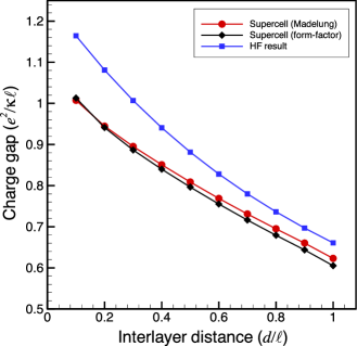
Figure 5: The energy gap due to the excitation of a bimeron-antibimeron pair $\nu=1$ computed using the form factor or the Madelung method and compared with the Hartree-Fock energy gap to the excitation of an electron-hole pair.

To check the convergence of the supercell approach as the lattice constant gets very large, we show in Fig. 6 the energy gap of the UCS at $\nu=1$ computed at different values of $\nu$ from a crystal of bimerons. The different curves in this figure are for different values of the tunneling strength. The real gap of the system is, of course, defined for $\nu\rightarrow 1.$ We see that the gap converges more rapidly to its $\nu\rightarrow 1$ value when the tunneling is stronger. This is understandable since the size of a bimeron decreases when $\widetilde{t}$ increases and, for sufficiently strong $\widetilde{t}$, this size is independent of the lattice constant even at relatively high $\nu$. For smaller $\widetilde{t}$ the gap converges to its $\nu\rightarrow 1$ value, but only at lower filling $\nu$. In the application of the supercell technique to the soliton gap in the next section, we will use the form factor method to remove the interaction energy. As we have just shown, this method is more appropriate in the case where the quasiparticle is highly anisotropic in shape.

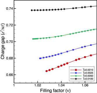
Figure 6: Energy gap of the UCS at $\nu=1$ computed by the supercell approach using the form factor method. The different curves are for different values of the tunneling strength $\widetilde{t}.$

VI Numerical results

We now discuss our numerical results for the energy gap of the CSP. Our calculations are done in Landau level $N=2$ around $\nu=9$ using the form factor method. Figures 7(a)-(c) contain our main results. Differents gaps are plotted as a function of the interlayer distance for tunnelings (a) $\widetilde{t}=0.007;$ (b) $\widetilde{t}=0.01$; and (c) $\widetilde{t}=0.02$. The filled line is $\Delta_{UCS},$ the energy needed to create an ordinary electron-hole pair from the coherent liquid state at $\nu=9.$ At $\nu=9$, the liquid state is unstable for $d>d_{1}$ where the coherent striped state is the ground state. The Hartree-Fock gap represented by the curve with the filled squares is given by the energy to create an electron-hole pair in a coherent channel (see Fig. 2 where this gap is defined). The other curves give the energy gap calculated in the supercell method for different filling factors $\nu$ and the energy gap calculated with the field-theoretic approach explained in the appendix.

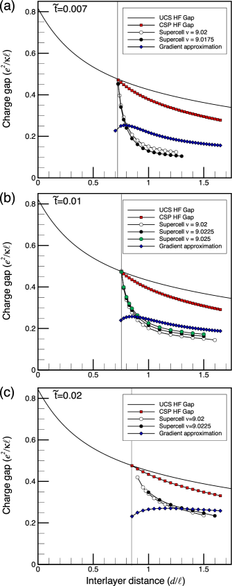
Figure 7: Different energy gaps in the UCS and CSP calculated as a function of the interlayer distance $d/\ell$ and for different values of the tunneling parameter. For the supercell method, the gap is evaluated at different filling factors to show the convergence of the results to the true gap at $\nu=9$. The gradient approximation refers to the field-theoretic method.

From Fig. 7, it is clear that, in the CSP, the energy needed to create a soliton-antisoliton pair is smaller than that needed to create an electron-hole pair for typical experimental values of the tunneling parameter $\widetilde{t}$. The transport gap is thus determined by the creation of these topological excitations (as it was the case for skyrmions in quantum Hall ferromagnet at $\nu=1$ or with bimerons in bilayer quantum Hall systems).breybimeron Figures 7(a)-(c) show a rapid decrease of the energy gap near the transition between the coherent liquid and the CSP that should be observable experimentally. The curves corresponding to different filling factors show that the convergence of the supercell method is quite good near the liquid-CSP transition but slow at larger values of interlayer distances. This slow convergence is due to the fact that the size of the soliton increases with interlayer distance as shown in Fig. 8 and the shape of the soliton is then restricted by the lattice constant as we explained previously. As $d/\ell$ increases, it becomes necessary to go to lower filling factors to achieve convergence, something we cannot do numerically. In any case, the soliton gap is always lower than the Hartree-Fock gap at higher values of $d/\ell$ since our approach overestimates the energy gap. Increasing $\widetilde{t}$ decreases the size of the solitons, however, so that it is possible to achieve better convergence by increasing the value of the tunneling parameter $\widetilde{t}$. This is seen by comparing Fig. 7 (a), (b) and (c). Notice also that, for smaller solitons, the soliton gap is closer to the Hartree-Fock result, as expected.

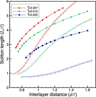
Figure 8: Soliton size calculated with the supercell (filled symbols) and field-theoretic (empty symbols) methods as a function of the interlayer distance at $\nu=9.02.$ In the supercell approach the size of the soliton is found by fitting the $y$ dependence of the phase in a channel with $\varphi(y)=4\tan^{-1}\left[e^{-y/L_{s}}\right].$

We also show in Fig. 7 the gap calculated with the field-theoretic method (see Eq. (17)). This gap has the same qualitative behavior with interlayer distance, except at small $d$ near the phase transition. It is larger than the gap calculated in the microscopic approach. As we explain in the appendix, the field-theoretic result is incorrect at small $d$ or large $\widetilde{t}$ (fig. 7(c)) where the stripes are not fully developped. At large $d$, we cannot say how different the two gaps (macroscopic and field-theoretic) are because the gap found in the microscopic approach has not yet converged at the lowest filling factor we can achieve.

In the field-theoretic method, the soliton size, $L_{s}^{\ast},$ is obtained by the procedure outlined in Sec. III . When the Coulomb interaction between parts of the soliton is properly included, we find numerically that $L_{s}^{\ast}$ increases with $d$ as in the supercell calculation. Both approaches give the same trend for the soliton length. The detailed behaviour with $d/\ell$ is quite different, however. Cearly, the field-theoretic calculation does not capture all the subtleties of the We recall that, as the interlayer distance increases, the width of the LCR’s becomes smaller. The behavior of the soliton size may be understood as arising from the Coulomb energy, which favors spreading the charge of the soliton. Our results are plotted in Fig. 8. In this figure, we see that the supercell and field-theoretic results do not match for large $\widetilde{t}$. This is again due to the fact that the stripes are not fully formed at large $\widetilde{t}$ so that the expression of Eq. (A.3) for the topological charge is not correct. As expected, Fig. 8 shows that the soliton size decreases with $\widetilde{t}$.

We have neglected quantum fluctuations in our calculation. These fluctuations increases in importance as $d/\ell$ increases. They renormalize the pseudospin stiffness and will probably also change the size of the solitons and the quantitative values of the energy gaps. Inclusion of these fluctuations is, however, beyond the scope of this paper.

VII Conclusion

We have computed the energy gap due to the creation of a soliton-antisoliton pair in the linearly coherent channel of the coherent striped phase found in higher Landau levels in a bilayer quantum Hall system. We have computed this gap using a microscopic unrestricted Hartree-Fock approach as well as a field-theoretic approach valid in the limit of slowly varying pseudospin texture. With both methods, we find that the this energy gap is lower in energy than the Hartree-Fock gap due to the creation of an electron-hole pair in a coherent channel (a single spin flip) so that solitonic excitations must play an important role in the transport properties of the coherent striped phase.

VIII Acknowledgements

This work was supported by a research grant (for R.C.) and graduate research grants (for C. B. D.) both from the Natural Sciences and Engineering Research Council of Canada (NSERC). H.A.F. acknowledges the support of NSF through Grant No. DMR-0454699.

*

Appendix A Microscopic expressions for the parameters of the field-theoretic model

In this appendix we present the details of the derivation of the microscopic expressions for the parameters $\rho_{s}$ and $T$ used in the field-theoretic model of Sec. III. We drop the Landau level index $N$ here since all order parameters are to evaluated in the partially filled level $N$. We begin by defining the pseudospin density operators

$$\rho(\mathbf{q}) =\rho^{R,R}(\mathbf{q})+\rho^{L,L}(\mathbf{q}),$$ (56)

$$\rho_{z}(\mathbf{q}) =\frac{1}{2}\left[\rho^{R,R}(\mathbf{q})-\rho^{L,L}(\mathbf{q})\right],$$ (57)

$$\rho_{x}(\mathbf{q}) =\frac{1}{2}\left[\rho^{R,L}(\mathbf{q})+\rho^{L,R}(\mathbf{q})\right],$$ (58)

$$\rho_{y}(\mathbf{q}) =\frac{1}{2i}\left[\rho^{R,L}(\mathbf{q})-\rho^{L,R}(\mathbf{q})\right].$$ (59)

The total Hartree-Fock energy of the electrons in the partially filled level for an unbiased bilayer can be written as

$$E_{HF}=\varepsilon\left(\frac{e^{2}}{\kappa\ell}\right),$$ (60)

where

$$\varepsilon = -2N_{\phi}\widetilde{t}\left\langle\rho_{x}\left(0\right)\right\rangle$$

$$+\frac{1}{4}N_{\phi}\sum_{\mathbf{q}}\Upsilon\left(\mathbf{q}\right)\left\langle\rho\left(-\mathbf{q}\right)\right\rangle\left\langle\rho\left(\mathbf{q}\right)\right\rangle$$

$$+N_{\phi}\sum_{\mathbf{q}}J_{z}\left(\mathbf{q}\right)\left\langle\rho_{z}\left(-\mathbf{q}\right)\right\rangle\left\langle\rho_{z}\left(\mathbf{q}\right)\right\rangle$$

$$+N_{\phi}\sum_{\mathbf{q}}J_{\bot}\left(\mathbf{q}\right)[\left\langle\rho_{x}\left(-\mathbf{q}\right)\right\rangle\left\langle\rho_{x}\left(\mathbf{q}\right)\right\rangle$$

$$\qquad+\left\langle\rho_{y}\left(-\mathbf{q}\right)\right\rangle\left\langle\rho_{y}\left(\mathbf{q}\right)\right\rangle].$$

We have introduced the interactions

$$J_{z}\left(\mathbf{q}\right)=H_{R,R}\left(\mathbf{q}\right)-H_{R,L}\left(\mathbf{q}\right)-X_{R,R}\left(\mathbf{q}\right),$$ (62)

$$\Upsilon\left(\mathbf{q}\right)=H_{R,R}\left(\mathbf{q}\right)+H_{R,L}\left(\mathbf{q}\right)-X_{R,R}\left(\mathbf{q}\right),$$ (63)

and

$$J_{\bot}\left(\mathbf{q}\right)=-X_{R,L}\left(\mathbf{q}\right).$$ (64)

In Eq. (A), $H_{R,R}\left(0\right)=H_{R,L}\left(0\right)=0$ because of the interaction between the 2DEG and the positive background of the donors.

We now introduce a unitless and unitary pseudospin field $S_{\alpha}(\mathbf{r})$, with $\alpha=x,y,z$ related to the guiding center density operators in the pseudospin formalism by the relation

$$S_{\alpha}(\mathbf{r})=4\pi\ell^{2}N_{\phi}\left\langle\rho_{\alpha}(\mathbf{r})\right\rangle,$$ (65)

and a projectednote1 electron density by the relation

$$n(\mathbf{r})=N_{\phi}\left\langle\rho(\mathbf{r})\right\rangle.$$ (66)

Using the definition of the pseudospin operators $S_{\alpha}({r})$ and taking the Fourier transform of Eq. (A), we have

$$\varepsilon = \frac{-\widetilde{t}}{2\pi\ell^{2}}\int d\mathbf{r}S_{x}(\mathbf{r})$$

$$+\frac{1}{8\pi\ell^{2}}\int d\mathbf{r}\int d\mathbf{r}^{\prime}J_{\perp}(\mathbf{r}-\mathbf{r}^{\prime})\mathbf{S}_{\perp}(\mathbf{r})\cdot\mathbf{S}_{\perp}(\mathbf{r}^{\prime})$$

$$+\frac{1}{8\pi\ell^{2}}\int d\mathbf{r}\int d\mathbf{r}^{\prime}S_{z}(\mathbf{r})J_{z}(\mathbf{r}-\mathbf{r}^{\prime})S_{z}(\mathbf{r}^{\prime})$$

$$+\frac{\pi\ell^{2}}{2}\int d\mathbf{r}\int d\mathbf{r}^{\prime}n(\mathbf{r})\Upsilon(\mathbf{r}-\mathbf{r}^{\prime})n(\mathbf{r}^{\prime}).$$

Writing $S_{\alpha}(\mathbf{r})$ in spherical coordinates, it is easy to describe the CSP ground state as

$$S_{x}(\mathbf{r})_{CSP} =\sin\theta(x),$$ (68)

$$S_{y}(\mathbf{r})_{CSP} =0,$$ (69)

$$S_{z}(\mathbf{r})_{CSP} =\cos\theta(x),$$ (70)

while the density $\left\langle n(\mathbf{r})\right\rangle=cst$ is uniform. For a state where there is a spin texture only in the channel centered at $x=0$ (channel $0$) while the other channels remain in their CSP ground state configuration (we recall that $\xi$ is the interstripe distance), we write

$$S_{x}(\mathbf{r})=\begin{cases}\sin\theta(x)\cos\varphi(y),&\text{if $|x|\leq\frac{\xi}{4}$},\\ \sin\theta(x),&\text{if $|x|>\frac{\xi}{4}$},\end{cases}$$ (71)

$$S_{y}(\mathbf{r})=\begin{cases}\sin\theta(x)\sin\varphi(y),&\text{if $|x|\leq\frac{\xi}{4}$},\\ 0,&\text{if $|x|>\frac{\xi}{4},$}\end{cases}$$ (72)

$$S_{z}(\mathbf{r})=S_{z}(\mathbf{r})_{CSP},$$ (73)

$$n(\mathbf{r})=n(\mathbf{r})_{CSP}+\delta n(\mathbf{r}).$$ (74)

In these equations, $\theta(x)$ is given by its value in the CSP. Defining

$$J_{i,j}(y-y^{\prime})\equiv\int_{C_{i}}dx\int_{C_{j}}dx^{\prime}J_{\perp}(\mathbf{r}-\mathbf{r^{\prime}})\sin\theta(x)\sin\theta(x^{\prime}),$$ (75)

where $C_{i}$ corresponds to the $i$-th channel of width $\xi/2$ centered at $x_{i}$ and $\int_{C_{i}}=\int_{x_{i}-\xi/4}^{x_{i}+\xi/4}$ , it is easy to show that the energy difference between the this last state and the CSP ground state i.e. the energy to create one soliton in a channel is given by

$$\begin{split}\delta\varepsilon&=\frac{-\widetilde{t}}{2\pi\ell^{2}}\int_{C_{0}}dx\sin\theta(x)\int dy\left[\cos\varphi(y)-1\right]\\ +&\frac{1}{4\pi\ell^{2}}\sum_{i\neq 0}\int dy\int dy^{\prime}J_{i,0}(y-y^{\prime})\left[\cos\varphi(y^{\prime})-1\right]\\ +&\frac{1}{8\pi\ell^{2}}\int dy\int dy^{\prime}J_{0,0}(y-y^{\prime})\left[\cos(\varphi(y)-\varphi(y^{\prime}))-1\right]\\ &+\frac{\pi\ell^{2}}{2}\int d\mathbf{r}\int d\mathbf{r}^{\prime}\delta n(\mathbf{r})\Upsilon(\mathbf{r}-\mathbf{r}^{\prime})\delta n(\mathbf{r}^{\prime})\\ &+\pi\ell^{2}\int d\mathbf{r}\int d\mathbf{r}^{\prime}\delta n(\mathbf{r})\Upsilon(\mathbf{r}-\mathbf{r}^{\prime})n(\mathbf{r}^{\prime})_{CSP}.\end{split}$$ (76)

The first two terms contribute to the effective tunnelling term $T$ while the third term is directly related to the pseudospin stiffness of the system. The fourth term takes into account the Coulomb interaction between different parts of the soliton and the last term is the interaction between the charge of the soliton and that of the CSP. In an antisoliton, this fifth contribution would have exactly the same value but with opposite sign so that this last term does not contribute to the transport gap.

A.1 Calculation of the pseudospin stiffness $\rho_{s}$

To extract the pseudospin stiffness from the third term of Eq. (76), we make a long-wavelength expansion of the $\cos(\varphi(y)-\varphi(y^{\prime}))-1$ term. This expansion is possible if the pseudospin texture varies slowly in comparison with $J_{0,0}(y)$. We get

$$\frac{1}{8\pi\ell^{2}}\int dy\int dy^{\prime}J_{0,0}(y-y^{\prime})\left[\cos(\varphi(y)-\varphi(y^{\prime}))-1\right]$$

$$=-\frac{1}{16\pi\ell^{2}}\left[\int dy^{\prime}\,\,y^{\prime}{}^{2}J_{0,0}(y^{\prime})\right]\int dy\left(\frac{d\varphi(y)}{dy}\right)^{2}.$$ (77)

Comparing this last result with Eq. (12), we see that

$$\rho_{s}=-\frac{1}{8\pi\ell^{2}}\int dy\,\,y^{2}J_{0,0}(y).$$ (78)

The pseudospin stiffness can be written, more explicitely as

$$\rho_{s} = -\frac{1}{8\pi\ell^{2}}\int dy\,\,y^{2}\frac{1}{L_{x}L_{y}}\sum_{\mathbf{q}}J_{\perp}(\mathbf{q})e^{iq_{y}y}$$

$$\times\int_{C_{0}}dx\int_{C_{0}}dx^{\prime}\sin\theta(x)\sin\theta(x^{\prime})e^{iq_{x}(x-x^{\prime})},$$

with $L_{x}$ and $L_{y}$ the length and width of the sample. This allows the integrals over $x$ and $x^{\prime}$ to be totally decoupled. In fact, defining the form factor

$$\Omega(q_{x}) = \int_{C_{0}}dx\sin\theta(x)e^{iq_{x}x}$$

$$= \xi\sum_{G_{x}}\langle\rho_{x}(G_{x})\rangle\frac{\sin\left[(G_{x}-q_{x})\xi/4\right]}{(G_{x}-q_{x})\xi/4},$$

we can write

$$\rho_{s}=\frac{1}{16\pi^{2}\ell^{2}}\int dq_{x}\lvert\Omega(q_{x})\rvert^{2}\,\,\left.\frac{d^{2}J_{\perp}(\mathbf{q})}{dq_{y}^{2}}\right|_{q_{y}\rightarrow 0}.$$ (81)

The form factor $\Omega(q_{x})$ takes into account the influence of the shape of the charge modulation along the $x$ axis in the CSP phase on the effective pseudospin stiffness in the one dimensional sine-Gordon model.

A.2 Calculation of the tunneling parameter $T$

The effective tunnel coupling $T$ can be extracted from the first two terms of Eq. (76). The first term renormalizes the tunnel coupling in the 1D effective theory, taking into account that interlayer coherence exists only in the LCR’s. This first term is simply

$$\frac{-\widetilde{t}}{2\pi\ell^{2}}\Omega(0)\int dy\left[\cos\varphi(y)-1\right].$$ (82)

The second contribution to the effective tunnel coupling comes from the exchange energy between channel $0$ (where a pseudospin texture was created) and the other channels. In these other channels, the in-plane pseudospin component is totally polarized along the $\mathbf{x}$ direction and the exchange interaction between channel $i$ and channel $0$ favors a configuration in channel $0$ where the pseudospin is also polarized along $+\mathbf{x}$, just like the simple tunnel coupling $\widetilde{t}$. In other words, there is an energy cost, even in the absence of tunneling, to make a rotation of the pseudospins in one channel because of the interaction with the pseudospins in the other channels.

It is possible to extract a simple form for this coupling from the second term of Eq. (76) since

$$\sum_{i\neq 0}\int dyJ_{i,0}(y) = \frac{1}{L_{x}}\sum_{i\neq 0}\sum_{q_{x}}J_{\perp}(q_{x},0)|\Omega(q_{x})|^{2}e^{iq_{x}(x_{i}-x_{0})}$$ (83)

$$= \frac{1}{L_{x}}\sum_{i}\sum_{q_{x}}J_{\perp}(q_{x},0)|\Omega(q_{x})|^{2}e^{iq_{x}(x_{i}-x_{0})}$$

$$-\frac{1}{L_{x}}\sum_{q_{x}}J_{\perp}(q_{x},0)|\Omega(q_{x})|^{2},$$

with $x_{n}-x_{0}=n\xi/2$ the center-to-center distance between channels $n$ and $0$. Because there is a sum over the channels, the sum on the wave-vectors $q_{x}$ reduces to a sum over the reciprocal lattice vectors of a 1D lattice of lattice constant $\xi/2$, noted $\widetilde{G}_{x}$, and

$$\begin{split}&\frac{1}{2}\sum_{i\neq 0}\int dy\int dy^{\prime}J_{i,0}(y-y^{\prime})\left[\cos\varphi(y^{\prime})-1\right]\\ &=\frac{1}{\xi}\sum_{\widetilde{G}_{x}}J_{\perp}(\widetilde{G}_{x},0)|\Omega(\widetilde{G}_{x})|^{2}-\frac{1}{2}\frac{1}{L_{x}}\sum_{q_{x}}J_{\perp}(q_{x},0)|\Omega(q_{x})|^{2}.\end{split}$$ (84)

Combining the two terms, we find

$$T = \frac{1}{2\pi\ell^{2}}\left[\Omega(0)\widetilde{t}-\frac{1}{\xi}\sum_{\widetilde{G}_{x}}J_{\perp}(\widetilde{G}_{x})\left|\Omega\left(\widetilde{G}_{x}\right)\right|^{2}\right.$$

$$\left.+\frac{1}{2}\frac{1}{L_{x}}\sum_{q_{x}}J_{\bot}\left(q_{x},0\right)\left|\Omega\left(q_{x}\right)\right|^{2}\right].$$

A.3 Sine-Gordon soliton and the Coulomb energy

If we combine the tunneling and exchange terms, we find that the energy cost to make one soliton localized in a channel of the CSP is given by Eq. (12). As we mentionned in Sec. III, the static solution that minimizes this energy functional is the sine-Gordon (or kink) soliton $\varphi(y)=4\tan^{-1}\left[e^{\sqrt[-]{\frac{T}{\rho_{s}}}y}\right].$

We now add to Eq. (12) the Coulomb interaction energy between different parts of the soliton

$$\delta E_{Coul}=\frac{\pi\ell^{2}}{2}\int d\mathbf{r}\int d\mathbf{r}^{\prime}\delta n\left(\mathbf{r}\right)\Upsilon\left(\mathbf{r}-\mathbf{r}^{\prime}\right)\delta n\left(\mathbf{r}^{\prime}\right).$$ (86)

To relate $\delta n(\mathbf{r}^{\prime})$ to the angles $\theta$ and $\varphi$, we use the definition of the topological charge density given in Eq. (11). We assume that, in the one-soliton state, only $\varphi\left(y\right)$ changes along a channel and that $\theta\left(\mathbf{r}\right)$ is given by its value in the CSP. We have

$$\delta n\left(\mathbf{r}\right) = -\frac{1}{4\pi}\nabla\varphi\left(\mathbf{r}\right)\times\left(\nabla\cos\theta\left(\mathbf{r}\right)\right)\cdot\widehat{\mathbf{z}}$$

$$= \frac{1}{4\pi}\frac{d\varphi\left(y\right)}{dy}\frac{d}{dx}\cos\theta\left(x\right).$$

At this point, we must remark that if we use the sine-Gordon solution in Eq. (A.3) and integrate the projected density $\delta n\left(\mathbf{r}\right)$ in a channel, we find $\int_{-\xi/4}^{+\xi/4}dx\int_{-\infty}^{+\infty}dy\delta n\left(\mathbf{r}\right)=1$ only if $\cos\theta\left(x\right)$ varies from $-1$ to $+1$ in the channel i.e. only in the limit or large interlayer distances where the stripes are fully developped. In consequence, we do not expect our field-theoretic model to be valid near the transition between the UCS and the CSP.

We insert Eq. (A.3) into Eq. (86), and define the form factor (for a channel centered at $x=0$)

$$A\left(q_{x}\right) = \int_{C_{0}}dxe^{-iq_{x}x}\frac{d}{dx}\cos\theta\left(x\right)$$

$$= i\xi\sum_{G_{x}}\left\langle\rho_{z}\left(G_{x}\right)\right\rangle G_{x}\frac{\sin\left(q_{x}-G_{x}\right)\xi/4}{\left(q_{x}-G_{x}\right)\xi/4},$$

and the effective interaction $V_{\text{\emph{eff}}}\left(y-y^{\prime}\right)$ in a channel

$$V_{\text{\emph{eff}}}\left(y-y^{\prime}\right)=\frac{1}{S}\sum_{\mathbf{q}}\left|A\left(q_{x}\right)\right|^{2}\Upsilon\left(\mathbf{q}\right)e^{iq_{y}\left(y-y^{\prime}\right)}.$$ (89)

We then find for the Coulomb interaction

$$\delta E_{\text{\emph{Coul}}}=\frac{\ell^{2}}{32\pi^{2}}\int dy\int dy^{\prime}\frac{d\varphi\left(y\right)}{dy}V_{\text{\emph{eff}}}\left(y-y^{\prime}\right)\frac{d\varphi\left(y^{\prime}\right)}{dy^{\prime}}.$$ (90)

If we add the contribution $\delta E_{\text{\emph{Coul}}}$ to Eq. (12) and minimize the energy with respect to $\varphi\left(y\right)$, we find that it introduces a nonlocal term to the sine-Gordon equation. The resulting equation is then very difficult to solve. To get an approximation for the Coulomb energy, we decided to proceed in the following way. We take, as a trial solution, the kink soliton

$$\varphi(y)=4\tan^{-1}\left[e^{-y/L_{s}^{\ast}}\right],$$ (91)

where $L_{s}^{\ast}$ is the width of the soliton. The Coulomb energy is then

$$\delta E_{\text{\emph{Coul}}}\left(L_{s}^{\ast}\right)=\frac{\pi\ell^{2}}{32\pi^{2}}\int d\mathbf{q}\left|A\left(q_{x}\right)\right|^{2}\Upsilon\left(q\right)\text{sech}^{2}\left(\frac{\pi q_{y}L_{s}^{\ast}}{2}\right).$$ (92)

The total energy for the soliton is

$$E=4\frac{\rho_{s}}{L_{s}^{\ast}}+4TL_{s}^{\ast}+\delta E_{\text{\emph{Coul}}}\left(L_{s}^{\ast}\right).$$ (93)

We find $L_{s}^{\ast}$ by minimizing numerically the total energy $E$. In our numerical calculation, we use $\Upsilon\left(\mathbf{q}\right)=H_{N}\left(\mathbf{q}\right)$ instead of Eq. (63). This is also the interaction considered in similar calculationsmacdobible ,rajaraman . The use of Eq. (63) leads to non-physical results.

References

• (1) A. A. Koulakov, M. M. Fogler and B. I. Shklovskii, Phys. Rev. Lett. 76, 499 (1996); M. M. Fogler, A. A. Koulakov, and B. I. Shklovskii, Phys. Rev. B 54, 1853 (1996); R. Moessner and J.T. Chalker, Phys. Rev. B 54, 5006 (1996); M. M. Fogler and A. A. Koulakov, Phys. Rev. B 55, 9326 (1997). For a review of the bubble and stripe phases in higher Landau levels, see M. Fogler in High Magnetic Fields: Applications in Condensed Matter Physics and Spectroscopy, ed. by C. Berthier, L.-P. Levy, G. Martinez (Springer-Verlag, Berlin), 99 (2002).
• (2) M. P. Lilly, K. B. Cooper, J. P. Eisenstein, L. N. Pfeiffer and K. W. West, Phys. Rev. Lett. 82, 394 (1999); R. R. Du, D. C. Tsui, H. L. Stormer, L. N. Pfeiffer, K. W. Baldwin and K. W. West, Solid State Comm. 109, 389 (1999).
• (3) L. Brey and H. A. Fertig, Phys. Rev. B 62, 10268 (2000).
• (4) D. Bouchiha, M. Sc. Thesis, Université de Sherbrooke, 2002.
• (5) R. Côté and H. A. Fertig, Phys. Rev. B 65, 085321 (2002).
• (6) R. Côté, H. A. Fertig, J. Bourassa, and D. Bouchiha, Phys. Rev. B 66, 205315 (2002).
• (7) Daw-Wei Wang, Eugene Demler, and S. Das Sarma, Phys. Rev. B 68, 165303 (2003).
• (8) E. Demler, D.-W. Wang, S. Das Sarma, and B. I. Halperin, Solid State Comm. 123, 243 (2002).
• (9) Emiliano Papa, John Schliemann, A. H. MacDonald, and Matthew P. A. Fisher, Phys. Rev. B 67, 115330 (2003).
• (10) R. Côté and A. H. MacDonald, Phys. Rev. Lett. 65, 2662 (1990); R. Côté and A. H. MacDonald, Phys. Rev. B 44, 8759 (1991).
• (11) K. Moon, H. Mori, Kun Yang, S. M. Girvin, A. H. MacDonald, L. Zheng, D. Yoshioka, and Shou-Cheng Zhang, Phys. Rev. B 51, 5138 (1995).
• (12) R. Rajaraman, Solitons and Instantons, (North-Holland, New York, 1989).
• (13) L. Brey, H. A. Fertig, R. Côté, and A. H. MacDonald, Phys. Rev. B 54, 16888 (1996).
• (14) R. Côté, C. B. Doiron, J. Bourassa, and H. A. Fertig, Phys. Rev. B 68, 155327 (2003).
• (15) S. Ghosh and R. Rajaraman, Phys. Rev. B 63, 035304 (2000).
• (16) R. Morf and B. I. Halperin, Phys. Rev. B 33, 2221 (1986).
• (17) A. H. MacDonald and S. M. Girvin, Phys. Rev. B 34, 5639 (1986).
• (18) Lynn Bonsall and A. A. Maradudin, Phys. Rev. B 15, 1959 (1977).
• (19) The relation between the true density and the guiding center density is given by $n(\mathbf{q})=N_{\phi}\rho(\mathbf{q})F(\mathbf{q})$ where $F(\mathbf{q})$ is a form factor that depends on the Landau level index. In this work we use call $n(\mathbf{q})=N_{\phi}\rho(\mathbf{q})$ the projected density.