⁽¹⁾ Presently at ]Laboratoire de Physique Statistique, CNRS & École Normale Sup rieure, 24 rue Lhomond, 75005 Paris, France

Intermittency of velocity time increments in turbulence.

Abstract

We analyze the statistics of turbulent velocity fluctuations in the time domain. Three cases are computed numerically and compared: (i) the time traces of Lagrangian fluid particles in a (3D) turbulent flow (referred to as the dynamic case); (ii) the time evolution of tracers advected by a frozen turbulent field (the static case), and (iii) the evolution in time of the velocity recorded at a fixed location in an evolving Eulerian velocity field, as it would be measured by a local probe (referred to as the virtual probe case). We observe that the static case and the virtual probe cases share many properties with Eulerian velocity statistics. The dynamic (Lagrangian) case is clearly different; it bears the signature of the global dynamics of the flow.

One of the distinctive feature of turbulence is the development of extremely high fluctuation level at small scales. The probability density functions (PDFs) of velocity increments are stretched at small scales, while they are almost Gaussian at large scale where energy is fed into the flow Frisch . This evolution is traditionally referred to as “intermittency” in turbulence studies. Numerous studies have been devoted to the study of intermittency in the spatial domain, analyzing velocity differences between two points separated by a variable distance $\mathbf{r}$. For instance, it is now well established that when the velocity increments are computed along the distance $\mathbf{r}$, the longitudinal velocity increments are skewed and the structure functions have universal relative scaling exponents in the inertial range Arneodo ; SheLev ; Cas , related to the graininess of the dissipation. When the increments are related to changes in the velocity component perpendicular to the distance $\mathbf{r}$, the corresponding transverse structure functions display a different scaling, related to the spatial distribution of vorticity Transverse . In contrast, there has been much fewer studies of intermittency in the time domain, i.e., related to changes in time of the velocity field. Two cases are of particular importance: The Lagrangian one, which pertains to the fluctuations in time of the velocity of marked fluid particles, and the Eulerian one, where one considers the variations in time of the velocity measured at a fixed location in the flow. We consider of course the case where turbulence develops in the absence of a mean flow, otherwise Taylor’s hypothesis trivially reduces the second case to a spatial measurement Tayloc . Eulerian time fluctuations are different because one expects, after Tennekes original suggestion Tenn , that sweeping (the random advection by large scale motion) plays an important role. In practice, Eulerian intermittency in time is relevant for stationary bodies exposed to turbulent flow conditions (atmospheric ones, for instance). Lagrangian intermittency, on the other hand, has strong implications for processes such as mixing LagMix , combustion LagCombustion , or cloud formation LagRain . Lagrangian data has recently been made available in numerical simulations PopeYeung ; Biferale and experimental measurements Voth98 ; OttMann ; MordantPinton1 . One rather unexpected feature is the observation of long-time correlations in the Lagrangian dynamics MordantPinton2 . It has been incorporated in recent stochastic models of Lagrangian acceleration Sawford ; Reynolds — see also Arin for a recent review. However, the full modelization of Lagrangian velocity fluctuations is still in progress. Lagrangian statistics are often computed from the advection of particles in a frozen Eulerian field (to minimize computing overhead). We have thus decided to compare this pseudo-Lagrangian statistics to that of pure Lagrangian and Eulerian time fluctuations.

We study the problem numerically. We first compute the velocity changes of fluid particles that are advected by a frozen 3D Eulerian velocity field; that is, we consider a single snapshot of a converged turbulent flow, and use it to advect fluid particles in this frozen Eulerian field — we call this the static case. Then we compute the velocity variations of true Lagrangian particles, a situation in which the Eulerian flow is also evolved in time according to the Navier-Stokes equations — this case is called the dynamic case. Finally, we record the time evolution of the Eulerian velocity at fixed locations of the computation domain, as it would be measured by virtual velocity probes. We then perform a comparative study of the intermittency characteristics of the three velocity time signals. We show that the statistics of time velocity increments depends on the situation considered: the static case and the virtual probes display intermittency features that are reminiscent of Eulerian velocity statistics; the former has multifractal spectra identical to the ones measured for 3D Eulerian turbulence Kestener , while the later coincides with traditional longitudinal Eulerian velocity increments statistics Frisch . The dynamic case, which is a true Lagrangian measurement, displays significantly more intermittent features.

The Navier-Stokes equations are integrated in a $256^{3}$ cubic domain of size $2\pi$ by a parallel distributed memory pseudo-spectral solver, using a second-order (in time) leap-frog scheme. The large-scale kinetic-energy forcing is adjusted at each time step by scaling the amplitudes of modes $1.5\leq k<2.5$ uniformly (phases are left to fluctuate freely), so as to compensate exactly the losses due to eddy dissipation in the kinetic-energy budget levkoud . The Reynolds number based on the Taylor microscale is $R_{\lambda}=140$. The velocity root mean square is 0.1214 m/s, the mean dissipation rate is $\epsilon=0.0011{\rm m}^{2}/{\rm s}^{3}$ and the kinematic viscosity is $\nu=1.5\;10^{-4}{\rm m}^{2}/{\rm s}$. The particles trajectories are resolved in time by a second-order Runge-Kutta scheme, and interpolated using cubic spline functions. In the dynamic case, a set of 10,000 particles, uniformly distributed in the cube at initial time, are followed for a duration of approximatively 7$T_{L}$. Here, as in ChevPRL , $T_{L}$ is defined for each signal as the time scale above which the velocity statistics is Gaussian (the second order cumulant has reached the Gaussian value $\pi^{2}/8$). For the static case, 10,000 trajectories have been integrated over approximatively 3$T_{L}$. Finally, 32,768 virtual probes have been used to get the time variation of the Eulerian field at a fixed location; in this case the records are 10 $T_{L}$ long. We label $v_{D,i}(t)$ the Lagrangian velocity of one component (in cartesian coordinates) of particle number $i$ in the 3D Eulerian time-evolving flow (dynamic case), $v_{S,i}(t)$ one component of the velocity advected by the static Eulerian flow (static case) and $v_{T,i}(t)$ the time evolution of one component of an Eulerian velocity probe.

In Fig. 1 we show the power spectral densities $\langle|\hat{v}_{S}(\omega)|^{2}\rangle$, $\langle|\hat{v}_{D}(\omega)|^{2}\rangle$ and $\langle|\hat{v}_{T}(\omega)|^{2}\rangle$ vs. $\omega T_{L}$ in a logarithmic representation, where $\hat{v}$ means Fourier transform of $v$, for the static, the dynamic cases (averaged over the number of tracked particles) and for the virtual fixed probes (averaged over the number of probes). One observes for all cases, a scaling behavior on a small range of scales. We show in the inset the values of the corresponding power law exponent determined from the local logarithmic slope of the spectra. The dynamic Lagrangian velocity spectrum has an $\omega^{-2}$ inertial range spectrum, as expected from Kolmogorov similiraty arguments TenLum , and in agreement with previous experimental and numerical observations MordantPinton1 . The spectrum of the time variation of the Eulerian velocity field (as recorded by the virtual probes) shows a clear $-5/3$ scaling exponent, characteristic of Eulerian data Frisch . This is in good agreement with Tennekes sweeping argument Tenn ; Vergass : the characteristic velocity fluctuations at scale $\ell$ is the standard deviation of the flow velocity $v_{\rm rms}=\sqrt{\langle|v_{S}|^{2}\rangle}$ rather than the Kolmogorov one $v_{\ell}=(\epsilon\ell)^{1/3}$. As a result, a time-scale increment $\tau$ corresponds to a length $\ell=v_{\rm rms}\tau$, so that the scaling of the increments is in fact Eulerian. In addition, this effect produces a larger inertial range because the dissipative time scale is $T_{L}R_{\lambda}^{-3/2}$ for the Eulerian time data, while it is $T_{L}R_{\lambda}^{-1}$ for the dynamic Lagrangian data. Fig. 1 then shows that the data in the static case also follow a $-5/3$ scaling law, closer to the Eulerian behavior than to the Lagrangian one. This result has also been found in a similar study using Kinematic Simulations of turbulence Vass , a situation in which the Eulerian velocity field is monofractal, i.e. not intermittent. Let us mention that since inertial range statistics are likely to be independent on the Reynolds number, we consider the behavior of our estimators in the inertial range (i.e, power spectra in Fig. 1 and cumulants of magnitude in Fig. 2) as characteristics of fully developed turbulence — despite the moderate Reynolds number value of our DNS ($R_{\lambda}\simeq 140$).

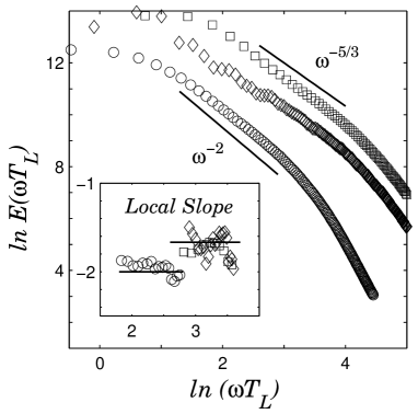
Figure 1: Power spectral density $E(\omega T_{L})$ of one component of the velocity of tracer particles in the static ($\square$) and dynamic ($\circ$) cases, and for the virtual Eulerian probes ($\diamond$). Spectra have been shifted vertically for clarity. The local slopes of these spectra are plotted in the inset.

We now seek to quantify the intermittency features. This is usually done via the analysis of the scaling behavior of velocity structure functions Frisch $S(p,\tau)=\langle|\delta_{\tau}v|^{p}\rangle=\langle|v(t+\tau)-v(t)|^{p}\rangle\sim\tau^{\zeta_{p}}$, where the average is computed over all accessible times $t$ and over all recorded time series. Note that we use the absolute value of velocity increments in the definition of the structure functions in Eq. (1) since the statistics that are studied are symmetric under the transformation $\delta_{\tau}v\rightarrow-\delta_{\tau}v$ : velocity increment statistics are not skewed. However, as advocated in DelMuz for Eulerian velocity data analysis, the magnitude cumulant analysis provides a more reliable alternative to the structure function method. The relationship between the moments of $|\delta_{\tau}v|$ and the cumulants $C_{n}(\tau)$ of $\ln|\delta_{\tau}v|$ reads

$$\langle|\delta_{\tau}v|^{p}\rangle=\exp\left(\sum_{n=1}^{\infty}C_{n}(\tau)\frac{p^{n}}{n!}\right)\mbox{ .}$$ (1)

Previous studies MordantPinton1 ; MordantPinton2 ; ChevPRL have shown that intermittency is suitably described for small $p$ using a log-normal statistical framework corresponding to a quadratic $\zeta_{p}$ spectrum :

$$\zeta_{p}=c_{1}p-c_{2}\frac{p^{2}}{2}\mbox{ ,}$$ (2)

where the parameters $c_{1}$ and $c_{2}$ can be extracted from the time scale behavior of the first two cumulants $C_{1}(\tau)$ and $C_{2}(\tau)$. In Eulerian context, the analysis of longitudinal velocity increments in the inertial range has shown that $C_{2}^{E}(\ell)=-c_{2}^{E}\ln(\ell/L)$, where $\ell$ is a spatial scale and $L$ the decorrelation length, with a universal intermittency coefficient $c_{2}^{E}\approx 0.025$ DelMuz ; Cas .

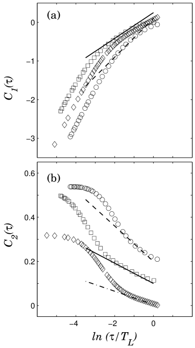
Figure 2: Cumulants of velocity magnitude for the static ($\square$) and dynamic ($\circ$) cases, and for the virtual Eulerian probes ($\diamond$). (a) $C_{1}^{S,D,T}(\tau)$ vs. $\ln(\tau/T_{L})$; the solid and dashed lines correspond to the slopes $c_{1}^{S,T}=1/3$ and $c_{1}^{D}=1/2$ respectively; for the sake of clarity, we have substracted $\langle\ln|\delta_{T_{L}}v|\rangle$. (b) $C_{2}^{S,D,T}(\tau)$ vs. $\ln(\tau/T_{L})$; the solid, dashed-dotted and dashed lines correspond to the slopes $c_{2}^{S}=0.046$, $c_{2}^{T}=0.03$ and $c_{2}^{D}=0.08$ respectively; we have subtracted $\mbox{Var}[\ln|\delta_{T_{L}}v|]=\pi^{2}/8$ and also shifted the upper curves by 0.1 and 0.2 for clarity.

We report in Fig. 2 the results of a comparative analysis of the cumulants $C_{1}^{S,D,T}(\tau)$ and $C_{2}^{S,D,T}(\tau)$. The profile of $C_{1}^{D}(\tau)$ as a function of $\ln(\tau/T_{L})$ is significantly curved, a feature that has also been observed on experimental data of Lagrangian velocity structure functions MordantPinton1 . This departure from scaling is a signature of (i) the pollution of the inertial range by dissipative (finite Reynolds number) effects as studied in ChevPRL and (ii) the non universal and/or anisotropic behavior of the turbulent flow at scales of the order of the integral time scale $\sim T_{L}$. In Fig. 2(a), we have indicated by a dashed line the scaling behavior $C_{1}^{D}(\tau)=c_{1}^{D}\ln(\tau/T_{L})$, with $c_{1}^{D}=\langle h\rangle\simeq 1/2$ corresponding to a $(\omega T_{L})^{-2}$ scaling region in the power spectrum (we recall that $h\simeq 1/2$ corresponds to the most probable velocity scaling exponent in a multifractal analysis of Lagrangian intermittency MordantPinton2 ; ChevPRL ). In contrast, the first order cumulant for the static case and for the Eulerian velocity time variations is better represented by $C_{1}^{S,T}(\tau)=c_{1}^{S,T}\ln(\tau/T_{L})$, with $c_{1}^{S,T}=\langle h\rangle\approx 1/3$, as indicated by the continuous line in Fig. 2(a). Again, this value is consistent with the $(\omega T_{L})^{-5/3}$ power spectrum behavior observed in Fig. 1. As it is also the case for Eulerian fields DelMuz ; Cas , the second order cumulants — Fig. 2(b) — has a logarithmic behavior in the inertial range, $C_{2}^{S,D,T}(\tau)=-c_{2}^{S,D,T}\ln(\tau/T_{L})$. In the dynamic case, we get $c_{2}^{D}\simeq 0.08$, in good agreement with previous experimental data ChevPRL and numerical simulations Biferale .

The static case and the Eulerian time probes follow the same behavior, with $c_{2}^{S}\simeq 0.046$ and $c_{2}^{T}\simeq 0.03$. The first value is in good agreement with the recent estimate of the intermittency coefficient $c_{2}^{E,3D}=0.049$ of a numerical 3D Eulerian velocity field Kestener . Note that $c_{2}^{E,3D}$ is significantly larger than the value $c_{2}^{E}\simeq 0.025$ computed for longitudinal velocity increments, to which one should compare the estimate of the intermittency coefficient $c_{2}^{T}$ of the time variations of the Eulerian longitudinal velocity component. As a technical but important point, we stress that the values of $c_{2}$ reported here are not computed from a linear regression fit in the $C_{2}(\tau)$ curves (due to the narrowness of the inertial range) but as a result of the mutifractal description of the entire range of scales, dissipative domain included, as detailed in ChevPRL .

We thus conclude that the static and Eulerian intermittencies in time have identical statistics to respectively 3D and 1D Eulerian fields, while the true dynamic (Lagrangian) case is clearly different and more intermittent. This is confirmed in Fig. 3 where the more familiar structure function exponents $\zeta_{p}$ are compared. Note that in order to be able to compare Eulerian and Lagrangian data, all exponents are computed using the second order structure function as a reference (extended self-similarity (ESS) ansatz ESS ) in order (i) to overcome the observed bending of the structure functions when plotted versus the time scale in a logarithmic representation (as already noticed in Fig. 2(a) for the first cumulant $C_{1}(\tau)$), and (ii) to give a clear picture of intermittency effects responsible for departure from a linear behavior (i.e. $\zeta_{p}^{D}\neq p/2$ and $\zeta_{p}^{T},\zeta_{p}^{S}\neq p/3$). Thus, in this representation, each $\zeta_{q}$ spectrum must be compared to the monofractal Kolmogorov’s prediction $\zeta_{p}=p/2$.

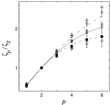
Figure 3: Structure function exponent $\zeta_{p}/\zeta_{2}$ vs. $p$ as computed for the static case ($\square$), the dynamic ($\circ$) case and the Eulerian time probes ($\diamond$). Are also shown for comparison the exponents obtained for Lagrangian velocity experiments ($\bullet$) MordantPinton1 , 3D Eulerian velocity fluctuations obtained by DNS ($\nabla$) Kestener , experimental 1D Eulerian longitudinal velocity increments ($\triangle$) Cas and passive scalar increments ($\ast$) Passive . The solid, dashed-dotted and dashed lines correspond to the quadratic $\zeta_{p}$ spectra (Eq. (2)) with the parameter values: $(c_{1}^{S}=1/3;\;c_{2}^{S}=0.046)$, $(c_{1}^{T}=0.3;\;c_{2}^{T}=0.03)$, and $(c_{1}^{D}=1/2;\;c_{2}^{D}=0.085)$.

As the size of the statistical ensemble available is limited, we restrict ourselves to moments of order $p$ up to 6. The values obtained are in agreement with a parabolic spectrum (Eq. (2)) when fixing the parameters $c_{1}$ and $c_{2}$ to the values previously estimated from the magnitude cumulants and auto-correlation functions. In Fig. 3 are also shown for comparison the $\zeta_{p}$ spectra obtained for experimental Lagrangian velocity measurements, experimental Eulerian longitudinal increments, and full 3D numerical Eulerian velocity multifractal analysis. Once again, the static and Eulerian time behavior are identical respectively to that of the 3D numerical Eulerian velocity Kestener and to the traditional 1D longitudinal velocity increments Cas . But they are both less intermittent than observed for the dynamic case, i.e. for the Lagrangian velocity field. A detailed account of the relationship between Eulerian and Lagrangian intermittencies, in the framework originally proposed by M. Borgas Borgas has been previously discussed in ChevPRL . Finally, we note that another quite noteworthy feature in Fig. 3 is that the exponents for the passive scalar increments are identical to that of the Lagrangian velocity statistics (within error bars).

To summarize our findings, we have observed that the statistics of particles advected in a frozen Eulerian field is, to some extent, similar to that of the time variations of the Eulerian velocity at fixed points in space. This is an ergodicity property of homogeneous, isotropic turbulence. The similarity of the static case and the full 3D Eulerian field could prove useful because local variations in time are way easier to measure than full spatial 3D flows — although it is absolutely necessary that the mean flow be truly absent, otherwise local time variations relate to spatial profiles, using Taylor’s hypothesis TenLum ; Tayloc . Finally, the intermittency measured in the dynamics case is different, showing that true Lagrangian particles are sensitive to the global time evolution of the flow. One eventually expects that the large scale dynamics is even more crucial in understanding mixing effects in real non-homogeneous flows.

This work is supported by the French Minist$\grave{\mbox{e}}$re de la Recherche (ACI) and the Centre National de la Recherche Scientifique under GDR Turbulence. Numerical simulations are performed at CINES (France) using an IBM SP computer.

References

- (1) U. Frisch, Turbulence, Cambridge U. Press, Cambridge (1995).
- (2) Arnéodo et al., Europhys. Lett., 34, 411 (1996).
- (3) Z.S. She and E. Lévêque, Phys. Rev. Lett. 72, 336 (1994).
- (4) Y. Malécot et al., Eur. J. Phys. B 16, 549 (2000). O. Chanal et al. , Eur. Phys. J. B 17, 309 (2000).
- (5) B. Pearson and R. Antonia, J. Fluid Mech., 444, 343 (2001).
- (6) J.-F. Pinton and R. Labbé, J. Phys. II (France) 4, 1461 (1994).
- (7) H. Tennekes, J. Fluid Mech. 67, 561 (1975).
- (8) J. M. Ottino, The Kinematics of Mixing (Cambridge University Press, Cambridge, 1989); A. Poje and G. Halle, J. Phys. Ocean. 29, 1649 (1999); M. Campolo, F. Sbrizzai, and A. Soldati, Chem. Eng. Sci. 58, 1615 (2003).
- (9) S. B. Pope, Progress in Energy and Combustion Science 11, 119 (1985); F. Thirifay and G. Winckelmans, J. Turbulence 3, 59, (2002).
- (10) R. A. Shaw and S. P. Oncley, Atmos. Res. 5960, 77 (2001); G. Falkovich, A. Fouxon, and M. G. Stepanov, Nature 419, 151 (2002).
- (11) P. K. Yeung and S. B. Pope, J. Fluid Mech. 207, 531 (1989); P. K. Yeung, J. Fluid Mech. 427, 241 (2001); T. Gotoh and D. Fukayama, Phys. Rev. Lett. 86, 3775 (2001).
- (12) L. Biferale et al., Phys. Rev. Lett. 93, 064502 (2004). L. Biferale et al., Phys. Fluids 17, 021701 (2005).
- (13) G. A. Voth, K. Satyanarayan, and E. Bodenschatz, Phys. Fluids 10, 2268 (1998); A. La Porta et al., Nature 409, 1017 (2001); G. A. Voth et al., J. Fluid Mech. 469, 121 (2002).
- (14) S. Ott and J. Mann, J. Fluid. Mech., 422, 207 (2000).
- (15) N. Mordant et al., Phys. Rev. Lett. 87, 214501 (2001); N. Mordant, E. Lévêque, and J.-F. Pinton, New J. Phys. 6, 105, (2004).
- (16) N. Mordant et al., Phys. Rev. Lett. 89, 254502 (2002); N. Mordant et al., J. Stat. Phys. 113, 701 (2003).
- (17) B. Sawford, Ann. Rev. Fluid Mech. 33, 289 (2001) .
- (18) A. M. Reynolds, Phys. Fluids, 15, L1 (2003).
- (19) A. K. Aringazin and M. I. Mazhitov, Phys. Rev. E 69, 026305 (2004).
- (20) P. Kestener and A. Arneodo, Phys. Rev. Lett. 93, 044501 (2004).
- (21) E. Lévêque and C. Koudella, Phys. Rev. Lett. 86, 4033 (2001).
- (22) M.S. Borgas, Phil. Trans. R. Soc. Lond. A432, 379 (1993).
- (23) L. Chevillard et al., Phys. Rev. Lett. 91, 214502 (2003).
- (24) H. Tennekes and J. L. Lumley, A First Course in Turbulence (MIT Press, Cambridge, 1972).
- (25) T. Gotoh et al., Phys. Fluids A5, 2846 (1993).
- (26) M. A. I. Khan and J. C. Vassilicos, Phys. Fluids 16, 216 (2004).
- (27) J. Delour, J.-F. Muzy, and A. Arneodo, Eur. Phys. J. B 23, 243 (2001).
- (28) R. Benzi et al., Europhys. Lett. 24, 275 (1993).
- (29) G. Ruiz-Chavarria, C. Baudet and S. Ciliberto, Europhys. Lett. 32, 319 (1995); S. Chen and N. Cao, Phys. Rev. Lett. 78, 3459 (1997).