Scattering, reflection and impedance of waves in chaotic and disordered systems with absorption

Abstract

We review recent progress in analysing wave scattering in systems with both intrinsic chaos and/or disorder and internal losses, when the scattering matrix is no longer unitary. By mapping the problem onto a nonlinear supersymmetric $\sigma$–model, we are able to derive closed form analytic expressions for the distribution of reflection probability in a generic disordered system. One of the most important properties resulting from such an analysis is statistical independence between the phase and the modulus of the reflection amplitude in every perfectly open channel. The developed theory has far-reaching consequences for many quantities of interest, including local Green functions and time delays. In particular, we point out the role played by absorption as a sensitive indicator of mechanisms behind the Anderson localisation transition. We also provide a random-matrix based analysis of $S$-matrix and impedance correlations for various symmetry classes as well as the distribution of transmitted power for systems with broken time-reversal invariance, completing previous works on the subject. The results can be applied, in particular, to the experimentally accessible impedance and reflection in a microwave or an ultrasonic cavity attached to a system of antennas.

Published in: J. Phys. A: Math. Gen. 38 (2005) 10731–10760

1 Introduction

Propagation of electromagnetic or ultrasonic waves in billiards [1], compound-nucleus reactions [2], scattering of light in random media and transport of electrons through quantum dots [3, 4] share at least one feature in common: in all these situations one deals with an open wave-chaotic system studied by means of a scattering experiment, see figure 1 for an illustration. Here, we have a typical transport problem where the fundamental object of interest is the scattering matrix $S$, which relates linearly the amplitudes of incoming and outgoing fluxes. However, under real laboratory conditions there is a number of different sources which cause that a part of the flux gets irreversibly lost or dissolved in the environment. As a result, we encounter absorption and have to handle the $S$-matrix, which is no longer unitary. Statistics of different scattering observables in the presence of absorption are nowadays under intensive experimental and theoretical investigations, starting from early experiments on reflection and energy correlations of the $S$-matrix [5, 6]. More recently, total cross-sections [7], distributions of reflection [8] and transmission [9] coefficients as well as that of the complete $S$ matrix [10] in microwave cavities, properties of resonance widths [11] in such systems at room temperatures, dissipation of ultrasonic energy in elastodynamic billiards [12], and fluctuations in microwave networks [13] became experimentally available. Theoretically, statistics of reflection, delay times and related quantities were considered first in the strong [14] and then weak [15] absorption limits at perfect coupling and very recently at arbitrary absorption and coupling for several symmetry classes [16, 17, 18, 19, 20, 21, 22, 23, 24].

 

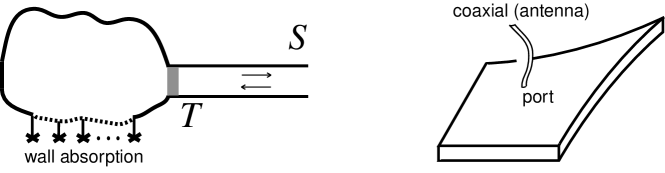
Figure 1: A sketch of a typical experimental setup with microwave billiards. A flat chaotic cavity is feeded with microwaves through an attached coaxial cable (i.e. a scattering channel). On average, $1-T$ part of the incoming flux, where $T\leq 1$ is the so-called transmission coefficient, is reflected back directly from the cable-cavity interface (port) without exciting long-lived resonances in the cavity. If the cavity is thin enough then only a transverse electric wave can propagate inside. The electric field has only a vertical component, which is uniform in vertical direction and distributed nontrivially in the plane. Therefore, there is a voltage between plates as well as a current due to the in-plane magnetic field. The impedance is a quantity which relates linearly the port voltage to the port current. Fluctuations of eigenmodes and eigenfrequencies result in fluctuations of the impedance or $S$-matrix, as the driving frequency or port position is changed.

Another insight to the same problem comes from looking at it not from the “outside”, but rather from the “inside”. Then the prime object of interest turns out to be the impedance $Z$ relating linearly voltages to currents at the system input [25, 26], see figure 1. By proper taking into account the wave nature of the current [27, 28] the cavity impedance can be seen as an electromagnetic analogue of Wigner’s reaction matrix of the scattering theory. This can be easily understood qualitatively through the well-known equivalence of the two-dimensional Maxwell equations to the Schrödinger equation, the role of the wave function being played by the electromagnetic field (the voltage in our case). Then the definition of the impedance becomes formally similar to the definition of the reaction matrix (which relates linearly the scattering wave function to its normal derivative on the boundary). The impedance is, therefore, related to the local Green’s function of the closed cavity and fluctuates strongly due to chaotic internal dynamics.

The imaginary part of the local Green’s function (which is proportional to the real part of $Z$) is well known as the local density of states (LDoS) and has a long story of studies in disordered electronic systems, see [29] for a recent review. Actually, a closely related quantity emerges in the context of spectra of complex atoms and molecules where it has the meaning of the total cross-section of indirect photoabsorption [30] (see also [31, 32]). It also appears in studies on spontaneous light emission by atoms placed in chaotic cavities [33]. As to the real part of the Green’s function, it seems to have no direct physical meaning in mesoscopics while it has the meaning of reactance in electromagnetics, where both real and imaginary parts are experimentally accessible.

In this review we discuss an approach developed recently by us in short communications [21, 22, 34] which treats both inside and outside aspects of the problem on equal footing. In this capacity it provides a uniform and deeper understanding of various results on absorptive scattering obtained earlier in [16, 17, 18]. In particular, the method allows one to study very efficiently the distribution of the local Green’s function (complex impedance) at arbitrary absorption and to relate it to that of reflection, thus linking somewhat complementary experiments [10] and [25] together. Although calculations are most explicit and simple for fully chaotic systems, when one can rely upon the random matrix theory (RMT), our method actually has relevance in a much broader context beyond RMT that involves many interesting aspects of disordered mesoscopic systems with absorption, including effects of the Anderson localisation. From that point of view, the method opens an attractive possibility to look at some long-standing problems (e.g. statistics of time delays) from a different perspective, see [35] as well as subsections 4.1.6 and 4.1.7 below.

2 Reflection, time delays and resonance spectrum

In this section, we provide a short description of the scattering approach to the problem. The resonance energy dependence of observables becomes explicit in the well-known Hamiltonian approach to quantum scattering, which was developed first in the context of nuclear physics [2, 36, 37, 38] and can be easily adopted for models emerging in quantum chaotic scattering and mesoscopic physics, see e.g. [4, 39, 40, 41] for reviews. This framework turns out to be also most suited to take a finite absorption into account. The starting point is the following fundamental relation between the resonance part of the scattering matrix and the Wigner’s reaction matrix $K$:

$$S(E)=\frac{1-\rmi K(E)}{1+\rmi K(E)}\,,\qquad K(E)={\textstyle\frac{1}{2}}V^{{\dagger}}(E-H)^{-1}V\,.$$ (1)

The Hermitian Hamiltonian $H$ of the closed system gives rise to $N$ real energy levels (eigenfrequencies). Those are coupled to $M$ continuum channels via the $N{\times}M$ matrix $V$ of coupling amplitudes $V^{c}_{n}$ ($n=1\ldots N$, $c=1\ldots M$), and as a result are converted to $N$ complex resonances. To see this, we expand (1) in a Taylor series in $K$ and, after regrouping the terms, bring the resulting expression to another well known form

$$S(E)=1-\rmi V^{{\dagger}}\frac{1}{E-\mathcal{H}_{\mathrm{eff}}}V\,,\qquad\mathcal{H}_{\mathrm{eff}}=H-{\textstyle\frac{\rmi}{2}}VV^{{\dagger}}\$$ (2)

for the $S$-matrix. The effective Hamiltonian $\mathcal{H}_{\mathrm{eff}}$ emerging here characterises the open system and is the non-Hermitian counterpart of $H$. The factorized structure of the anti-Hermitian part is necessary to ensure the unitarity of $S$. The coupling amplitudes $V$ change very slowly with the energy (far from the channels thresholds) and one can safely consider them to be energy-independent. In such a resonance approximation the complex eigenvalues $\mathcal{E}_{n}=E_{n}-{\textstyle\frac{\rmi}{2}}\Gamma_{n}$ of $\mathcal{H}_{\mathrm{eff}}$, with the energies $E_{n}$ and escape widths $\Gamma_{n}>0$, are the only singularities of the $S$ matrix in the complex energy plane. As required by causality [42], they are located in the lower half plane and correspond to the long-lived resonance states formed on the intermediate stage of a scattering process. The corresponding (left and right) eigenvectors form the so-called bi-orthogonal system. Recent discussion concerning applicability of the effective Hamiltonian approach to potential scattering problems (like those with cavities) can be found in [43, 44, 45, 46].

Flux conservation requires $S(E)$ to be unitary at the real values of $E$. It is useful to define at real $\Omega$ the following matrix

$$R_{\Omega}(E)\equiv S^{{\dagger}}(E-{\textstyle\frac{1}{2}}\Omega)S(E+{\textstyle\frac{1}{2}}\Omega)=1+\rmi\Omega V^{{\dagger}}\frac{1}{E-{\textstyle\frac{1}{2}}\Omega-\mathcal{H}_{\mathrm{eff}}^{{\dagger}}}\frac{1}{E+{\textstyle\frac{1}{2}}\Omega-\mathcal{H}_{\mathrm{eff}}}V\,.$$ (3)

The second equality here results from the substitution of (2) and then making use of the identity $\rmi VV^{{\dagger}}+\Omega=(E+{\textstyle\frac{1}{2}}\Omega-\mathcal{H}_{\mathrm{eff}})-(E-{\textstyle\frac{1}{2}}\Omega-\mathcal{H}_{\mathrm{eff}}^{{\dagger}})$ which leads to cancellations of the cross-terms. Expression (3) tends to unity as $\Omega\to 0$ and it is the Wigner-Smith time-delay matrix [47, 48] $Q(E)=-\rmi S^{{\dagger}}(E){\textstyle\frac{\rmd}{\rmd E}}S(E)=-\rmi{\textstyle\frac{\rmd}{\rmd\Omega}}R_{\Omega}(E)|_{\Omega=0}$ (we put $\hbar=1$) which determines the unitarity deficit of $R_{\Omega}$ to the linear order [49]:

$$R_{\Omega}(E)\simeq 1+\rmi\Omega Q(E)+O(\Omega^{2})\,,\qquad Q(E)=V^{{\dagger}}\frac{1}{(E-\mathcal{H}_{\mathrm{eff}})^{{\dagger}}}\frac{1}{E-\mathcal{H}_{\mathrm{eff}}}V\,.$$ (4)

Such a factorized representation [50] for the time-delay matrix (which contains no longer the energy derivative) is a consequence of the resonance approximation considered. It serves to make a connection of time delays to the resonance spectrum most explicit. The matrix element $Q^{cc^{\prime}}=(b^{{\dagger}}b)^{cc^{\prime}}$ may be physically interpreted as the scalar product (or “overlap”) between the internal parts $b^{c}=(E-\mathcal{H}_{\mathrm{eff}})^{-1}V^{c}$ of the scattering wave functions for waves incident in the channels $c$ and $c^{\prime}$, respectively [50]. In particular, the mean time delay in the channel $c$ given by the diagonal element $Q^{cc}$ coincides in such an approximation with the dwell time given by the norm of $b^{c}$. One should distinguish generally between $Q^{cc}$ and the so-called proper time-delays $q_{c}$ (eigenvalues of $Q$). Taking their sum, one comes to a weighted mean time delay characteristic $Q_{w}=\frac{1}{M}\tr Q=\frac{1}{M}\sum_{c}Q^{cc}=\frac{1}{M}\sum_{c}q_{c}$, the so-called Wigner’s time delay which is known, see e.g. [51, 49, 40], to be determined by the energy derivative of the total scattering phaseshift: $Q_{w}=-{\textstyle\frac{\rmi}{M}}\frac{\partial}{\partial E}\log\det{S}$. Diverse aspects of delay times in quantum chaotic scattering [40] as well as in a general quantum mechanical context [52, 53] can be found in the cited literature and references therein.

As is well known, statistics of spectra of closed quantum systems with chaotic classical counterparts are to a large extent universal and independent of their microscopic nature. This remarkable universality provides one with a possibility to use the RMT [54] for an adequate description of many physical properties of such systems [55]. According to the general paradigm we replace the actual Hermitian part $H$ of the effective Hamiltonian (2) with a random Hermitian matrix $H$ taken from one of the three canonical Wigner-Dyson’s ensembles labelled by the symmetry index $\beta$ according to the symmetry of the system under consideration. The Gaussian orthogonal (GOE, $\beta=1$ and $H$ real symmetric) and unitary (GUE, $\beta=2$ and $H$ Hermitian) ensembles stand for systems with preserved or fully broken time-reversal symmetry (TRS), respectively. The remaining Gaussian symplectic ensemble (GSE, $\beta=4$ and $H$ self-dual quaternion) is relevant for description of time-reversal systems with strong spin-orbit scattering. The limit of large $N\to\infty$ is supposed to be finally taken. Then eigenvalues are distributed on the finite interval according to Wigner’s semicircle law, which determines locally the mean level spacing $\Delta$. The most appealing feature of the RMT approach is that quantities related to spectral fluctuations when expressed in units of $\Delta$ (“unfolding”) do not depend on microscopic details (i.e. the particular form of the distribution of $H$ or the profile of $\Delta$) and become uniform throughout the whole spectrum [55]. For practical reasons we thus restrict ourselves to considering fluctuations at the center of the spectrum ($E=0$) only. Similarly, the results turn out to be also independent of particular statistical assumptions on coupling amplitudes $V^{c}_{n}$ as long as $M\ll N$ [56, 49]. The amplitudes may be chosen as fixed [2] or random [38] variables and enter final expressions only in combinations known as transmission coefficients (also sometimes called sticking probabilities)

$$T_{c}\equiv 1-|\overline{S^{cc}}|^{2}=\frac{4\kappa_{c}}{(1+\kappa_{c})^{2}}\,,\qquad\kappa_{c}=\frac{\pi\|V^{c}\|^{2}}{2N\Delta}$$ (5)

where $\overline{S^{cc}}$ stands for the average (optical) $S$ matrix. The transmission coefficients are assumed to be input parameters of the theory, the cases $T_{c}\ll 1$ and $T_{c}=1$ corresponding to an almost closed or perfectly open channel “c”, respectively.

Absorption is usually seen as a dissipation process, which evolves exponentially in time. Strictly speaking, different spectral components of the field may have different dissipation rates. However, frequently this rather weak energy dependence can easily be neglected as long as local fluctuations on much finer energy scale $\sim\Delta$ are considered. As a result, all the resonances acquire one and the same absorption width $\Gamma>0$ additionally to their escape widths $\Gamma_{n}$. The dimensionless phenomenological parameter $\gamma\equiv 2\pi\Gamma/\Delta$ characterizes then the absorption strength, with $\gamma\ll 1$ or $\gamma\gg 1$ corresponding to the weak or strong absorption limit, respectively. Microscopically, it can be modelled by means of a huge number of weakly open parasitic channels [6, 57] or by coupling to a very complicated background with almost continuous spectrum [16], see also [58]. In microwave billiards such an approximation is frequently very good to account for uniform Ohmic losses which happen everywhere in non-perfectly conducting walls. However, in some experimentally relevant situations as, e.g., complex reverberant structures [59] or even microwave cavities at room temperature [11, 46] an approximation of uniform absorption may break down, and one should take into account instead localized-in-space losses which will result in different broadenings of different modes. The latter are easily incorporated in the model by treating them as if induced by additional scattering channels, see e.g. [19]. An alternative scheme of treating localised-in-space surface absorption is discussed in [23]. (Discussion of a formal theory of scattering for complex absorbing potentials can be found in [60].)

Operationally, the uniform absorption can equivalently be taken into account by a purely imaginary shift of the scattering energy $E\to E+{\textstyle\frac{\rmi}{2}}\Gamma\equiv E_{\gamma}$, so that the $S$-matrix $S_{\gamma}(E)\equiv S(E_{\gamma})$ becomes subunitary. The reflection matrix $R_{\gamma}=S_{\gamma}^{{\dagger}}S_{\gamma}$ provides then a natural measure of the mismatch between incoming and outgoing fluxes. It can be obtained from $R_{\Omega}$, (3), by analytic continuation in $\Omega$ from a real to the purely imaginary value $\Omega=\rmi\Gamma$, yielding [16]:

$$R_{\gamma}(E)=R_{\Omega=\rmi\Gamma}(E)=1-\Gamma Q_{\gamma}(E)\,,\qquad Q_{\gamma}(E)\equiv V^{{\dagger}}\frac{1}{(E_{\gamma}-\mathcal{H}_{\mathrm{eff}})^{{\dagger}}}\frac{1}{E_{\gamma}-\mathcal{H}_{\mathrm{eff}}}V\,.$$ (6)

This representation is valid at arbitrary value of $\Gamma$. In the limit of small $\Gamma$ one can neglect the difference between $Q_{\gamma}$ and $Q$, resulting in the approximate expression [61, 15] $R_{\gamma}\simeq 1-\Gamma Q$ following from (4). It is therefore tempting to keep for $Q_{\gamma}$ the meaning of the time-delay matrix at finite absorption as well (see, however, discussion in [16]). By construction, $R_{\gamma}$ is a Hermitian matrix, its positive reflection eigenvalues $r_{c}=1-\Gamma q_{c}\leq 1$ are related to proper time-delays $q_{c}$ (at finite absorption).

Considering quantum scattering with no internal dissipation, $\Gamma=0$, the $S$-matrix unitarity ensures that the reflection coefficient $R_{c}=|S^{cc}|^{2}$ in any given channel is simply related to the quantum mechanical probability to exit via any of the remaining channels, known as the transmission probability: $R_{c}=1-\sum_{b\neq c}|S^{bc}|^{2}$. For an absorptive system the last equality is violated, but still the quantity $\tau_{c}=1-R_{c}$ can be interpreted as the quantum mechanical probability that a particle entering via a given channel never exits through the same channel. Hence it was suggested to call $\tau_{c}$ the probability of no return (PNR) [17]. In the particular case of a single open channel fluctuations of the PNR $\tau$ arise solely due to absorption (neglecting dissipation trivially results in $\tau\equiv 0$). At weak absorption $\tau\approx\Gamma q$ , so that the PNR is just simply proportional to the time-delay.

At last but not least, the matrix $Z\equiv\rmi K(E_{\gamma})$ has the meaning of the normalized cavity impedance in such a setting, see [27, 28] for further details.

3 Correlation functions

Any observable in chaotic resonance scattering exhibits strong fluctuations over a smooth background as the scattering energy or other external parameters are varied. Usually these variations occur on two essentially different energy scales. This fact is conventionally taken into account by decomposing fluctuating quantities into a mean part and a fluctuating part, the former being understood as the result of spectral or (assumed to be equivalent) ensemble average $\langle\cdots\rangle$. In this section we consider statistics as determined by a two-point correlation function of the fluctuating parts (frequently called a “connected” correlation function): $\left\langle AB\right\rangle_{\mathrm{conn}}=\left\langle AB\right\rangle-\left\langle A\right\rangle\left\langle B\right\rangle$. We restrict ourselves below to the cases of preserved ($\beta=1$) and broken ($\beta=2$) TRS (the symplectic case $\beta=4$ proceeds along the same lines).

3.1 Impedance

Let us start with considering the simplest case of the impedance correlations. The problem can be fully reduced to that of spectral correlations determined by the two-point cluster function $Y_{2,\beta}(\omega)=\delta(\omega)-\Delta^{2}\left\langle\rho(E_{1})\rho(E_{2})\right\rangle_{\mathrm{conn}}$, where $\omega=(E_{2}-E_{1})/\Delta$ and $\rho(E)$ being the level density. It is easy to satisfy oneself that for the mean impedance at $E=0$ holds $\left\langle Z^{ab}\right\rangle=\kappa_{a}\delta^{ab}$. To calculate the energy correlation function $C^{abcd}_{Z}(\omega)\equiv\left\langle Z^{ab*}(E_{1})Z^{cd}(E_{2})\right\rangle_{\mathrm{conn}}$, it is instructive to write $Z^{ab}(E)$ in the eigenbasis of the closed system: $Z^{ab}(E)={\textstyle\frac{\rmi}{2}}\sum_{n}v^{a*}_{n}v^{b}_{n}/(E-E_{n}+{\textstyle\frac{\rmi}{2}}\Gamma)$. A rotation that diagonalizes the (random) Hamiltonian matrix $H$ transforms the (fixed) coupling amplitudes $V^{a}_{n}$ to Gaussian distributed random coupling amplitudes $v^{a}_{n}$ with zero mean and covariances $\left\langle v^{a*}_{n}v^{b}_{m}\right\rangle=(2\kappa_{a}\Delta/\pi)\delta^{ab}\delta_{nm}$. In such a representation the energy correlation function acquires the following form:

$$C^{abcd}_{Z}(\omega)=\sum_{n,m}\frac{1}{4}\left\langle v^{a}_{n}v^{b*}_{n}v^{c*}_{m}v^{d}_{m}\right\rangle\left\langle\frac{1}{E_{1}-E_{n}-{\textstyle\frac{\rmi}{2}}\Gamma}\frac{1}{E_{2}-E_{m}+{\textstyle\frac{\rmi}{2}}\Gamma}\right\rangle_{\mathrm{conn}}$$ (7)

and the averaging over coupling amplitudes and that over the spectrum can be done independently. The Gaussian statistics of $v$ results in

$${\textstyle\frac{1}{4}}({\textstyle\frac{\pi}{\Delta}})^{2}\left\langle v^{a}_{n}v^{b*}_{n}v^{c*}_{m}v^{d}_{m}\right\rangle=\kappa_{a}\kappa_{c}\delta^{ab}\delta^{cd}+\kappa_{a}\kappa_{b}(\delta^{ac}\delta^{bd}+\delta_{1\beta}\delta^{ad}\delta^{bc})\delta_{nm}$$ (8)

where $\delta_{1\beta}$ term accounts for the presence of TRS, when all $v^{a}_{n}$ are real and $Z$ is symmetric. It is useful to represent the spectral correlation function in a form of the Fourier integral $\int_{0}^{\infty}\rmd t_{1}\int_{0}^{\infty}\rmd t_{2}e^{-\Gamma(t_{1}+t_{2})/2}e^{\rmi E(t_{2}-t_{1})}e^{\rmi(E_{2}-E_{1})(t_{1}+t_{2})/2}\left\langle e^{\rmi(E_{n}t_{1}-E_{m}t_{2})}\right\rangle_{\mathrm{conn}}$. Due to the uniformity of local fluctuations in the bulk of the spectrum, one can integrate additionally over the position $E$ of the mean energy: $\int\!\frac{\rmd E}{N\Delta}e^{\rmi E(t_{2}-t_{1})}={\textstyle\frac{1}{N}}\delta(\frac{t_{2}-t_{1}}{t_{H}})$, where $t_{H}\equiv 2\pi/\Delta$ is the Heisenberg time. It is natural therefore to measure the time in units of $t_{H}$. From the known RMT spectral fluctuations one also has for $n{\neq}m$ $(1-N)\left\langle e^{2\pi\rmi(E_{n}-E_{m})t/\Delta}\right\rangle_{\mathrm{conn}}=b_{2,\beta}(t)$, where $b_{2,\beta}(t)$ is the spectral form factor defined through the Fourier transform of $Y_{2,\beta}(\omega)=\int_{-\infty}^{\infty}\!\rmd te^{2\pi\rmi\omega t}b_{2,\beta}(t)$ [54, 55]:

$$b_{2,\beta=1}(t)=[1-2t+t\log(1+2t)]\Theta(1-t)+[t\log({\textstyle\frac{2t+1}{2t-1}})-1]\Theta(t-1)$$ (9a)

$$b_{2,\beta=2}(t)=(1-t)\Theta(1-t)$$ (9b)

at $t>0$ and $b_{2,\beta}(-t)=b_{2,\beta}(t)$. Combining all these together, we arrive finally at

$$C^{abcd}_{Z}(\omega)=\int_{0}^{\infty}\!\!\!\rmd te^{2\pi\rmi\omega t}\hat{C}^{abcd}_{Z}(t)$$ (9ja)

$$\hat{C}^{abcd}_{Z}(t)=4\,e^{-\gamma t}\,[\kappa_{a}\kappa_{c}[1-b_{2,\beta}(t)]\delta^{ab}\delta^{cd}+\kappa_{a}\kappa_{b}(\delta^{ac}\delta^{bd}+\delta_{1\beta}\delta^{ad}\delta^{bc})]\,.$$ (9jb)

Similar in spirit calculations were done in a context of reverberation in complex structures in [62, 59] and in a context of chaotic photodissociation in [63, 64].

The form factor (9jb) is simply related to that of $K$ matrix elements at zero absorption as $\hat{C}^{abcd}_{Z}(t)=e^{-\gamma t}\hat{C}^{abcd}_{K}(t)$. Such a relationship between the corresponding form factors with and without absorption is generally valid for any correlation function which may be reduced to the two-point correlation function of resolvents (see [7] and the discussion below, e.g., for the case of the $S$ matrix). This can be easily understood as a result of the analytic continuation $2\pi\omega\to 2\pi\omega+i\gamma$ of the energy difference $\omega$ reflecting switching on the absorption (see the previous section).

The obtained expressions describe a gradual loss of correlations in $Z$ matrix elements as the energy difference grows; generally, $C_{Z}(\omega{\to}\infty)\to 0$. At $\omega=0$, (9ja) provides us with impedance variances $C_{Z}^{abab}(0)=\mathrm{var}(Z^{ab})\equiv\langle|Z^{ab}|^{2}\rangle-|\langle{Z^{ab}}\rangle|^{2}$, which were recently studied experimentally in [65]. In analogy with the so-called elastic enhancement factor considered frequently in nuclear physics [66], one can define the following ratio of variances in reflection ($a{=}b$) to that in transmission ($a{\neq}b$):

$$W_{Z,\beta}\equiv\frac{\sqrt{\mathrm{var}(Z^{aa})\mathrm{var}(Z^{bb})}}{\mathrm{var}(Z^{ab})}=2+\delta_{1\beta}-\int_{0}^{\infty}\!\!\rmd s\,e^{-s}b_{2,\beta}({\textstyle\frac{s}{\gamma}})$$ (9jk)

where the second equality follows easily from (9jb) (note that the coupling constants $\kappa_{a,b}$ are mutually cancelled here). Making use of $b_{2,\beta}(\infty){=}0$ and $b_{2,\beta}(0){=}1$, one can readily find $W_{Z,\beta}$ in the limiting cases of weak or strong absorption as:

$$W_{Z,\beta}=\cases{2+\delta_{1\beta}&at $\gamma\ll 1$\\ 1+\delta_{1\beta}&at $\gamma\gg 1$\\ }\,.$$ (9jl)

$W_{Z,\beta}$ decays monotonically as absorption grows. In the case of unitary symmetry, (9b) and (9jk) yield explicitly $W_{Z,2}=1+{\textstyle\frac{1}{\gamma}}(1-e^{-\gamma})$ in agreement with [65]. It is hardly possible to get a simple explicit expression at finite $\gamma$ in the case of orthogonal symmetry. However, a reasonable approximation can be found if one notices that the integration in (9jk) is determined mainly by the region $s\leq 1$, so that one can approximate $b_{2,1}(s)\approx(1-2s+2s^{2})\Theta(1-s)$ through its Taylor expansion. Performing the integration, one arrives at $W_{Z,1}\approx 3-\gamma^{-2}[(4+\gamma^{2})(1-e^{-\gamma})-2\gamma(1+e^{-\gamma})]$, which turns out to be a good approximation to the exact answer at moderately strong absorption (deviations are seen numerically only at $\gamma\sim 1$).

3.2 Scattering matrix

The energy correlation function of the scattering matrix elements

$$C^{abcd}_{S}(\omega)\equiv\left\langle S_{\gamma}^{ab*}(E_{1})S_{\gamma}^{cd}(E_{2})\right\rangle_{\mathrm{conn}}=\int_{0}^{\infty}\!\!\rmd te^{2\pi\rmi\omega t}\hat{C}^{abcd}_{S}(t)$$ (9jm)

is a much more complicated object for an analytical consideration as compared to (7). The reason becomes clear if one considers again the pole representation of the $S$ matrix which follows from (2): $S^{ab}(E)=\delta^{ab}-\rmi\sum{w^{a}_{n}\tilde{w}^{b}_{n}}/(E-\mathcal{E}_{n})$. Due to unitarity constraints imposed on $S$ at real $E$ the residues and complex resonance energies develop nontrivial correlations [38]. Although results on statistics of resonances in the complex plane [40, 67, 68, 69] as well as the corresponding residues [69, 70] became recently available in some particular cases, this knowledge is insufficient as yet for calculating $S$-matrix correlations in general. The separation like (7) into a “coupling” and “spectral” average is no longer possible and can be done only by involving some approximations [71]. The powerful supersymmetry method [72, 2] turns out to be an appropriate technique to perform the statistical average in this case. In their seminal paper [2], Verbaarschot, Weidenmüller and Zirnbauer performed the exact calculation of (9jm) at arbitrary transmission coefficients (and zero absorption) in the case of orthogonal symmetry. This finding was later adopted [7] to include absorption. The corresponding exact result for unitary symmetry has been recently presented by us in [34] (see also [73] concerning the $S$-matrix variance in the GOE-GUE crossover at perfect coupling) and is discussed below.

The calculation proceeds along the same lines as in [2]. The final expression for both the connected correlation function and its form factor (9jm) can be equally represented as follows:

$$C^{abcd}_{S}=\delta^{ab}\delta^{cd}T_{a}T_{c}\sqrt{(1-T_{a})(1-T_{c})}J_{ac}+(\delta^{ac}\delta^{bd}+\delta_{1\beta}\delta^{ad}\delta^{bc})T_{a}T_{b}P_{ab}\,.$$ (9jn)

Here, the $\delta_{1\beta}$ term accounts trivially for the symmetry property $S^{ab}=S^{ba}$ in the presence of TRS. $J_{ac}$ and $P_{ab}$ defined below are some functions (of the energy difference $\omega$ or the time $t$), which depend also on TRS, coupling and absorption but already in a nontrivial way. As a result, the elastic enhancement factor $W_{S,\beta}\equiv\sqrt{\mathrm{var}(S^{aa})\mathrm{var}(S^{bb})}/\mathrm{var}(S^{ab})$ is generally a complicated function of all these parameters, in contrast to (9jk). In the particular case of perfect coupling, all $T_{c}=1$, one has obviously from (9jn) that $W_{S,\beta}=1+\delta_{1\beta}$ at any absorption strength.

We consider first expression (9jn) in the energy domain at real $\omega$ (no absorption). The functions $J_{ac}(\omega)$ and $P_{ab}(\omega)$ can be generally written as certain expectation values in the field theory (nonlinear zero-dimensional supersymmetric $\sigma$-model) whose explicit representations depend on the symmetry case considered, we refer the reader to [2, 74] for general discussion. In the $\beta=1$ case of orthogonal symmetry the well-known result of [2] reads as follows:

$$J_{ac}(\omega)=\textstyle\left\langle\bigl{(}\frac{\mu_{1}}{1+T_{a}\mu_{1}}+\frac{\mu_{2}}{1+T_{a}\mu_{2}}+\frac{\mu_{0}}{1-T_{a}\mu_{0}}\bigr{)}\bigl{(}\frac{\mu_{1}}{1+T_{c}\mu_{1}}+\frac{\mu_{2}}{1+T_{c}\mu_{2}}+\frac{\mu_{0}}{1-T_{c}\mu_{0}}\bigr{)}\mathcal{F}_{M}\right\rangle_{\mu}$$ (9joa)

$$\textstyle P_{ab}(\omega)=\textstyle\left\langle\bigl{(}\frac{\mu_{1}(1+\mu_{1})}{(1+T_{a}\mu_{1})(1+T_{b}\mu_{1})}+\frac{\mu_{2}(1+\mu_{2})}{(1+T_{a}\mu_{2})(1+T_{b}\mu_{2})}+\frac{\mu_{0}(1-\mu_{0})}{(1-T_{a}\mu_{0})(1-T_{b}\mu_{0})}\bigr{)}\mathcal{F}_{M}\right\rangle_{\mu}$$ (9job)

with $\mathcal{F}_{M}=\prod_{c}[\frac{(1-T_{c}\mu_{0})^{2}}{(1+T_{c}\mu_{1})(1+T_{c}\mu_{2})}]^{1/2}$ being the so-called “channel factor”, which accounts for system openness, and $\langle(\cdots)\rangle_{\mu}$ is to be understood explicitly as

$$\frac{1}{8}\int_{0}^{\infty}\!\rmd\mu_{1}\!\int_{0}^{\infty}\!\rmd\mu_{2}\!\int_{0}^{1}\!\rmd\mu_{0}\frac{(1-\mu_{0})\mu_{0}|\mu_{1}-\mu_{2}|\,e^{\rmi\pi\omega(\mu_{1}+\mu_{2}+2\mu_{0})}}{[(1+\mu_{1})\mu_{1}(1+\mu_{2})\mu_{2}]^{1/2}(\mu_{0}+\mu_{1})^{2}(\mu_{0}+\mu_{2})^{2}}\left(\ldots\right)\,.$$ (9jop)

In the $\beta=2$ case of unitary symmetry we have found [34] that

$$J_{ac}(\omega)=\textstyle\left\langle\bigl{(}\frac{\mu_{1}}{1+T_{a}\mu_{1}}+\frac{\mu_{0}}{1-T_{a}\mu_{0}}\bigr{)}\bigl{(}\frac{\mu_{1}}{1+T_{c}\mu_{1}}+\frac{\mu_{0}}{1-T_{c}\mu_{0}}\bigr{)}\mathcal{F}_{M}\right\rangle_{\mu}$$ (9joqa)

$$\textstyle P_{ab}(\omega)=\textstyle\left\langle\bigl{(}\frac{\mu_{1}(1+\mu_{1})}{(1+T_{a}\mu_{1})(1+T_{b}\mu_{1})}+\frac{\mu_{0}(1-\mu_{0})}{(1-T_{a}\mu_{0})(1-T_{b}\mu_{0})}\bigr{)}\mathcal{F}_{M}\right\rangle_{\mu}$$ (9joqb)

with the channel-factor $\mathcal{F}_{M}=\prod_{c}\frac{1-T_{c}\mu_{0}}{1+T_{c}\mu_{1}}$ and the corresponding integration being

$$\int_{0}^{\infty}\!\rmd\mu_{1}\int_{0}^{1}\!\rmd\mu_{0}(\mu_{1}+\mu_{0})^{-2}\,e^{\rmi 2\pi\omega(\mu_{1}+\mu_{0})}\left(\ldots\right)\,.$$ (9joqr)

In the important particular case of the single open channel (elastic scattering), the general expression for the $\beta=2$ case simplifies further to

$$\left\langle S^{*}(E_{1})S(E_{2})\right\rangle_{\mathrm{conn}}=T^{2}\int_{0}^{\infty}\!\rmd\mu_{1}\int_{0}^{1}\!\frac{\rmd\mu_{0}}{\mu_{1}+\mu_{0}}\frac{1+(2-T)\mu_{1}}{(1+T\mu_{1})^{3}}\,e^{\rmi 2\pi\omega(\mu_{1}+\mu_{0})}\,.$$ (9joqs)

Finally, putting above $\omega\to\omega+\rmi\gamma/2\pi$ accounts for the finite absorption strength $\gamma$.

To consider (9jn) in the time domain, i.e. the form factor $\hat{C}^{abcd}_{S}(t)$, we notice that the variable $t={\textstyle\frac{1}{2}}(\mu_{1}+\mu_{2}+2\mu_{0})$ for $\beta=1$ or $t=\mu_{1}+\mu_{0}$ for $\beta=2$ plays the role of the dimensionless time (in units of $t_{H}$). The corresponding expressions for $\hat{P}_{ab}(t)$ and $\hat{J}_{ac}(t)$ can be investigated using the methods developed in [66, 71, 41]. For orthogonal symmetry it was done in [7], where the overall decaying factor $e^{-\gamma t}$ due to absorption was also confirmed by comparison to the experimental result for the form factor measured in microwave cavities. It is useful for the qualitative description to note that $\hat{P}_{ab}(t)$ and $2\hat{J}_{ac}(t)$ are quite similar to the “norm leakage” decay function [75] and the form factor of the Wigner’s time delays [49], respectively (they would coincide exactly at $\gamma=0$, if we put $T_{a,b,c}=0$ appearing explicitly in denominators above). Then one can follow analysis performed there, see also [41], to find $\hat{P}_{ab}(t)\approx e^{-\gamma t}$ and $\hat{J}_{ac}(t)\approx(2t/\beta)e^{-\gamma t}$ as exact asymptotic at small times [71], while they both become proportional to $e^{-\gamma t}t^{-M\beta/2-2}$ at large times.

Such a power law is characteristic for open systems [39, 41, 75]. Physically, it results from width fluctuations, which diminish as the number $M$ of open channels grows [40, 75]. In the limiting case $M\to\infty$ and $T_{c}\to 0$, all the resonances acquire just the same escape width $\sum_{c}T_{c}$ (in units of $t_{H}^{-1}$), which is often called the Weisskopf’s width [76], so that the total width is $\gamma_{T}=\sum_{c}T_{c}+\gamma$. Then there occur further simplifications: $\hat{P}_{ab}(t)=e^{-\gamma_{T}t}$ and $\hat{J}_{ab}(t)=[1-b_{2,\beta}(t)]e^{-\gamma_{T}t}$, that results finally in

$$C^{abcd}_{S}(\omega)=\frac{(\delta^{ac}\delta^{bd}+\delta_{1\beta}\delta^{ad}\delta^{bc})T_{a}T_{b}}{\gamma_{T}-2\pi\rmi\omega}+\delta^{ab}\delta^{cd}T_{a}T_{c}\int_{0}^{\infty}\!\rmd t[1-b_{2,\beta}(t)]e^{-(\gamma_{T}-2\pi\rmi\omega)t}.$$ (9joqt)

For the case of $\beta=1$ this result (at zero absorption) was obtained earlier by Verbaarschot [66]. In the limit considered, expression (9joqt) is very similar to (9ja), (9jb), so that the enhancement factor $W_{S,\beta}$ is given by the same (9jk) where $\gamma$ is to be substituted with $\gamma_{T}$. At $\gamma_{T}\gg 1$ (large resonance overlapping or strong absorption, or both) the dominating term in (9joqt) is the first one, which is known as the Hauser-Feshbash relation [77], see [78, 79, 80] for discussion. Then $W_{S,\beta}=2/\beta=W_{Z,\beta}$ that can be also understood as the consequence of the gaussian statistics of $S$ (as well as of $Z$) in the limit of strong absorption [80].

3.3 Reflection

In this subsection we consider fluctuations in the weighted-mean reflection coefficient defined as $r={\textstyle\frac{1}{M}}\tr R$. Its average value $\left\langle r\right\rangle$ was recently calculated in [16], where the following exact result was found to be

$$\langle{r}\rangle=1-\frac{\gamma}{M}\left[1-\gamma\int_{0}^{\infty}\!\!\rmd t\,e^{-\gamma t}P(t)\right]$$ (9joqu)

relating $\left\langle r\right\rangle$ to the so-called “norm-leakage” function $P(t)$ introduced in [75]. The actual value of $\left\langle r\right\rangle$ changes with growing absorption between $1-\frac{\gamma}{M}$ at $\gamma\ll 1$ and $1-\frac{1}{M}\sum_{c}T_{c}$ at $\gamma\gg M$. For the sake of simplicity we consider the case of $M$ equivalent channels below, all $T_{c}=T$. For large $M\gg 1$ the widths cease to fluctuate, yielding $P(t)=e^{-MTt}$, so that (9joqu) results in $\left\langle r\right\rangle=(MT+\gamma(1-T))/(MT+\gamma)$ [18].

The correlation function $C_{R}(\omega)=\left\langle r(E_{1})r(E_{2}\right\rangle_{\mathrm{conn}}=\Gamma^{2}\left\langle Q_{w}(E_{1})Q_{w}(E_{2}\right\rangle_{\mathrm{conn}}$ is simply related by virtue of (6) to that of Wigner’s time delay $Q_{w}={\textstyle\frac{1}{M}}\tr{Q_{\gamma}}$ (at finite $\Gamma$). Amounting to a four-point correlation function of resolvents, its evaluation is generally beyond the present day state of art in the supersymmetry method. However, by approximating $Q_{w}\approx\frac{1}{M}\sum_{n}\Gamma_{n}/[(E-E_{n})^{2}+{\textstyle\frac{1}{4}}(\Gamma_{n}+\Gamma)^{2}]$, cf. (6), and making use of the rescaled Breit-Wigner approximation (RBWA) of Gorin and Seligman [71], one can find an expression which is supposed [7] to work reasonably well at finite absorption. The final result can be naturally represented in the form of the Fourier-integral

$$C_{R}(\omega)=\frac{2\gamma^{2}}{M^{2}}\int_{0}^{\infty}\!\rmd t\cos(2\pi\omega t)\,e^{-\gamma t}F_{R}(t)$$ (9joqv)

where the form-factor (we have set apart in (9joqv) the trivial absorbing factor $e^{-\gamma t}$) is

$$F_{R}(t)=\frac{c_{2,\beta}(t)}{(1+2Tt/\beta)^{M\beta/2}}-\frac{b_{2,\beta}(t)\,c_{1,\beta}({\textstyle\frac{t}{2}})^{2}}{(1+Tt/\beta)^{M\beta}}$$ (9joqw)

with the function $c_{n,\beta}(t)$, $n=1,2$, defined as follows:

$$c_{n,\beta}(t)=\prod_{l=0}^{n-1}({\textstyle\frac{1}{2}}M\beta+l)\int_{0}^{\infty}\!\rmd x\frac{x^{n-1}\,e^{-(\beta\gamma/2T)(1+2Tt/\beta)x}}{(1+x)^{M\beta/2+n}}\,.$$ (9joqx)

It is instructive to consider the limiting cases of weak and strong absorption in more detail. At $\gamma\ll T\leq 1$, the $\gamma$-dependence and thus $t$-dependence of $c_{n,\beta}(t)$ is very weak, so that $c_{n,\beta}(t)\approx 1$ for $t\ll 1/\gamma$. As a result, the form-factor reduces to

$$F_{R}(t)=(1+2Tt/\beta)^{-M\beta/2}-b_{2,\beta}(t)(1+Tt/\beta)^{-M\beta}$$ (9joqy)

which is, as expected, just the form-factor of the Wigner’s time-delay correlation function at zero absorption calculated in the same scheme RBWA. In the opposite limiting case $\gamma\gg T$, the $x$-integration in $c_{n,\beta}(t)$ is determined mainly by the region of small $x\leq{T/\gamma}\ll 1$, that yields readily

$$F_{R}(t)=\left(\frac{MT}{\gamma}\right)^{2}\left[\frac{1+2/M\beta}{(1+2Tt/\beta)^{M\beta/2+2}}-\frac{b_{2,\beta}(t)}{(1+Tt/\beta)^{M\beta+2}}\right]\,.$$ (9joqz)

Comparing the large time asymptotic of $F_{R}(t)$, one sees that a crossover from $t^{-M\beta/2}$ to $t^{-M\beta/2-2}$ behavior happens at $\gamma\sim T$, as we go from weak to strong absorption regime. This behaviour is indicative of an additional decay of correlations induced by strong absorption on top of the pure exponential one. It is most pronounced for a single-channel cavity with TRS, corresponding to changing from $t^{-1/2}$ to $t^{-5/2}$.

4 Distribution functions

4.1 Single-channel scattering

4.1.1 Reflection coefficient and the local Green function.

It is quite clear, that the joint distribution of the real and imaginary parts of $K$

$$\mathcal{P}(u,v)=\left\langle\delta(u-\mathrm{Re\,}K)\,\delta(v+\mathrm{Im\,}K)\right\rangle$$ (9joqaa)

determines fully the statistics of the impedance and the $S$-matrix. By definition (1), $K=\kappa(N\Delta/\pi)G_{ii}$ is related to the diagonal element $G_{ii}=\langle{i}|(E_{\gamma}-H)^{-1}|i\rangle$ of the Green function of the closed system in the position representation, taken at the position $i$ of channel attachment. The RMT assumption for $H$ implies however that the basis of representation may be chosen arbitrary. One studies, therefore, statistics of the dimensionless local Green function $K\equiv u-iv$, with $v>0$ being the local density of states (LDoS). We consider first the case of perfect coupling $\kappa=1$ ($T=1$). In particular, this choice ensures the normalisation of the mean LDoS such that $\langle{v}\rangle=1$.

In this case, the following general form of the distribution function

$${\mathcal{P}}(u,v)=\frac{1}{2\pi v^{2}}P_{0}(x)\,,\qquad x=\frac{u^{2}+v^{2}+1}{2v}>1.$$ (9joqab)

may be easily established [21]. It initially emerged in [81, 82] in the course of tedious calculations for the $\beta{=}2$ symmetry class, but neither origin nor generality of such a form were appreciated. Actually, the validity of the form (9joqab) follows directly from exploiting the two following fundamental properties of the $S$-matrix statistics at perfect coupling: (i) the uniform distribution of the scattering phase $\theta\in(0,2\pi)$; and (ii) the statistical independence of $\theta$ and the $S$ matrix modulus. In the cases of chaotic systems with pure symmetries, both these properties can be verified making use of methods of [57]. In this paper we are proving (9joqab) directly by an alternative, more powerful method [22]. It holds much beyond the universal RMT regime for a very broad class of disordered Hamiltonians, in particular for the case when localisation effects already play an important role. Moreover, this method will help us to verify that (9joqab) holds in the crossover regime between the pure ensembles. For the time being the uniformity of the scattering phase distribution will be taken for granted.

Substituting $K=u-\rmi v$ into (1), we can immediately infer that the variable $x$ is directly related to the reflection coefficient, parameterizing it in the following way:

$$S_{\gamma}\equiv\sqrt{r}e^{\rmi\theta}\,,\qquad r=\frac{x-1}{x+1}\,,\qquad\cot\theta=\frac{u^{2}+v^{2}-1}{2u}\,.$$ (9joqac)

The joint distribution $\mathcal{P}(u,v)$ of $u$ and $v$ and that $P(x,\theta)$ of $x$ and $\theta$ are related by means of the Jacobian $|\frac{\partial(u,v)}{\partial(x,\theta)}|=v^{-2}$ as can be verified by a straightforward calculation. Finally, $P(x,\theta)=\frac{1}{2\pi}P_{0}(x)$ results from the uniform distribution of the phase and in this way $P_{0}(x)$ acquires the physical meaning of the normalized distribution of the reflection parameter $x$.

Relationship (9joqab) is one of our central results, which despite its apparent simplicity will have many far-reaching consequences which are not easy to guess otherwise. Let us note the invariance property of this distribution under the change $iK\to 1/iK$, meaning that both the impedance and its inverse (i.e. the admittance) must have one and the same probability distribution. Another remarkable feature of (9joqab) is, that it relates the distribution of the local Green function in the completely closed system to the distribution of the reflection coefficient in the perfectly open one. This fact will be fully utilised later on for extracting statistical properties of the Wigner time delay.

It is instructive to discuss first the exact limiting statistics

$$P_{0}(x)=\left\{\begin{array}[]{ll}\frac{\alpha^{\beta/2+1}}{2\Gamma(\beta/2+1)}\left(\frac{x+1}{2}\right)^{\beta/2}e^{-\alpha(x+1)/2}&(\alpha\ll 1)\\[8.61108pt] {\textstyle\frac{\alpha}{2}}\,e^{-\alpha(x-1)/2}&(\alpha\gg 1)\end{array}\right.\,,\qquad\alpha\equiv{\textstyle\frac{1}{2}}\beta\gamma\,,$$ (9joqad)

which can be found [21] in the weak or strong absorption limit. In the former case, one can follow [61, 15] in using a perturbation theory to relate reflection to the time delay in the ideal cavity without absorption (see (6) thereafter). The latter quantity has a known distribution [40, 83] $\mathcal{P}_{\tau}(\tau={\textstyle\frac{q}{t_{H}}})=[({\textstyle\frac{\beta}{2}})^{\beta/2}/\Gamma({\textstyle\frac{\beta}{2}})]\tau^{-\beta/2-2}e^{-\beta/2\tau}$ , which yields the first line above. In the opposite case of strong absorption, the real and imaginary parts of $S$-matrix become statistically independent Gaussian distributed variables [80, 14], resulting in the so-called Rayleigh distribution $P(r)\simeq(\gamma\beta/2)e^{-r\gamma\beta/2}$ of reflection valid at $r\approx{\textstyle\frac{1}{2}}(x-1)\ll 1$, and the second line in (9joqad) follows.

As to arbitrary absorption, an exact result was obtained first for unitary symmetry ($\beta=2$) by Beenakker and Brouwer [15]. It is convenient to keep the scaled absorption parameter $\alpha$, representing their result in the following form

$$P_{0}(x)=\frac{{\mathcal{N}}_{\beta}}{2}\left[A\,\left(\alpha(x+1)/2\right)^{\beta/2}+B\right]e^{-\alpha(x+1)/2}$$ (9joqae)

with $\alpha$-dependent constants $A\equiv e^{\alpha}-1$ and $B\equiv 1+\alpha-e^{\alpha}$, and with $\mathcal{N}_{2}=1$ standing for the normalization. For the case of symplectic symmetry ($\beta=4$), the exact form was reported very recently [21]. The explicit derivation is given in Appendix A, the final result being:

$$P_{0}^{\mathrm{gse}}(x)=\widetilde{P}_{0}^{\mathrm{gue}}(x)+\Bigl{[}\frac{\gamma^{2}}{2}(x+1)^{2}-\gamma(\gamma+1)(x+1)+\gamma\Bigr{]}\,e^{-\gamma x}\!\int_{0}^{\gamma}\!\!\rmd t\frac{\sinh{t}}{t}$$ (9joqaf)

where $\widetilde{P}_{0}^{\mathrm{gue}}(x)$ is the distribution (9joqae) for $\beta=2$ taken, however, at $\alpha=2\gamma$. The case of orthogonal symmetry, the most welcomed experimentally, turns out to be extremely tricky. It was suggested in [21], see also [10], that expression (9joqae) (with $\mathcal{N}_{\beta}=\alpha/(A\Gamma(\beta/2{+}1,\alpha)+Be^{-\alpha})$ and $\Gamma(\nu,\alpha)=\int_{\alpha}^{\infty}\!\rmd p\,p^{\nu-1}e^{-p}$) is an appropriate interpolation formula at $\beta=1$. It incorporates correctly both known limiting cases of weak or strong absorption and a reasonable agreement with available numerical and experimental data was found there in a broad range of the absorption strength. Below we provide an exact analytical treatment of this case by the method suggested in [22].

4.1.2 $\mathcal{P}(u,v)$ and the spectral correlation function of Green’s function resolvents.

We establish now the general relation [22] between the joint distribution function (9joqab) at arbitrary finite absorption and the energy autocorrelation function

$$C_{\Omega}(z_{-},z_{+})=\left\langle\frac{1}{z_{-}-\rmi 0-K_{0}(E-{\textstyle\frac{1}{2}}\Omega-\rmi 0)}\frac{1}{z_{+}+\rmi 0-K_{0}(E+{\textstyle\frac{1}{2}}\Omega+\rmi 0)}\right\rangle$$ (9joqag)

of the resolvents of the local Green function $K_{0}$ at zero absorption ($\Gamma=0$, indicated explicitly in this subsection with the subscript “0”). Distribution (9joqab) can be obtained from (9joqag) by analytic continuation in $\Omega$ from a real to purely imaginary value $\Omega=\rmi\Gamma$ as follows. $K_{0}(E)$ is an analytic function of the energy in the upper or lower half-plane and, thus, can be analytically continued to the complex values: $K_{0}(E\pm{\textstyle\frac{\rmi}{2}}\Gamma)\equiv u\mp\rmi v$, $v>0$. This allows us to continue then analytically the correlation function (9joqag) from a pair of its real arguments to the complex conjugate one: $z_{+}=(z_{-})^{*}\equiv z^{\prime}+\rmi z^{\prime\prime}$, $z^{\prime\prime}>0$. As a result, function (9joqag) acquires at $\Omega=\rmi\Gamma$ the following form:

$$C(z^{\prime},z^{\prime\prime})\equiv C_{\Omega=i\Gamma}(z_{-},z_{+})=\left\langle\frac{1}{(z^{\prime}-u)^{2}+(z^{\prime\prime}+v)^{2}}\right\rangle$$

$$=\int_{-\infty}^{\infty}\!\rmd u\!\int_{0}^{\infty}\!\rmd v\,\frac{\mathcal{P}(u,v)}{(z^{\prime}-u)^{2}+(z^{\prime\prime}+v)^{2}}\,.$$ (9joqah)

The second line here is due to the definition (9joqab). To solve this equation for $\mathcal{P}(u,v)$, we perform first the Fourier transform (FT) with respect to $z^{\prime}$ that leads to

$$\widehat{C}(k,z^{\prime\prime})\equiv\int_{-\infty}^{\infty}\!\rmd z^{\prime}e^{ikz^{\prime}}C(z^{\prime},z^{\prime\prime})=\int_{0}^{\infty}\!\rmd v\,\widehat{\mathcal{P}}(k,v)\,\frac{\pi\,e^{-|k|(z^{\prime\prime}+v)}}{z^{\prime\prime}+v}\$$ (9joqai)

where $\widehat{\mathcal{P}}(k,v)$ is the corresponding FT of $\mathcal{P}(u,v)$. Being derived at $z^{\prime\prime}>0$, Eq. (9joqai) can be analytically continued to the whole complex $z^{\prime\prime}$ plane with a cut along negative $\mathrm{Re\,}z^{\prime\prime}$. Calculating then the jump of $\widehat{C}(k,z^{\prime\prime})$ on the discontinuity line $z^{\prime\prime}=-v$ ($v>0$), we finally get the following expression

$$\widehat{\mathcal{P}}(k,v)=\frac{\Theta(v)}{2\pi^{2}\rmi}\left[\widehat{C}(k,-v-\rmi 0)-\widehat{C}(k,-v+\rmi 0)\right]$$ (9joqaj)

with the Heaviside step function $\Theta(v)$. The inverse FT of (9joqaj) yields $\mathcal{P}(u,v)$.

This completely general relationship is another our central result. It resembles (and reduces to) the well-known relation between the spectral density of states and the imaginary part of the corresponding resolvent operator, when the case of one real variable is considered. In contrast, the case of the distribution of two real variables requires to deal with the two-point correlation function. Physically, the latter is a generalized susceptibility describing a response of the system under consideration. This fact suggests to consider our formula in a sense as a “fluctuation dissipation” relation: The l.h.s. of (9joqaj) stands for the distribution (of $K$) in the presence of dissipation / absorption whereas the correlation function (of resolvents of $K$) in the r.h.s. accounts for fluctuations in the system, i.e. for arbitrary order correlations in the absence of absorption.

The main advantage of the derived relation is that the correlation function is a much easier object to calculate analytically as compared to the distribution. Such a calculation for ideal systems at zero absorption has actually already been performed in many interesting cases. In the particular case of a chaotic cavity an exact result for the correlation function (9joqag) has been previously derived by us in [40, 84]. Moreover, similar formulae can be derived for any model describing a one-particle quantum motion in a d-dimensional sample with a static disordered potential, see outline of the derivation in Appendix B. The only important physical assumption is that the disorder is such that all the relevant statistical properties of the system can be adequately described by the standard diffusive supersymmetric non-linear $\sigma$-model (or its lattice version). For a detailed discussion of the validity of this approximation (and its limitations) the interested reader is referred to the review [29] and the book [74].

In the “zero-dimensional” case (chaotic cavity) the analytic continuation of (9joqag) to complex $\Omega=\rmi\Gamma$ can be represented generally as follows (see Appendix B for details):

$$C(z^{\prime},z^{\prime\prime})=\frac{1}{z^{\prime 2}+(z^{\prime\prime}+1)^{2}}+\frac{1}{4}\left(\frac{\partial^{2}}{\partial z^{\prime 2}}\!+\!\frac{\partial^{2}}{\partial z^{\prime\prime 2}}\right)\mathcal{F}(\tilde{x})\,,\qquad\tilde{x}\equiv\frac{z^{\prime 2}+z^{\prime\prime 2}+1}{2z^{\prime\prime}}$$ (9joqak)

where it is important that the function $\mathcal{F}(\tilde{x})$ depends on $z^{\prime}$ and $z^{\prime\prime}$ only via the scaling variable $\tilde{x}>1$. Its explicit form depends on the symmetry present (e.g. preserved or broken TRS), the following common structure being however generic:

$$\mathcal{F}(\tilde{x})=\int_{-1}^{1}\!\rmd\lambda_{0}\!\int_{1}^{\infty}\!\rmd\lambda_{1}\int_{1}^{\infty}\!\rmd\lambda_{2}\frac{\,f(\{\lambda\})\,e^{-\gamma(\lambda_{1}\lambda_{2}-\lambda_{0})/2}\,(\tilde{x}+\lambda_{0})}{[(\tilde{x}+\lambda_{1}\lambda_{2})^{2}-(\lambda_{1}^{2}-1)(\lambda_{2}^{2}-1)]^{1/2}}\,.$$ (9joqal)

The real function $f(\{\lambda\})$ is the only symmetry dependent term here. In the crossover regime of gradually broken TRS it can be represented explicitly as follows [84]:

$$f(\{\lambda\})=\left\{(1-\lambda_{0}^{2})(1+e^{-2Y})\right.-(\lambda_{1}^{2}-\lambda_{2}^{2})(1-e^{-2Y})$$

$$\hbox to0.0pt{\hss${}+{}$}4y^{2}\mathcal{R}[\left.(1-\lambda_{0}^{2})e^{-2Y}+\lambda_{2}^{2}(1-e^{-2Y})]\right\}\frac{e^{-2y^{2}(\lambda_{2}^{2}-1)}}{\mathcal{R}^{2}}$$ (9joqam)

with $\mathcal{R}=\lambda_{0}^{2}+\lambda_{1}^{2}+\lambda_{2}^{2}-2\lambda_{0}\lambda_{1}\lambda_{2}-1$ and $Y\equiv{y^{2}}(1-\lambda_{0}^{2})$, where $y$ denotes a crossover driving parameter. Physically, $y^{2}\sim{\delta}E_{y}/\Delta$ is determined by the energy shift $\delta{E}_{y}$ of energy levels due to a TRS breaking perturbation (e.g., weak external magnetic field in the case of quantum dots) [85, 86]. Such an effect is conventionally modelled within the framework of RMT by means of the “Pandey-Mehta” Hamiltonian [87], $H=\hat{H}_{S}+\rmi(y/\sqrt{N})\hat{H}_{A}$, with $\hat{H}_{S}$ ($\hat{H}_{A}$) being a random real symmetric (antisymmetric) matrix with independent Gaussian distributed entries. The limit $y\to 0$ or $y\to\infty$ corresponds to fully preserved or broken TRS, respectively.

Now we apply relation (9joqaj) to Eq. (9joqak) and then perform the inverse FT to get $\mathcal{P}(u,v)$. Relegating all technical details to Appendix C, we emphasize here the most important points. The nontrivial contribution to the distribution comes from the second (“connected”) part of the correlation function (9joqak) whereas the first (“disconnected”) one is easily found to yield the singular contribution $\delta(u)\delta(v-1)$. A careful analysis shows that due to specific $\tilde{x}$-dependence given by Eq. (9joqal) the above described procedure for the analytic continuation of the connected part of $\widehat{C}(k,z^{\prime\prime})$ is equivalent to continuing $\mathcal{F}(\tilde{x})$ analytically and taking the jump at

$$\tilde{x}=-x\pm{i}0,\quad\mathrm{with}\quad x\equiv{\textstyle\frac{1}{2v}}(u^{2}+v^{2}+1)>1\,.$$ (9joqan)

Thus, the nonzero imaginary part $F(x)=\mathrm{Im}\mathcal{F}(-x+\rmi 0)$ of the analytic continuation of (9joqal) is determined at given $x$ by the following integral

$$F(x)=\int_{-1}^{1}\!\rmd\lambda_{0}\!\int\!\!\int_{\mathcal{B}_{x}}\!\rmd\lambda_{1}\rmd\lambda_{2}\frac{f(\{\lambda\})\,e^{-\gamma(\lambda_{1}\lambda_{2}-\lambda_{0})/2}\,(x-\lambda_{0})}{[(\lambda_{1}^{2}-1)(\lambda_{2}^{2}-1)-(\lambda_{1}\lambda_{2}-x)^{2}]^{1/2}}$$ (9joqao)

over the integration region $\mathcal{B}_{x}=\{(\lambda_{1},\lambda_{2})|$ $1\leq\lambda_{1,2}<\infty$, $(\lambda_{1}\lambda_{2}-x)^{2}<(\lambda_{1}^{2}-1)(\lambda_{2}^{2}-1)\}$, where the square root in (9joqal) attains pure imaginary values. Taking now into account the following identity $\left(\frac{\partial^{2}}{\partial u^{2}}+\frac{\partial^{2}}{\partial v^{2}}\right)F(x)=v^{-2}\frac{\rmd}{\rmd x}(x^{2}-1)\frac{\rmd}{\rmd x}F(x)$, which is valid for $x^{2}\neq 1$, we arrive finally at

$$\mathcal{P}(u,v)=\frac{1}{4\pi^{2}v^{2}}\frac{\rmd}{\rmd x}(x^{2}-1)\frac{\rmd F(x)}{\rmd x}\equiv\frac{1}{2\pi v^{2}}P_{0}(x)\,.$$ (9joqap)

This proves in general, cf. (9joqab), the statistical independence and uniform distribution of the scattering phase at perfect coupling. At arbitrary values of the crossover parameter $y$ the obtained expression can be further treated only numerically. However, further analytical progress is possible in the limiting cases of pure symmetries and is considered below. We discuss explicitly the two most important cases of unitary and orthogonal symmetries. Clearly, the general scheme can be extended to the symplectic case with no principal difficulties.

4.1.3 Unitary symmetry.

This case corresponds to considering the limit $y\to\infty$. The nonzero contribution comes then from the second line in (4.1.2) where one can use effectively $4y^{2}e^{-2y^{2}(\lambda_{2}^{2}-1)}\to\delta(\lambda_{2}-1)$ in the limit under discussion. This simplifies expression (9joqal) further to $\mathcal{F}(\tilde{x})=\int_{1}^{\infty}\!\rmd\lambda_{1}\!\int_{-1}^{1}\frac{\rmd\lambda_{0}}{(\lambda_{1}-\lambda_{0})^{2}}\frac{\tilde{x}+\lambda_{0}}{\tilde{x}+\lambda_{1}}\,e^{-\gamma(\lambda_{1}-\lambda_{0})/2}\,.$ Performing now analytical continuation (9joqan) and making use of $\mathrm{Im\,}\frac{1}{\lambda_{1}-x+i0}=-\pi\delta(\lambda_{1}-x)$, one gets readily $F(x)=\pi\int_{-1}^{1}\!\rmd\lambda_{0}(x-\lambda_{0})^{-1}e^{-\gamma(x-\lambda_{0})/2}$ that yields the distribution [17]

$$P_{0}^{\mathrm{gue}}(x)=\frac{1}{2}\frac{\rmd}{\rmd x}(x^{2}-1)\frac{\rmd}{\rmd x}\int_{x-1}^{x+1}\frac{\rmd t}{t}e^{-\gamma t/2}$$ (9joqaq)

leading to equation (9joqae) with $\beta=2$ obtained earlier [15] by a different method.

4.1.4 Orthogonal symmetry.

This case amounts to investigating (4.1.2) and (9joqao) at $y=0$. Fortunately, further simplifications are possible if one considers the integrated probability distribution $W(x)\equiv-\frac{1}{2\pi}(x^{2}-1)\frac{\rmd}{\rmd x}F(x)=\int_{x}^{\infty}\rmd x\,P_{0}(x)$, which is a positive monotonically decaying function by definition. To this end, we note that it is useful to switch to the parametrization of [2] to carry out the threefold integration. The latter turns out to yield then a sum of decoupled terms and, after some algebra (see Appendix C), the result can be cast [22] in the following final form:

$$W(x)=\frac{x+1}{4\pi}\Bigl{[}f_{1}(w)g_{2}(w)+f_{2}(w)g_{1}(w)+h_{1}(w)j_{2}(w)+h_{2}(w)j_{1}(w)\Bigr{]}_{w={\textstyle\frac{x-1}{2}}}$$ (9joqar)

with auxiliary functions defined as follows:

$$f_{1}(w) = \int_{w}^{\infty}\!\rmd t\frac{\sqrt{t|t-w|}\,e^{-\gamma{t}/2}}{(1+t)^{3/2}}[1-e^{-\gamma}+t^{-1}]\,,$$

$$g_{1}(w) = \int_{w}^{\infty}\!\rmd t\frac{1}{\sqrt{t|t-w|}}\frac{e^{-\gamma t/2}}{(1+t)^{3/2}}\,,$$

$$h_{1}(w) = \int_{w}^{\infty}\!\rmd t\frac{\sqrt{|t-w|}\,e^{-\gamma t/2}}{\sqrt{t(1+t)}}[\gamma+(1-e^{-\gamma})(\gamma t-2)]\,,$$

$$j_{1}(w) = \int_{w}^{\infty}\!\rmd t\frac{1}{\sqrt{t|t-w|}}\frac{e^{-\gamma t/2}}{\sqrt{1+t}}\,;$$

their counterpart with the index 2 being given by the same expression save for the integration region $t\in[0,w]$ instead of $[w,\infty)$. The interpolation expression (9joqae) with $\beta=1$ compared to the above exact result shows systematic deviations in the nonperturbative regime of moderate absorption $\gamma\sim 1$ (see [22]). Both formulae essentially coincide in the limiting cases of weak or strong absorption, when one can already use the more simple and physically transparent exact limiting statistics (9joqad).

4.1.5 Impedance, reactance and the LDoS.

Now we discuss statistics of the real and imaginary parts of the local Green function one by one. Let us consider first the distribution of the imaginary part $v$ (LDoS). Having $P_{0}(x)$ at our disposal, it is immediate to find the distribution function $\mathcal{P}_{v}(v)$ of $v$ by integrating out $u$ in (9joqab):

$$\mathcal{P}_{v}(v)=\frac{\sqrt{2}}{\pi v^{3/2}}\int_{0}^{\infty}\!\rmd q\,P_{0}\left[q^{2}+\frac{1}{2}\Bigl{(}v+\frac{1}{v}\Bigr{)}\right]\,.$$ (9joqas)

This distribution is normalized to 1 and has the first moment unity at arbitrary absorption (indeed $\langle{v}\rangle\equiv\int_{0}^{\infty}\!\rmd v\,v{\mathcal{P}}(v)=1$ is automatically satisfied due to invariance of the integrand of (9joqas) with respect to the change $v\to{\textstyle\frac{1}{v}}$). Explicit results for $\mathcal{P}_{v}(v)$ as well as for $\mathcal{P}_{u}(u)$ (see (9joqav) below) can be readily obtained as $P_{0}(x)$ at arbitrary $\gamma$ has been already derived above. We refer the reader to the original publication [21], focusing now on the physically interesting limiting cases of weak and strong absorption, where the behavior of the distributions is qualitatively different.

At $\gamma\ll 1$, the exact limiting statistics (9joqad) for $P_{0}(x)$ can be used to perform the integration in (9joqas). One arrives at the following result:

$${\mathcal{P}}_{v}(v)\propto\left\{\begin{array}[]{ll}\alpha^{(1+\beta)/2}v^{-(3+\beta)/2}e^{-\alpha/4v}\,,&\!v\ll\alpha\\[4.30554pt] \alpha^{1/2}v^{-3/2}\,,\hfill&\alpha\ll v\ll 1/\alpha\\[4.30554pt] \alpha^{(1+\beta)/2}v^{-(3-\beta)/2}e^{-\alpha v/4}\,,&\!\!\!1/\alpha\ll v\,,\end{array}\right.$$ (9joqat)

where constant factors of the order unity are omitted. This result can be physically interpreted in the single-level approximation [88, 89], when the main contribution to the LDoS $v\approx v_{n}=|\psi_{n}|^{2}\frac{\gamma}{2\pi}(\varepsilon_{n}^{2}+\frac{1}{4}\gamma^{2})^{-1}$ comes from a level closest to the given value of the energy ($\varepsilon_{n}=2\pi(E-E_{n})/\Delta$). Fluctuations of the wave function $\psi_{n}$ are mainly responsible for the exponential suppression of the distribution on the tails, while spectral fluctuations produce the intermediate bulk behavior with a “super-universal” $\frac{3}{2}$–power law, which actually does not depend on the symmetry at all. As $\gamma$ increases, a number of levels contributing to $v\sim\sum v_{n}$ also grows $\sim\gamma$ and their contributions get less correlated. The resulting limiting form is almost a Gaussian:

$${\mathcal{P}}_{v}(v)=\sqrt{\frac{\alpha}{4\pi v^{3}}}\,\exp\left[-\frac{\alpha}{4}\Bigl{(}\sqrt{v}-\frac{1}{\sqrt{v}}\Bigr{)}^{2}\right]\,,\qquad\alpha\gg 1\,.$$ (9joqau)

It shows a peak at $v\sim 1$ of the width $\propto 1/\sqrt{\gamma}\ll 1$, in agreement with [89].

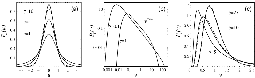
Figure 2: Distribution of the real $u$ and imaginary $v$ parts of the local Green function in the time-reversal chaotic cavity as absorption $\gamma$ grows. Dashed lines in (a) and (c) correspond to the limiting statistics (9joqaw) and (9joqau), respectively.

Along the same lines, we may consider the distribution $\mathcal{P}_{u}(u)$ of the real part $u$ (“reactance”). One finds from (9joqab)

$$\mathcal{P}_{u}(u)=\frac{1}{2\pi\sqrt{u^{2}+1}}\int_{0}^{\infty}\!\rmd q\,P_{0}\left[\frac{\sqrt{u^{2}+1}}{2}\Bigl{(}q+\frac{1}{q}\Bigr{)}\right]\,.$$ (9joqav)

The limiting forms of ${\mathcal{P}}_{u}(u)$ at weak and strong absorption follow readily as

$${\mathcal{P}}_{u}(u)\simeq\left\{\begin{array}[]{ll}\pi^{-1}(1+u^{2})^{-1}\,,&\alpha\ll 1\\[8.61108pt] \sqrt{\alpha/4\pi}\,e^{-\alpha u^{2}/4}\,,&\alpha\gg 1\end{array}\right.\,.$$ (9joqaw)

The Lorenzian distribution in the first line of (9joqaw) is the consequence of the uniform distribution of the scattering phase [90], as $u\approx\cot{\textstyle\frac{\theta}{2}}$ in the limit considered. As absorption grows, one can see the crossover to a Gaussian distribution centered at zero, which is again a result of the central limit theorem. This type of behavior as well as a trend of $\mathcal{P}_{v}(v)$ to the Gaussian distribution (9joqau), see figure 2, was recently observed in experiments on the cavity impedance [25, 26].

4.1.6 Delay time at vanishing absorption and eigenfunction intensity.

The Wigner’s time-delay is one of the most important and frequently used characteristics of quantum scattering. It was recently realized [35] that the fundamental relation (9joqab) allows one to relate the distribution of the time-delay $q$ in single-channel scattering (i.e. the Wigner’s time-delay) from a general lossless disordered system to the distribution of wave function intensities in the closed counterpart of such a system. Namely, consider the local eigenfunction intensity $y=\mathcal{V}|\psi_{n}({\bf r})|^{2}$ at a spatial point ${\bf r}$ of the closed system, with $\mathcal{V}$ denoting the volume of the sample and the index $n$ numbering different eigenfunctions. Let ${\cal P}_{y}(y)$ stand for the distribution of this intensity, where the statistics is sampled both over various realizations of the disorder in the system and over a certain small energy range around the point $E$ in the spectrum, with $\Delta$ being the mean level spacing in that energy range. Define the dimensionless time delay $\tau_{w}=q\Delta/2\pi$ corresponding to wave scattering at the chosen energy $E$ from a single channel attached to the point ${\bf r}$ of the sample. Denoting ${\cal P}_{w}(\tau_{w})$ the corresponding distribution in the regime of perfect coupling to the sample, Ossipov and Fyodorov managed to derive the following functional relation between the two distributions:

$$\mathcal{P}_{w}(\tau_{w})=\tau_{w}^{-3}\,\mathcal{P}_{y}(\tau_{w}^{-1})$$ (9joqax)

Referring the interested reader for the details of derivation to [35], we would like only to mention that at the starting point of the derivation the time delay is expressed via the reflection coefficient $r$ in presence of absorption: $\tau_{w}=\lim_{\gamma\to 0}\frac{1-r}{\gamma}$, see (6). Then one exploits in a clever way the scaling form of the distribution (9joqab) remembering both the interpretation of the variable $x$ in terms of $r$, see (9joqac), and the interpretation of $v$ as the LDoS, the latter step providing a connection to eigenfunction statistics.

On one hand, in the idealized situation of zero absorption statistics of delay times of all sorts were studied intensively in the framework of the RMT approach, various exact analytical results being available, see [40, 49, 83, 84, 91, 92, 93, 94, 95, 96] and references therein. Those were successfully verified in numerical simulations of chaotic systems of quite a diverse nature, see [97, 98, 99]. Since phase shifts and delay times are experimentally measurable quantities, especially in a single-channel reflection experiment [5, 8, 10, 100, 101, 102, 103], the relation (9joqax) opens a new possibility for experimental study of eigenfunctions.

On the other hand, one can use the existent knowledge on eigenfunction statistics [104, 29] to provide via (9joqax) explicit expressions for time-delay distributions. In this way one can e.g. recover those for chaotic systems of all symmetry classes obtained previously by diverse methods in various regimes of interest [40, 83, 84]. Of particular interest is the predicted multifractal behaviour of the negative moments of time-delays in the vicinity of the Anderson localisation transition [35]:

$$\left\langle\tau_{w}^{-q}\right\rangle\propto L^{-qD_{q+1}}$$ (9joqay)

where $L$ stands for the system size at criticality, and $D_{q}$ are anomalous (multifractal) dimensions of the eigenfunctions. Such a behaviour was indeed discovered recently [105] in numerical simulations of the disordered lattice Hamiltonians at criticality.

4.1.7 Anderson transition as phenomenon of spontaneous breakdown of S-matrix unitarity.

Actually, absorption in disordered systems plays not only purely technical, but also a conceptually important role in revealing the mechanisms behind the Anderson localisation transition. Lets us shortly discuss a possible qualitative behaviour of the PNR $\tau=1-r$ in a scattering system formed by a single perfect channel attached to a d-dimensional disordered sample at the vicinity of the point of the Anderson delocalisation transition $\mu_{c}$ (the mobility edge). Here we denote by $\mu$ an effective parameter which controls the transition in the infinite sample, with states being localised (extended) for $\mu>\mu_{c}$ (respectively, $\mu<\mu_{c}$).

For a sample of finite size $L$ the PNR is a function of three parameters: absorption $\Gamma$, size $L$, and disorder strength $\mu$. In the insulating phase $\mu>\mu_{c}$ the system is characterized by a localisation length $\xi$ which diverges when $\mu$ approaches the critical value. A natural scale for the absorption is played by a parameter $\delta\propto\Gamma\xi^{d}$ , i.e. the ratio of the imaginary shift in energy to the mean level spacing for sample of a typical size $L\propto\xi$ (localisation volume).

Consider the weak absorption limit $\delta\to 0$. It is clear that the wave incoming through the incident channel effectively explores only a part of the sample of the order of localisation volume $\xi^{d}$, being exponentially small elsewhere. Under this condition it is clear that the two limits: $\Gamma\to 0$ and $L\to\infty$ should actually commute and can be taken in arbitrary order. We know that in the limit $\Gamma\to 0$ the PNR behaves as $\tau\approx\Gamma q\to 0$, see (6). Moreover, exploiting the relation (9joqax), and remembering that $\langle|\psi_{n}({\bf r})|^{2k}\rangle\propto\xi^{-(k-1)d}$ it is easy to see that all negative integer PNR moments should behave in the infinite volume limit $L\to\infty$ as $\langle\tau^{-k}\rangle\sim\Gamma^{-k}\xi^{-dk}$. With a little bit more work one can suggest a qualitative picture for the PNR probability distribution in the localised phase. Namely, the distribution should have a powerlaw tail ${\cal P}(\tau)\propto\delta/\tau^{2}$ extending through a parametrically large domain $\delta<\tau<1$, and should decay very fast towards zero for both $\tau\ll\delta$ and $\tau\to 1$. When absorption vanishes $\delta\propto\Gamma\to 0$ such a distribution collapses to the Dirac $\delta-$function: $\mathcal{P}(\tau)\propto\delta(\tau)$, but in a very nonuniform way. We may conclude that in the limit of vanishing absorption $S$-matrix unitarity is indeed recovered, and in this sense we can associate the localised phase with the phase of unbroken symmetry.

In contrast, in the delocalized phase the incoming wave explores the whole sample volume. It is natural to think that whatever small (but fixed) is an absorption rate $\Gamma$, in the limit $L\to\infty$ a finite portion of the incoming flux will be absorbed in the sample and will never come back to the incident channel. In particular, we may expect $\lim_{\Gamma\to 0}\lim_{L\to\infty}\tau(\Gamma,L,\mu)=\tau_{\infty}(\mu)>0$ as long as $\mu<\mu_{c}$. From this point of view the Anderson transition acquires a natural interpretation as the phenomenon of spontaneous breakdown of $S$-matrix unitarity. Informal arguments in favour of such a behaviour are based on a picture of the transition as described in terms of a functional order parameter developed in detail in [81, 82], see also earlier results in [74] and [106]. Namely, the distribution function ${\cal P}(\tau)$ is expected to remain a non-trivial finite-width distribution even when $\Gamma\to 0$, provided the latter limit is taken after the infinite volume limit $L\to\infty$. Clearly, more work is needed to substantiate this claim, as well as to clarify critical behaviour of $\tau_{\infty}(\mu)$ as long as $\mu\to\mu_{c}$.

Note finally, that if the limit $\Gamma\to 0$ is taken first, then for $\mu<\mu_{c}$ PNR in large but finite sample should again scale with the system size $L$ as $\langle\tau^{-k}\rangle\sim C(\mu)\Gamma^{-k}L^{-dk}$, cf. (9joqay). The coefficient $C(\mu)$ is however expected to diverge when $\mu\to\mu_{c}$. This divergence should be related to the properties of eigenfunctions via equation (9joqax).

4.1.8 Arbitrary coupling to the channel.

The general case of arbitrary transmission coefficient, $T<1$, can be mapped [107, 108, 95, 10] to that of perfect coupling by making use of the following relation

$$S_{T=1}=\frac{S-\sqrt{1-T}}{1-\sqrt{1-T}S}$$ (9joqaz)

between the corresponding scattering matrices. Equation (9joqaz) is known from the Poisson kernel theory [107]. Due to an additional interference between incoming and directly back-scattered waves, the scattering phase $\theta$ acquires a non-uniform distribution and acquires statistical correlations with $x$ (or $r$). However, the joint probability density $P(x,\theta)$ is again determined by the function $P_{0}$ as follows [21] :

$$P(x,\theta)=\frac{1}{2\pi}P_{0}(xg-\sqrt{(x^{2}-1)(g^{2}-1)}\cos\theta)\,,\qquad g=\frac{2}{T}-1\geq 1$$ (9joqba)

This relation can be obtained by a straightforward evaluation in the parametrization (9joqaz) of the corresponding Jacobian. The integration over $x$ immediately yields the scattering phase distribution. In the particular case of vanishing absorption $r\to 1$ and $P_{0}(x)\to x^{-2}\delta(1/x)$. This readily gives $P(x,\theta)\to\rho(\theta)P_{0}(x)$, with the phase density $2\pi\rho(\theta)=(g-\sqrt{g^{2}-1}\cos\theta)^{-1}$ found earlier [95] (see [99] for the corresponding numerical study). As another example we consider the reflection coefficient distribution in terms of $P_{0}(x)$ is given at arbitrary $T$ by [17]:

$$P_{r}(r)=\frac{1}{\pi(1-r)^{2}}\int_{0}^{2\pi}\!\!\rmd\theta P_{0}\Bigl{[}\frac{2(g-\sqrt{g^{2}-1}\sqrt{r}\cos\theta)}{1-r}-g\Bigr{]}\,.$$ (9joqbb)

Distributions of $r$ and $\theta$ in microwave cavities were recently studied for different realizations of $\gamma$ and $T$ in [10], the excellent agreement with the theory being found.

4.2 Beyond single channel

4.2.1 Reflection coefficients and PNRs.

The starting point of our analysis in this section is the following convenient representation [17] for the diagonal elements $S^{cc}(E)$ of the scattering matrix, cf. (1):

$$S^{cc}(E)=\frac{1-\rmi K_{c}(E)}{1+\rmi K_{c}(E)}\,,\qquad K_{c}(E)={\textstyle\frac{1}{2}}V^{c{\dagger}}(E-\mathcal{H}_{\mathrm{eff}}^{c})^{-1}V^{c}\,.$$ (9joqbc)

where $\mathcal{H}_{\mathrm{eff}}^{c}=H-{\textstyle\frac{\rmi}{2}}\sum_{b\neq c}V^{b}V^{b{\dagger}}$ is now the $c-$dependent non-Hermitian operator. In view of $\mathcal{H}_{\mathrm{eff}}=H-\frac{i}{2}VV^{\dagger}\equiv\mathcal{H}_{\mathrm{eff}}^{c}-\frac{i}{2}V^{c}V^{c\dagger}$ one can treat $V^{c}V^{c\dagger}$ as a rank one perturbation with respect to $\mathcal{H}_{\mathrm{eff}}^{c}$. In this case the following general relationship (Dyson’s equation) is valid for the corresponding resolvents [38]:

$$\frac{1}{E-\mathcal{H}_{\mathrm{eff}}}=\frac{1}{E-\mathcal{H}_{\mathrm{eff}}^{c}}-\frac{\rmi}{2}\frac{1}{E-\mathcal{H}_{\mathrm{eff}}^{c}}V^{c}\frac{1}{1+\rmi K_{c}(E)}V^{c\dagger}\frac{1}{E-\mathcal{H}_{\mathrm{eff}}^{c}}$$ (9joqbd)

which can be proved by expanding the l.h.s. in a power series with respect to $(E-\mathcal{H}_{\mathrm{eff}}^{c})^{-1}V^{c}V^{c\dagger}$ and summing then up the resulting geometric series in $K_{c}$. Substituting this equation in $S^{cc}=1-\rmi V^{c\dagger}(E-\mathcal{H}_{\mathrm{eff}})^{-1}V^{c}$ one gets $S^{cc}=1-2\rmi K_{c}-2K_{c}(1+\rmi K_{c})^{-1}K_{c}$ which is equivalent to (9joqbc). It is also worth noting that a representation like (9joqbc) is valid for an arbitrary $m{\times}m$ submatrix standing on the main diagonal of $S$ with obvious replacement $V^{c}$ by the $N{\times}m$ matrix $V^{(m)}=(V^{c_{1}},\ldots,V^{c_{m}})$, and corresponding changes for $K_{c}$ and $\mathcal{H}_{\mathrm{eff}}^{c}$. In the particular case $m=M$, i.e. the full $S$-matrix, one recovers (1) from (2) and (9joqbd).

The relation (9joqbc) reduces the problem of evaluating the statistics of $S_{cc}$, and hence the reflection coefficient / PNR in a given channel $c$ to calculating the joint probability density $\mathcal{P}(u_{c},v_{c})$ of $u_{c}=\mathrm{Re\,}K_{c}$ and $v_{c}=-\mathrm{Im\,}K_{c}$, with $K_{c}$ standing for the particular diagonal entry of the resolvent of the effective non-Hermitian Hamiltonian $\mathcal{H}_{\mathrm{eff}}^{c}$ from (9joqbc). Moreover, a uniform absorption within the sample can again be taken into account by a purely imaginary shift of the scattering energy $E\to E+{\textstyle\frac{\rmi}{2}}\Gamma\equiv E_{\gamma}$, all further steps being fully in parallel to those of section 4.1.2. The most pleasant feature of this approach is that it is very straightforward to include open channels in the derivation of $\mathcal{P}(u_{c},v_{c})$ within the supersymmetry method. All important properties of this distribution, in particular, the relations (9joqab), (9joqao) and (9joqap) retain its validity, with $x$ being naturally replaced by $x_{c}={\textstyle\frac{1}{2v_{c}}}(u_{c}^{2}+v_{c}^{2}+1)$. The corresponding function $F(x_{c})$ then follows from (9joqao) by multiplying there the integrand with the “channel factor” (which originates from the imaginary part of $\mathcal{H}_{\mathrm{eff}}^{c}$)

$$\mathcal{F}_{M}^{c}(\{\lambda\})=\prod_{b\neq c}\left[\frac{(g_{b}+\lambda_{0})^{2}}{(g_{b}+\lambda_{1}\lambda_{2})-(\lambda_{1}^{2}-1)(\lambda_{2}^{2}-1)}\right]^{1/2},\qquad g_{b}=\frac{2}{T_{b}}-1$$ (9joqbe)

which accounts for arbitrary coupling to all other channels save for the given perfectly open one $c$. Arbitrary coupling for the remaining channel $c$ can be considered by means of (9joqba), providing us finally with the general distribution of the reflection amplitude and phase. In this way one can also obtain explicit distributions for many interesting situations [17], including the cases when the effects of Anderson localisation start to play an important role. In particular, in the case of broken TRS one can calculate the PNR distribution for a single channel attached to an edge of a piece of quasi-one-dimensional disordered medium of a given length $L$, with the opposite edge being either closed, or in contact with a perfectly conducting multichannel lead.

4.2.2 Reflection eigenvalues and thermal emission.

The exact result for the distribution function $P(r)$ of reflection eigenvalues valid for any number of arbitrary open channels and arbitrary absorption is known only for the $\beta=2$ case, being recently calculated by two of us [16], generalizing earlier perturbative results [15] (known for all $\beta$). That uses the method developed for studying the proper time-delay distribution [96] in the ideal lossless system. The later distribution considered at finite absorption by means of (6) has a sharp cutoff at $q=\Gamma^{-1}$ due to a finite value of $P(r)$ at $r=0$. This fact makes the interpretation of $q$ as delay times at strong absorption questionable [16], since intuitively one expects a generic exponential suppression at large values of delay times $q\gg\Gamma^{-1}$. Indeed, for the time $\delta t$ a wave-packet oscillating in the cavity with a frequency $\Delta/2\pi$ on average experiences $(\Delta/2\pi)\delta t$ collisions with the walls, yielding the probability $T_{\phi}(\Delta/2\pi)\delta t$ to be absorbed into one of $M_{\phi}$ parasitic channels ($T_{\phi}\ll 1$ being the transmission coefficient). The total reflection is then estimated as $R\simeq(1-T_{\phi}(\Delta/2\pi)\delta t)^{M_{\phi}}$, giving $e^{-\Gamma\delta t}$ in the absorption limit of the fixed absorption width $\Gamma=M_{\phi}T_{\phi}\Delta/2\pi$ as $M_{\phi}\to\infty$ and $T_{\phi}\to 0$. It is natural, therefore, to define alternatively the positive definite matrix $Q_{R}$ of reflection time-delays as follows [16]:

$$Q_{R}\equiv-\Gamma^{-1}\ln R_{\gamma}=-\Gamma^{-1}\ln(1-\Gamma Q_{\gamma})\,.$$ (9joqbf)

One finds easily the connection $\mathcal{P}_{R}(q_{r})=e^{-\Gamma q_{r}}\mathcal{P}[\frac{1}{\Gamma}(1-e^{-\Gamma q_{r}})]$ between the corresponding distributions $\mathcal{P}_{R}(q_{r})$ and $\mathcal{P}(q)$ of proper delay times (eigenvalues of $Q_{R}$ and $Q_{\gamma}$, respectively). Both $Q_{R}$ and $Q_{\gamma}$ reduce to the same Wigner-Smith matrix (4) in the limit of vanishing absorption. The difference between them becomes noticeable at finite $\Gamma$. Still both distributions coincide up to the time $\ll\Gamma^{-1}$. They start to differ at larger times, when $\mathcal{P}(q)$ has the cutoff whereas $\mathcal{P}_{R}(q\gg\Gamma^{-1})\propto e^{-\Gamma q}$ is exponentially suppressed.

The exact result for the $\beta=1$ case at arbitrary $M$ is still outstanding. In the limit of the large number of equivalent channels, $M\to\infty$, an exact result can be found at arbitrary absorption and coupling [18], and the perfect coupling case $T=1$ has been known for some time [109, 110]. In contrast to the few-channel case, when any value $0\leq r\leq 1$ is permitted, the distribution density in the present case is non-vanishing only in a range $0\leq r_{\mathrm{min}}\leq r\leq r_{\mathrm{max}}<1$, and is the same for all $\beta$. Referring the reader to [18] for explicit results, we mention their application for thermal emission from random media. Registration of $n$ photons in the frequency window $\delta\Omega$ during the large time $t\gg 1/\delta\Omega$ yields the negative-bimodal distribution of photocounts with $\nu=Mt\delta\Omega/2\pi$ degrees of freedom; see [111]. In his seminal paper Beenakker [109] has shown that the quantum optical problem of the photon statistics can be reduced to a computation of the $S$ matrix of the classical wave equation. In particular, chaotic radiation may be characterized by the effective number $\nu_{\mathrm{eff}}$ degrees of freedom as follows [109]: $\nu_{\mathrm{eff}}/\nu=(1-\langle{r}\rangle)^{2}/\langle(1-r)^{2}\rangle\leq 1$, with $\nu_{\mathrm{eff}}=\nu$ for blackbody radiation. This ratio is given by $\nu_{\mathrm{eff}}/\nu=(\gamma_{s}+T)^{2}/[\gamma_{s}^{2}+2(\gamma_{s}+T)]$ at arbitrary transmission $T$ and absorption $\gamma_{s}\equiv 2\pi\Gamma/\Delta M$, implying thus that saturation to the blackbody limit slows down, $\frac{\nu_{\mathrm{eff}}}{\nu}\approx 1-{\textstyle\frac{2}{\gamma}}_{s}(1-T)$ at $\gamma_{s}\gg 1$, for transmission $T<1$ [18]. Finally, due to a duality relation [109, 112] of a linear amplifying system to a dual absorbing one (related to it by inverting the sign of $\Gamma$) there exists a further link of the analysis presented here to the rapidly developing field of random lasers [109, 110, 112, 113, 114].

4.2.3 Off-diagonal entries of the Green function.

As we have seen, the statistics of real and imaginary parts of diagonal elements of the Green function can be very efficiently studied in the framework of the supersymmetric approach and may have various physical interpretations. The off-diagonal entries $G_{ij}(E_{\gamma})=\langle i|(E_{\gamma}-\mathcal{H}_{\mathrm{eff}})^{-1}|j\rangle$ are of considerable importance as well. It can be easily understood that $W=|G_{ij}|^{2}$ is essentially the wave power transmitted from a source at site $i$ inside a random medium to a receiver at site $j$. Statistics of such an object is much more difficult to study in general. Presently the most studied case [19] is $\beta=2$ symmetry class under an additional assumption that both receiver and source are very weakly coupled to the medium as to ensure those couplings do not contribute essentially to the resonance broadening. This means the broadening is induced purely due to losses elsewhere in the medium. Technically the latter requirement amounts to vanishing coupling amplitudes $V^{c}_{i}$ and $V^{c}_{j}$ for all damping channels $c=1\ldots M$. Assuming further the RMT statistics for $\mathrm{Re\,}\mathcal{H}_{\mathrm{eff}}$, it is easy to see that the damping matrix $\mathrm{Im\,}\mathcal{H}_{\mathrm{eff}}$ can be chosen diagonal and simply such that both entries $(VV^{\dagger})_{ii}$ and $(VV^{\dagger})_{jj}$ are vanishing. For such a model the distribution of the scaled transmitted power $w=({\textstyle\frac{\Delta}{\pi}})^{2}W$ can be found explicitly [19] as:

$${\cal P}(w)=\left(\frac{\rmd}{\rmd w}+w\frac{\rmd^{2}}{\rmd w^{2}}\right)\left[\frac{e^{-\gamma\sqrt{1+w}}}{2\sqrt{1+w}}\int_{-1}^{1}d\lambda\frac{\sqrt{1+w}+\lambda}{\sqrt{1+w}-\lambda}e^{\gamma\lambda}\prod_{c=1}^{M}\frac{g_{c}+\lambda}{g_{c}+\sqrt{1+w}}\right]\,.$$ (9joqbg)

In fact, the remaining integration can be performed for two interesting cases: (i) all equivalent dissipation channels $g_{c}=g$ in the absence of uniform losses $\gamma=0$ and (ii) no internal channels of dissipation $g_{c}\to\infty$ in the presence of uniform absorption $\gamma>0$. Here we present the formula only for the latter case [19]:

$$\mathcal{P}(w)=\frac{\gamma^{4}e^{-\gamma_{w}}\sinh{\gamma}}{4\gamma_{w}^{5}}\left[\gamma_{w}^{2}(w+2)-(w-2-2(\gamma_{w}^{2}/\gamma)\coth{\gamma})(1+\gamma_{w})\right]$$ (9joqbh)

with the shorthand $\gamma_{w}\equiv\gamma\sqrt{1+w}$. The distribution of the transmitted power for the case of absorptive media with preserved time-reversal invariance is not yet known. First two moments of that quantity were calculated recently in [20].

Let us finally mention that a closely related question of statistics of intensity of waves emitted from a permanently radiating source embedded in a random medium was the subject of many studies in recent years. Some useful references can be found in Section 7 of [29], see also the relevant review [114] on random lasing.

5 Conclusions and open problems

For wave scattering in open chaotic and/or disordered systems with uniform losses, we have discussed various statistics on the level of both correlation and distribution functions. The overall exponential decay due to uniform absorption is the generic feature of any correlation function reduced to a two-point spectral (resolvent) correlation function, that follows simply from analytic properties of the latter in the complex energy plane. For fully chaotic systems with or without TRS, we have calculated exactly energy correlation functions of complex impedance and $S$-matrix elements at arbitrary absorption and coupling. The corresponding enhancement factors have been also discussed in detail. The result for $S$-matrix correlations in the case of broken TRS completes the well known one [2] of preserved TRS.

To study distribution functions, we have described the novel approach to the problem by deriving a kind of a fluctuation dissipation relation (9joqaj) of quite a general nature, which relates distributions at finite absorption to arbitrary order correlations at zero absorption via a nontrivial analytic continuation procedure. Correlations can be efficiently studied in the framework of the supersymmetric nonlinear $\sigma$-model. In the zero dimensional case, a number of explicit results is provided for quantities characterizing open chaotic systems both from “inside” (LDoS, the complex impedance and the (local) Green’s function) and from “outside” (PNRs, reflection coefficients and time delays). This $\sigma$-model mapping provides an attractive possibility to include into consideration open disordered absorptive systems beyond the usual RMT treatment.

Finally, let us briefly discuss an (incomplete) list of problems deserving, from our personal point of view, further investigations both for scattering systems with and without absorption. Within the domain of RMT applicability, the most outstanding problems are of course those requiring evaluation of four-point correlation functions of the resolvents, e.g., partial scattering cross-sections. These are still not known even for the simplest case of broken TRS. Another challenge is to find a probability distribution for the multichannel $S$-matrix at finite absorption, thus nontrivially generalizing the Poisson kernel [90]. More work is required to understand an interplay between the statistics of complex resonances and the corresponding bi-orthogonal eigenfunctions [38, 69], the question being of particular relevance for lasing from random and/or chaotic media [115, 116]. Spatial characteristics of internal parts $b^{c}=(E-\mathcal{H}_{\mathrm{eff}})^{-1}V^{c}$ of the scattering wave function are very interesting by their own and are closely related to fluctuations in transmitted power discussed above in 4.2.3.

Apart from that, last decades it was realized [117] that it may be required to consider other symmetry classes (beyond the three of Dyson) which are relevant, e.g., for systems involving superconducting elements. The corresponding scattering theory is reviewed in [118]. To reconsider many problems discussed in the present review taking those (and other related) symmetries into account should be both interesting and informative (see [24] as a recent example).

At last but not least: understanding scattering in disordered systems beyond the universal RMT regime, taking into account, in particular, the effects of Anderson localisation, is a rather promising area calling for more systematic research.

Appendix A Statistics of the local Green function in the GSE

We start with expressing the dimensionless LDoS (the imaginary part of the local Green’s function $G(E+{\textstyle\frac{\rmi}{2}}\Gamma;{\bf r};{\bf r})$ in units of $\Delta$) in terms of the eigenfunctions and eigenvalues of the Hamiltonian $H$ with underlying simplectic symmetry as:

$$v({\bf r})=-\frac{\Delta}{\pi}\mbox{Im}\,G(E+{\textstyle\frac{\rmi}{2}}\Gamma;{\bf r},{\bf r})=\frac{\Delta}{\pi}\sum_{n=1}^{N}\left[|\psi_{n}({\bf r})|^{2}+|\phi_{n}({\bf r})|^{2}\right]\frac{\Gamma}{(E-E_{n})^{2}+{\textstyle\frac{1}{4}}\Gamma^{2}}\,.$$ (9joqbi)

Here $\psi_{n}({\bf r})$, $\phi_{n}({\bf r})$ stand for the local amplitudes of the two eigenfunctions corresponding to the (double-degenerate) eigenvalue $E_{n}$. It is convenient to consider scaled eigenvalues $\epsilon_{n}=\pi E_{n}/\Delta$, defining absorption $\eta=\pi\Gamma/\Delta\equiv{\textstyle\frac{1}{2}}\gamma$. Replacing $H$ with $2N\times 2N$ random GSE matrix, we follow the idea first suggested in [119] and in the first step exploit the well-known fact that in the limit $N\gg 1$ eigenvector components $\psi_{n}({\bf r}),\phi_{n}({\bf r})$ for different values of $n$ and ${\bf r}$ can be treated as independent, identically distributed complex Gaussian variables. The corresponding joint probability density can be written symbolically as ${\cal P}_{n}(\psi;\phi){\cal D}(\psi;\phi)=e^{-N(\psi^{\dagger}\psi+\phi^{\dagger}\phi)}{\cal D}(\psi;\phi)$ where we introduced a shorthand notation $\psi^{\dagger}\psi=\sum_{n=1}^{N}|\psi_{n}({\bf r})|^{2}$ (and similarly for $\phi^{\dagger}\phi$), with the measure ${\cal D}(\psi;\phi)$ being understood as the (normalized) product of differentials of independent variables.

The Laplace transform $F(s)=\int_{0}^{\infty}e^{-\rho s}\mathcal{P}_{\rho}(\rho)\rmd\rho$ of the probability distribution function ${\cal P}_{\rho}$ for the normalized variable $\rho=N\pi v({\bf r})$ can be then written as:

$$F(s)=\left\langle\int{\cal P}_{n}(\psi;\phi){\cal D}((\psi;\phi))\prod_{n=1}^{N}\exp{-\frac{sN\eta\left(|\psi_{n}({\bf r})|^{2}+|\phi_{n}({\bf r})|^{2}\right)}{(\epsilon-\epsilon_{n})^{2}+\eta^{2}}}\right\rangle_{\{\epsilon_{n}\}}$$ (9joqbj)

where the angular brackets stand for the averaging over the joint probability density of all eigenvalues $\epsilon_{n}$ and the limit $N\to\infty$ is to finally taken. After performing the Gaussian integrals, we therefore arrive to the following representation:

$$F(s)=\lim_{N\to\infty}\left\langle\prod_{n=1}^{N}\frac{\left[(\epsilon-\epsilon_{n})^{2}+\eta^{2}\right]^{2}}{\left[(\epsilon-\epsilon_{n})^{2}+\eta^{2}+2\eta s\right]^{2}}\right\rangle_{\{\epsilon_{n}\}}$$ (9joqbk)

Introducing the product $\pi_{N}(\lambda)=\prod_{n=1}^{N}\left(\lambda-\epsilon_{n}\right)$ we see that the characteristic polynomial of the GSE matrix $\hat{H}$ is simply $\pi^{2}_{N}(\lambda)$. The formula (9joqbk) can be conveniently rewritten in terms of this polynomial as:

$$F(s)=\lim_{N\to\infty}\left\langle\frac{\pi_{N}^{\beta/2}(\epsilon+\rmi\eta)\pi_{N}^{\beta/2}(\epsilon-\rmi\eta)}{\pi_{N}^{\beta/2}(\epsilon+\rmi\mu)\pi_{N}^{\beta/2}(\epsilon-\rmi\mu)}\right\rangle_{\{\epsilon_{n}\}},\quad\mu=\sqrt{\eta^{2}+2\eta s}$$ (9joqbl)

with $\beta=4$ for GSE. In fact, in such a form the formula retains its validity for GUE $\beta=2$ and GOE $\beta=1$ cases as well.

The problem of evaluating ensemble averages of products and ratios of characteristic polynomials of random matrices attracted a lot of research interest recently, both in physical and mathematical community. For $\beta=2$, the general problem was solved in [120, 121], and the most complete set of formulae available presently for $\beta=1,4$ can be found in the recent paper by Borodin and Strahov [122]. When addressing the most interesting case $\beta=1$ they were, unfortunately, able to consider only integer powers of characteristic polynomials, whereas (9joqbl) obviously requires knowledge of half-integer powers. In this sense the corresponding random matrix problem for $\beta=1$ case is still outstanding. Borodin and Strahov derived the following explicit expression for the $\beta=4$ average featuring in (9joqbl):

$$\lim_{N\to\infty}\left\langle\frac{\pi_{N}^{2}(\alpha_{1})\pi_{N}^{2}(\alpha_{2})}{\pi_{N}^{2}(\beta_{1})\pi_{N}^{2}(\beta_{2})}\right\rangle_{GSE}=\frac{\prod_{i,j=1}^{2}(\alpha_{i}-\beta_{j})}{(\alpha_{1}-\alpha_{2})(\beta_{1}-\beta_{2})}\,\,\mbox{Pf}\,\hat{C}$$ (9joqbm)

assuming that $\mbox{Im}{\beta_{1}}>0,\,\mbox{Im}{\beta_{2}}<0$. Here, the matrix $\hat{C}$ has the following structure $\scriptsize\hat{C}=\left(\begin{array}[]{cc}\hat{A}&\hat{B}\\ -\hat{B}^{T}&\hat{D}\end{array}\right)$, with $\scriptsize\hat{A}=\left(\begin{array}[]{cc}0&a\\ -a&0\end{array}\right)$, $\scriptsize\hat{D}=\left(\begin{array}[]{cc}0&d\\ -d&0\end{array}\right)$, $\scriptsize\hat{B}=\left(\begin{array}[]{cc}b_{11}&b_{12}\\ b_{21}&b_{22}\end{array}\right)$ and Pf stands for the corresponding Pfaffian, $\mbox{Pf}\,\hat{C}=\sqrt{\mbox{det}\,\hat{C}}$. The entries of the matrix $\hat{C}$ are given explicitly by:

$$a=\frac{1}{\pi}\int_{0}^{1}\frac{\rmd t}{t}\sin{(\alpha_{1}-\alpha_{2})t},\qquad d=2\pi\rmi\frac{\partial}{\partial\beta_{1}}\left(\frac{e^{\rmi(\beta_{1}-\beta_{2})}}{\beta_{1}-\beta_{2}}\right)$$ (9joqbn)

$$b_{11}=-\frac{e^{\rmi(\beta_{1}-\alpha_{1})}}{\beta_{1}-\alpha_{1}},\quad b_{12}=\frac{e^{\rmi(\alpha_{1}-\beta_{2})}}{\alpha_{1}-\beta_{2}},\quad b_{21}=-\frac{e^{\rmi(\beta_{1}-\alpha_{2})}}{\beta_{1}-\alpha_{2}},\quad b_{22}=\frac{e^{\rmi(\alpha_{2}-\beta_{2})}}{\alpha_{2}-\beta_{2}}$$ (9joqbo)

Restricting our consideration in (9joqbl) for simplicity to $\epsilon=E=0$ we have therefore $\alpha_{1}=\rmi\eta,\alpha_{2}=-\rmi\eta,\beta_{1}=\rmi\mu,\beta_{2}=-\rmi\mu$. Substituting this to (9joqbn)–(9joqbo) and then to (9joqbm), we find after straightforward computations the Laplace transform of the LDoS probability density:

$$F_{GSE}(s)=F_{GUE}(s)+\delta F(s),$$ (9joqbp)

$$F_{GUE}(s)=\frac{1}{4\eta\mu}\left(e^{-2(\eta-\mu)}(\eta+\mu)^{2}-e^{-2(\eta+\mu)}(\eta-\mu)^{2}\right)$$ (9joqbq)

$$\delta F(s)=\frac{1}{4\eta\mu^{2}}(\eta^{2}-\mu^{2})^{2}e^{-2\eta}\left(1+\frac{1}{2\mu}\right)\int_{0}^{1}\frac{\rmd t}{t}\sinh{(2\eta t)},$$ (9joqbr)

We note that (i) the only $s-$dependence in the above expression comes from $\mu=\sqrt{\eta^{2}+2\eta s}$ and (ii) the formula (9joqbq) concides with the Laplace transform of the LDoS distributuion for $\beta=2$ case, see e.g. [88, 119].

The remaining job is to find the part $\delta F(\rho)$ of the LDoS probability density corresponding to inversion of the Laplace transform in (9joqbr), which gives

$$\delta F(\rho)=\frac{\rmd^{2}}{\rmd\rho^{2}}\left[\rho^{1/2}e^{-\eta(\rho/2+2/\rho)}\right]\times\frac{1}{4}\sqrt{\frac{2}{\pi\eta}}\int_{0}^{1}\frac{\rmd t}{t}\sinh{(2\eta t)}$$ (9joqbs)

Knowledge of this function allows immediate restoration of the corresponding probability density (9joqaf) for the main scaling variable $x$ due to relations discussed in the main body of the present paper (recall that $\eta=\gamma/2$).

Appendix B Disordered systems of arbitrary dimension:
nonlinear $\sigma$-model derivation of expressions (9joqak)

Let $\mathbb{H}$ be a (self-adjoint) Hamiltonian describing a one-particle quantum motion in a d-dimensional static disordered potential. Among microscopic model Hamiltonians ensuring validity of the non-linear sigma-model description of such a system the simplest choice seems to be the Wegner’s $N-$orbital model [123, 124], or its variant due to Pruisken and Schäfer [125]. Physically the models are equivalent to the so-called “granulated metal” model [74]. One can visualize it by considering a lattice of $L^{d}$ sites ($d$ standing for the spatial dimension of the sample) , each site being occupied with a metallic “granula”. The motion of a quantum particle inside each granula is assumed to be fully ”ergodic”, and as such the Hamiltonian of the individual granula should be adequately modelled by a random $N\times N$ matrix $\hat{H}$ of appropriate symmetry, provided we consider the limit $N\to\infty$. The quantum particle is also allowed to tunnel between the neighbouring granulae, the process ensuring a possibility of nontrivial diffusive motion along the lattice. Thus, the Hamiltonian $\mathbb{H}$ of the system as a whole has a form of large matrix of the size $N\times L^{d}$, consisting of coupled matrix blocks $\hat{H}_{k},\,\,k=1,2,\ldots,L^{d}$ of the size $N\times N$. For example, for the simplest quasi-one dimensional sample $d=1$ such a matrix will be “block-three-diagonal”.

Being interested in scattering, we should provide a way to incorporate description of external leads (or waveguides) attached to the sample. In the framework of the present model attaching an $M_{k}$-channel lead to the block at site $k$ is done by replacing the corresponding “intragranula” matrix block $\hat{H}_{k},$ with its non-selfadjoint counterpart $\hat{H}_{k}-{\textstyle\frac{\rmi}{2}}\hat{\Gamma}_{k}$, where $N\times N$ matrix $\hat{\Gamma}_{k}=2\,\mbox{diag}(\kappa_{1}^{(k)},\ldots,\kappa_{M_{k}}^{(k)},0,\ldots,0)\geq 0$, and $M_{k}$ staying finite when $N\to\infty$. Assuming the absorption width $\Gamma$ to be uniform and identical in all the granulae, we are interested in deriving the joint probability density ${\cal P}(u,v)$ of real $u$ and imaginary $v$ parts of the local Green’s function in a state $|j^{(l)}\rangle$ belonging to granule at the lattice site $l$:

$$G(j^{(l)},j^{(l)},E_{\gamma})=\langle j^{(l)}|(E_{\gamma}-\mathbb{H}+{\textstyle\frac{\rmi}{2}}\hat{\Gamma})^{-1}|j^{(l)}\rangle\,.$$ (9joqbt)

Following the general strategy (see Section 4.1.2) we recover $\mathcal{P}(u,v)$ from the correlation function $C(z^{\prime},z^{\prime\prime})$, see (4.1.2). The calculation of the corresponding correlation function is a straightforward extension of the “zero-dimensional” procedure employed in [40] for $\beta=2$ and then in [84] for $\beta=1$ (as well as for the whole crossover) to the present d-dimensional situation and will not be repeated here. The emerging supersymmetric nonlinear $\sigma$-model on the lattice is described in terms of the supermatrices $Q_{k},\,k=1,\ldots L^{d}$ parametrized as $Q_{k}=-\rmi\hat{T}_{k}\Lambda\hat{T}_{k}^{-1}$ and interacting according to the “action” (see e.g. [81])

$$S\{Q\}=-\frac{t\beta}{4}\sum_{<k,j>}^{L^{d}}\mbox{Str}\,\,Q_{k}Q_{j}+\frac{\beta}{4}\frac{\Gamma}{\Delta}\sum_{k}^{L^{d}}\mbox{Str}\,\,Q_{k}\Lambda$$ (9joqbu)

where the first sum goes over pairs $<k,j>$ of nearest neighbours on the underlying lattice, $\Delta$ stands for the mean level spacing and $t$ stands for the effective inter-granule coupling constant, which is the main control parameter of the emerging theory. We start with outlining the procedure for $\beta=2$ symmetry when $Q$-matrices involved in the calculation have the smallest size $4{\times}4$. Assuming for simplicity that the granule $l$ does not have a channel attached to it directly, the correlation function $C(z^{\prime},z^{\prime\prime})$, see (9joqag) and (4.1.2), of resolvents of the (scaled with ${\textstyle\frac{N\Delta}{\pi}}$) Green’s functions (9joqbt) is expressed in terms of the $Q$-integrals as follows

$$C_{\beta=2}(z^{\prime},z^{\prime\prime})=\prod^{L^{d}}_{k=1}\int\rmd\mu(Q_{k})\,\mathcal{F}^{(k)}_{M_{k}}(Q_{k})\,e^{-S\{Q\}}{\textstyle\frac{\partial^{2}}{\partial J_{1}\partial J_{2}}}\mbox{Sdet}^{-1}(U_{J}^{-1}+Q_{l})\big{|}_{J_{1}=J_{2}=0}$$ (9joqbv)

where the supermatrix $U$ depends on the variables $z^{\prime},z^{\prime\prime}$ and sources $J_{1},J_{2}$ via

$$U={\textstyle\frac{1}{2}}(z^{\prime}-iz^{\prime\prime})(1+\Lambda)+{\textstyle\frac{1}{2}}(z^{\prime}+\rmi z^{\prime\prime})(1-\Lambda)+\mbox{diag}(0,J_{1},0,J_{2})\,.$$ (9joqbw)

The “channel factor” $\mathcal{F}^{(k)}_{M_{k}}(Q_{k})\equiv\prod_{c=1}^{M_{k}}\mbox{Sdet}^{-1}(1+\rmi\kappa_{c}^{(k)}Q_{k}\Lambda)$ originates from coupling to continuum, where $\kappa^{(k)}=0$ if no external channels is attached to a given granule. The factors $\mathcal{F}_{M}$ appearing explicitly in Section 3.2 as well as in (9joqbe) are just the zero-dimensional analogue of $\mathcal{F}^{(k)}_{M_{k}}$. Following [81, 82], we find it convenient to introduce the function

$$Y^{(l)}(Q_{l})=\prod^{L^{d}}_{k\neq l}\int\rmd\mu(Q_{k})\,\mathcal{F}^{(k)}_{M_{k}}(Q_{k})\,e^{-S\{Q\}}\,.$$ (9joqbx)

Employing the standard Efetov-type parametrization of the matrices $Q$, one finds that actually $Y^{(l)}(Q)$ must be a function of only two commuting variables: $1\leq\lambda_{1}\leq\infty$ and $-1\leq\lambda_{0}\leq 1$. Then integrating out all the remaining degrees of freedom in quite a standard way (see [40] for more detail), we arrive at the representation (9joqak) where

$$\mathcal{F}_{\beta=2}(z^{\prime},z^{\prime\prime})=\int_{1}^{\infty}\rmd\lambda_{1}\int_{-1}^{1}\frac{\rmd\lambda_{0}}{(\lambda_{1}-\lambda_{0})^{2}}\frac{\tilde{x}+\lambda_{0}}{\tilde{x}+\lambda_{1}}\,Y^{(l)}(\lambda_{1},\lambda_{0})$$ (9joqby)

the main scaling variable of our theory $\tilde{x}\equiv{\textstyle\frac{1}{2z^{\prime\prime}}}(z^{\prime 2}+z^{\prime\prime 2}+1)$ being introduced. This immediately verifies the structure of the important formula (9joqak) for a general d-dimensional $\beta=2$ system with attached scattering channels. Of course, ability to work out explicit expressions for the probability density ${\cal P}(u,v)$ crucially depends on the availability of the function $Y^{(l)}(\lambda_{1},\lambda)$. This function has a very simple form in ”zero dimension”, physically equivalent to a system consisting of a single granula:

$$Y^{(l)}(\lambda_{1},\lambda_{0})=e^{-\gamma(\lambda_{1}-\lambda_{0})/2}\prod_{c=1}^{M}\frac{g_{c}+\lambda_{0}}{g_{c}+\lambda_{1}}$$ (9joqbz)

where we have assumed that the total number of external channels attached to the system is $M$. Each channel is characterised by its own effective coupling constant $g_{c}=\frac{1}{2}(\kappa_{c}+\kappa_{c}^{-1})\geq 1$, the transmission coefficient being $T_{c}={\textstyle\frac{2}{g_{c}+1}}$. Weak-localisation corrections to zero dimensional results can be in principle found systematically following the procedures of [104], and non-perturbative results are mainly available in quasi-1D systems, see e.g. [126], in the limit of weak absorption, $\gamma\ll 1$.

Treating systems of $\beta=1$ symmetry class follows exactly the same steps as outlined before, although in this case the supermatrices $Q$ are of the size $8{\times}8$ with the corresponding doubling the dimension of (9joqbw). Following [84, 86], we consider the whole crossover between $\beta=1$ and $\beta=2$ symmetry classes. Due to the TRS breaking perturbation controlled by the parameter $y$ ($\hat{H}_{k}$ is no longer symmetric but still Hermitian), the action (9joqbu) (with $\beta=1$) acquires additionally the symmetry breaking term $S_{y}\{Q\}={\textstyle\frac{1}{4}}y^{2}\sum_{k}\mbox{Str}\,(\tau_{3}Q_{k})^{2}$, with $\tau_{3}$ being the Pauli matrix. As usual, explicit integrations are much more cumbersome and require more work, some very useful and helpful relations can be found in [86]. Exploiting the parametrization suggested there, the function $Y^{(l)}(Q)$ turns out again to be dependent on three variables $1\leq\lambda_{1,2}\leq\infty$ and $-1\leq\lambda_{0}\leq 1$, and the analogue of (9joqby) reads

$$\mathcal{F}_{\beta=1}(z^{\prime},z^{\prime\prime})=\int_{1}^{\infty}d\lambda_{1}\int_{1}^{\infty}\rmd\lambda_{2}\int_{-1}^{1}\frac{\rmd\lambda_{0}}{\mathcal{R}^{2}}\,\frac{\tilde{x}+\lambda_{0}}{\sqrt{(\tilde{x}+\tilde{\mu}_{1})(\tilde{x}+\tilde{\mu}_{2})}}\,\,\,Y^{(l)}(\lambda_{1},\lambda_{2},\lambda_{0})$$ (9joqca)

where $\mathcal{R}=\lambda_{0}^{2}+\lambda_{1}^{2}+\lambda_{2}^{2}-2\lambda_{0}\lambda_{1}\lambda_{2}-1$ and $\tilde{\mu}_{1,2}=\lambda_{1}\lambda_{2}\pm\sqrt{(\lambda_{1}^{2}-1)(\lambda_{2}^{2}-1)}$, and in zero dimension:

$$Y^{(l)}(\lambda_{1},\lambda_{2},\lambda_{0})=f(\{\lambda\})e^{-\gamma(\lambda_{1}\lambda_{2}-\lambda_{0})/2}\prod_{c=1}^{M}\frac{g_{c}+\lambda_{0}}{\sqrt{(g_{c}+\tilde{\mu}_{1})(g_{c}+\tilde{\mu}_{2})}}\,.$$ (9joqcb)

Here, $f(\{\lambda\})$ coming solely due to the $e^{-S_{y}\{Q\}}$ term is explicitly given by (4.1.2). Integration variables $\tilde{\mu}_{1,2}$ make a connection between the “radial” parametrisation of $Q$ of [72] and the “angular” parametrisation of [2]. This will be utilised in the next Appendix to get explicit result for the zero-dimensional case for $\beta=1$.

Appendix C Analytic continuation (9joqan) and GOE result (9joqar)

We prove here equivalence of the analytic continuation of the “connected” part of $C(z^{\prime},z^{\prime\prime})$ in $z^{\prime\prime}\to-v\pm\rmi 0$ (9joqaj) to that of $\mathcal{F}(\tilde{x})$ in $\tilde{x}\to-x\pm\rmi 0$ (9joqan). Let us consider in detail first the simplest case of $\beta=2$ symmetry class in zero dimension. Then

$$C(z^{\prime},z^{\prime\prime})=\frac{1}{z^{\prime 2}+(z^{\prime\prime}+1)^{2}}-\frac{1}{4}\left(\frac{\partial^{2}}{\partial z^{\prime 2}}\!+\!\frac{\partial^{2}}{\partial z^{\prime\prime 2}}\right)$$

$$\times\int_{1}^{\infty}\rmd\lambda_{1}\int_{-1}^{1}\frac{\rmd\lambda_{0}}{\lambda_{1}-\lambda_{0}}\frac{2z^{\prime\prime}e^{-\gamma(\lambda_{1}-\lambda_{0})/2}}{z^{\prime 2}+z^{\prime\prime 2}+2z^{\prime\prime}\lambda_{1}+1}$$ (9joqcc)

where we have kept in the integrand only the term remaining nonzero under the differentiation. The FT $\hat{C}(k,z^{\prime\prime})$ with respect to the first argument reads as follows:

$$\widehat{C}(k,z^{\prime\prime})=\frac{\pi e^{-|k|(z^{\prime\prime}+1)}}{z^{\prime\prime}+1}-\frac{1}{4}\left(-k^{2}\!+\!\frac{\partial^{2}}{\partial z^{\prime\prime 2}}\right)$$

$$\times\int_{1}^{\infty}\rmd\lambda_{1}\int_{-1}^{1}\frac{\rmd\lambda_{0}}{\lambda_{1}-\lambda_{0}}\frac{\pi e^{-|k|\sqrt{z^{\prime\prime 2}+2z^{\prime\prime}\lambda_{1}+1}}}{\sqrt{z^{\prime\prime 2}+2z^{\prime\prime}\lambda_{1}+1}}2z^{\prime\prime}e^{-\gamma(\lambda_{1}-\lambda_{0})/2}\,.$$ (9joqcd)

Now we continue this result analytically in $z^{\prime\prime}$ and calculate the jump (9joqaj) on the negative real axis $z^{\prime\prime}\to-v\pm\rmi 0$, with $v>0$. One gets readily

$$\widehat{\mathcal{P}}(k,v)=\delta(v-1)+\frac{1}{2\pi}\left(-k^{2}\!+\!\frac{\partial^{2}}{\partial v^{2}}\right)$$

$$\times\int_{{\textstyle\frac{1+v^{2}}{2v}}}^{\infty}\rmd\lambda_{1}\int_{-1}^{1}\frac{\rmd\lambda_{0}}{\lambda_{1}-\lambda_{0}}\frac{\cos(k\sqrt{2v\lambda_{1}-1-v^{2}})}{\sqrt{2v\lambda_{1}-1-v^{2}}}v\,e^{-\gamma(\lambda_{1}-\lambda_{0})/2}\,.$$ (9joqce)

Performing now the inverse FT one arrives at

$$\mathcal{P}(u,v)=\delta(u)\delta(v-1)+\frac{1}{4\pi}\left(\frac{\partial^{2}}{\partial u^{2}}\!+\!\frac{\partial^{2}}{\partial v^{2}}\right)$$

$$\times\int_{{\textstyle\frac{1+v^{2}}{2v}}}^{\infty}\rmd\lambda_{1}\int_{-1}^{1}\frac{\rmd\lambda_{0}}{\lambda_{1}-\lambda_{0}}e^{-\gamma(\lambda_{1}-\lambda_{0})/2}\delta(u^{2}+v^{2}+1-2v\lambda_{1})\,2v\,.$$ (9joqcf)

Making now use of $\delta(u^{2}+v^{2}+1-2v\lambda_{1})\,2v={\textstyle\frac{\partial}{\partial\lambda_{1}}}\Theta(2\lambda_{1}v-u^{2}-v^{2}-1)=\delta(\lambda_{1}-x)$, with $x={\textstyle\frac{1}{2v}}(u^{2}+v^{2}+1)$ from (9joqab), one can immediately integrate (C) over $\lambda_{1}$, yielding $\int_{x-1}^{x+1}\rmd t\,t^{-1}e^{-\gamma t/2}$ for the second line, that is in exact agreement with expression (9joqaq) following from the analytic continuation (9joqan).

The proof for the $\beta=1$ case proceeds along the same lines, explicit expressions being however more lengthy. We omit it, considering instead the less trivial derivation of expression (9joqar). It is important to stress that for $\beta=1$ the nonzero $F(x)$ (9joqao) at given $x>1$ is determined by the integration region $\mathcal{B}_{x}=\{(\tilde{\mu}_{1},\tilde{\mu}_{2})\,|\,x\leq\tilde{\mu}_{1}<\infty,\,0\leq\tilde{\mu}_{2}\leq x\}$, rather than by a single point $\lambda_{1}=x$ as in the $\beta=2$ case. It is convenient, therefore, to choose $\tilde{\mu}_{1,2}$ from (9joqca) as new integration variables. Actually, they are related to those from [2] (which are already used in (9jop)) as follows:

$$\mu_{1,2}={\textstyle\frac{1}{2}}(\tilde{\mu}_{1,2}-1)\equiv{\textstyle\frac{1}{2}}\left[\lambda_{1}\lambda_{2}\pm\sqrt{(\lambda_{1}^{2}-1)(\lambda_{2}^{2}-1)}\right]\,,\qquad\mu_{0}={\textstyle\frac{1}{2}}(1-\lambda_{0})\,.$$ (9joqcg)

with the pre-exponential factor in (9jop) being the corresponding integration measure. Expression (9joqao) at $y=0$ acquires then the following form (with $w\equiv\frac{x-1}{2}$):

$$F(x)=\int_{0}^{1}\!\rmd\mu_{0}\int_{w}^{\infty}\!\rmd\mu_{1}\!\int_{0}^{w}\!\frac{\rmd\mu_{2}\,\,(1-\mu_{0})\mu_{0}(\mu_{1}-\mu_{2})}{\sqrt{\mu_{1}(1+\mu_{1})\mu_{2}(1+\mu_{2})}(\mu_{0}+\mu_{1})^{2}(\mu_{0}+\mu_{2})^{2}}$$

$$\times e^{-\gamma(\mu_{1}+\mu_{2}+2\mu_{0})/2}\frac{w+\mu_{0}}{\sqrt{(\mu_{1}-w)(w-\mu_{2})}}$$

$$\hbox to0.0pt{\hss${}={}$}\int_{0}^{1/w}\!\!\rmd\nu_{0}\int_{1}^{\infty}\!\rmd\nu_{1}\!\int_{0}^{1}\!\frac{\rmd\nu_{2}\,\,(1+\nu_{0})\nu_{0}(\nu_{1}-\nu_{2})}{\sqrt{\nu_{1}(\nu_{1}-1)\nu_{2}(\nu_{2}-1)}(\nu_{0}+\nu_{1})^{2}(\nu_{0}+\nu_{2})^{2}}$$

$$\times e^{-\gamma w(\nu_{1}+\nu_{2}+2\nu_{0})/2}\frac{1-w\nu_{0}}{\sqrt{(1+w\nu_{1})(1+w\nu_{2})}}$$ (9joqch)

where the second equality comes after the scaling $\mu_{0,1,2}=w\,\nu_{0,1,2}$. It is convenient to consider now the function $\frac{\rmd}{\rmd x}F(x)$. An essential observation is that this function contains no contribution coming from the derivative of (C) on the upper limit due to vanishing of the integrand at $\nu_{0}=0,{\textstyle\frac{1}{w}}$. We represent it in the following form:

$$\frac{\rmd F(x)}{\rmd x}=\int_{0}^{1/w}\!\!\rmd\nu_{0}\int_{1}^{\infty}\!\rmd\nu_{1}\!\int_{0}^{1}\!\frac{\rmd\nu_{2}\,\,e^{-\gamma w(\nu_{1}+\nu_{2}+2\nu_{0})/2}\,X(\nu_{0},\nu_{1},\nu_{2})}{\sqrt{\nu_{1}(\nu_{1}-1)\nu_{2}(\nu_{2}-1)(1+w\nu_{1})(1+w\nu_{2})}}$$ (9joqci)

where a rational function $X$ contains all other terms resulting from the differentiation. It is a crucial fact that $X$ can be further decomposed into partial fractions with respect to $\nu_{0}$, yielding

$$X(\nu_{0},\nu_{1},\nu_{2})=\sum_{i=1,2}(-1)^{i+1}\left[\frac{a_{i}(\gamma+d_{12})}{(\nu_{0}+\nu_{i})^{2}}+\frac{\gamma b_{i}+c_{i}d_{12}}{\nu_{0}+\nu_{i}}+2w\gamma\nu_{i}\right]$$ (9joqcj)

with functions $a_{i}=\nu_{i}(\nu_{i}-1)(1+w\nu_{i})$, $b_{i}=1-2(1-w)\nu_{i}-3w\nu_{i}^{2}$, $c_{i}=1-2\nu_{i}-w\nu_{i}^{2}$ for $i=1,2$ and $d_{12}=[(1+w\nu_{1})(1+w\nu_{2})]^{-1}$. Substituting (9joqcj) in (9joqci), one readily sees that integrals over $\nu_{0}$ can be easily performed while remaining integrations over $\nu_{1,2}$ get completely decoupled in each term of the sum, leading finally to (9joqar).

References

- [1] Stöckmann H J 1999 Quantum Chaos: An Introduction (Cambridge, UK: Cambridge University Press)
- [2] Verbaarschot J J M, Weidenmüller H A and Zirnbauer M R 1985 Phys. Rep. 129 367
- [3] Beenakker C W J 1997 Rev. Mod. Phys. 69 731
- [4] Alhassid Y 2000 Rev. Mod. Phys. 72 895
- [5] Doron E, Smilansky U and Frenkel A 1990 Phys. Rev. Lett. 65 3072
- [6] Lewenkopf C H, Müller A and Doron E 1992 Phys. Rev. A 45 2635
- [7] Schäfer R, Gorin T, Seligman T H and Stöckmann H J 2003 J. Phys. A: Math. Gen. 36 3289
- [8] Méndez-Sánchez R A, Kuhl U, Barth M, Lewenkopf C H and Stöckmann H J 2003 Phys. Rev. Lett. 91 174102
- [9] Schanze H, Stöckmann H J, Martínez-Mares M and Lewenkopf C H 2005 Phys. Rev. E 71 016223
- [10] Kuhl U, Martínez-Mares M, Méndez-Sánchez R A and Stöckmann H J 2005 Phys. Rev. Lett. 94 144101
- [11] Barthélemy J, Legrand O and Mortessagne F 2005 Europhys. Lett. 70 162
- [12] Lobkis O I, Rozhkov I S and Weaver R L 2003 Phys. Rev. Lett. 91 194101
- [13] Hul O, Bauch S, Pakonski P, Savytskyy N, Zyczkowski K and Sirko L 2004 Phys. Rev. E 69 056205
- [14] Kogan E, Mello P A and Liqun H 2000 Phys. Rev. E 61 R17
- [15] Beenakker C W J and Brouwer P W 2001 Physica E 9 463
- [16] Savin D V and Sommers H J 2003 Phys. Rev. E 68 036211
- [17] Fyodorov Y V 2003 JETP Lett. 78 250
- [18] Savin D V and Sommers H J 2004 Phys. Rev. E 69 035201(R)
- [19] Rozhkov I, Fyodorov Y V and Weaver R L 2003 Phys. Rev. E 68 016204
- [20] Rozhkov I, Fyodorov Y V and Weaver R L 2004 Phys. Rev. E 69 036206
- [21] Fyodorov Y V and Savin D V 2004 JETP Lett. 80 725
- [22] Savin D V, Sommers H J and Fyodorov Y V 2005 JETP Lett. 82 544 (cond–mat/0502359)
- [23] Martinez-Mares M and Mello P A 2005 Phys. Rev. E 72 026224
- [24] Fyodorov Y V and Ossipov A 2004 Phys. Rev. Lett. 92 084103
- [25] Hemmady S, Zheng X, Ott E, Antonsen T M and Anlage S M 2005 Phys. Rev. Lett. 94 014102
- [26] Hemmady S, Zheng X, Antonsen T M, Ott E and Anlage S M 2005 Phys. Rev. E 71 056215
- [27] Zheng X, Antonsen T M and Ott E 2004 e-print cond–mat/0408327
- [28] Zheng X, Antonsen T M and Ott E 2004 e-print cond–mat/0408317
- [29] Mirlin A D 2000 Phys. Rep. 326 259
- [30] Fyodorov Y V and Alhassid Y 1998 Phys. Rev. A 58 R3375
- [31] Sokolov V V, Rotter I, Savin D V and Müller M 1997 Phys. Rev. C 56 1044
- [32] Gorin T, Mehlig B and Ihra W 2004 J. Phys. A: Math. Gen. 37 L345
- [33] Misirpashaev T Sh, Brouwer P W and Beenakker C W J 1997 Phys. Rev. Lett. 79 1841
- [34] Savin D V, Fyodorov Y V and Sommers H J 2005 e-print nlin.CD/0506040
- [35] Ossipov A and Fyodorov Y V 2005 Phys. Rev. B 71 125133
-
[36]
Livšic M S 1957 Sov. Phys. JETP
4 91
Livšic M S 1973 Operators, Oscillations, Waves (Open Systems), Transl. Math. Monographs, Vol. 34 (RI, Providence: American Mathematical Society) - [37] Mahaux C and Weidenmüller H A 1969 Shell-model Approach to Nuclear Reactions (Amsterdam: North-Holland)
- [38] Sokolov V V and Zelevinsky V G 1989 Nucl. Phys. A 504 562
- [39] Lewenkopf C H and Weidenmüller H A 1991 Ann. Phys. (N.Y.) 212 53
- [40] Fyodorov Y V and Sommers H J 1997 J. Math. Phys. 38 1918
- [41] Dittes F M 2000 Phys. Rep. 339 215
- [42] Nussenzveig H M 1972 Causality and Dispersion Relations (New York: Academic Press)
- [43] Pichugin K, Schanz H and Šeba P 2001 Phys. Rev. E 64 056227
- [44] Stöckmann H J, Persson E, Kim Y H, Barth M, Kuhl U and Rotter I 2002 Phys. Rev. E 65 066211
- [45] Savin D V, Sokolov V V and Sommers H J 2003 Phys. Rev. E 67 026215
- [46] Barthélemy J, Legrand O and Mortessagne F 2005 Phys. Rev. E 71 016205
- [47] Wigner E 1955 Phys. Rev. 98 145
- [48] Smith F T 1960 Phys. Rev. 118 349
- [49] Lehmann N, Savin D V, Sokolov V V and Sommers H J 1995 Physica D 86 572
- [50] Sokolov V V and Zelevinsky V 1997 Phys. Rev. C 56 311
- [51] Lyuboshitz V L 1977 Phys. Lett. B 72 41
- [52] Muga J G and Leavens C R 2000 Phys. Rep. 338 353
- [53] de Carvalho C A A and Nussenzveig H M 2002 Phys. Rep. 364 83
- [54] Mehta M L 1991 Random Matrices. 2nd edn. (New York: Academic Press)
- [55] Guhr T, Müller-Groeling A and Weidenmüller H A 1998 Phys. Rep. 299 189
- [56] Lehmann N, Saher D, Sokolov V V and Sommers H J 1995 Nucl. Phys. A 582 223
- [57] Brouwer P W and Beenakker C W J 1997 Phys. Rev. B 55 4695
- [58] Sokolov V V 2004 e-print cond–mat/0409690
- [59] Lobkis O I, Weaver R L and Rozhkov I S 2000 J. Sound Vib. 237 281
- [60] Muga J, Palao J, Navarro B and Egusquiza I 2004 Phys. Rep. 395 357
- [61] Ramakrishna S A and Kumar N 2000 Phys. Rev. B 61 3163.
- [62] Davy J L 1987 J. Sound Vib. 115 145
- [63] Alhassid Y and Levine R D 1992 Phys. Rev. A 46 4650
- [64] Alhassid Y and Fyodorov Y V 1998 J. Phys. Chem. A 102 9577
- [65] Zheng X, Hemmady S, Antonsen T M, Anlage S M and Ott E 2005 e-print cond–mat/0504196
- [66] Verbaarschot J J M 1986 Ann. Phys. (N.Y.) 168 368
- [67] Sommers H J, Fyodorov Y V and Titov M 1999 J. Phys. A: Math. Gen. 32 L77
- [68] Fyodorov Y V and Khoruzhenko B A 1999 Phys. Rev. Lett. 83 65
- [69] Fyodorov Y V and Sommers H J 2003 J. Phys. A: Math. Gen. 36 3303
- [70] Fyodorov Y V and Mehlig B 2002 Phys. Rev. E 66 045202(R)
- [71] Gorin T and Seligman T H 2002 Phys. Rev. E 65 026214
- [72] Efetov K B 1983 Adv. Phys. 32 53
- [73] Pluhař Z, Weidenmüller H A, Zuk J A, Lewenkopf C H and Wegner F J 1995 Ann. Phys. (N.Y.) 243 1
- [74] Efetov K B 1996 Supersymmetry in Disorder and Chaos (Cambridge, UK: Cambridge University Press)
- [75] Savin D V and Sokolov V V 1997 Phys. Rev. E 56 R4911
- [76] Blatt J M and Weisskopf V F 1979 Theoretical Nuclear Physics (Berlin: Springer-Verlag)
- [77] Hauser W and Feshbach H 1952 Phys. Rev. 87 366
- [78] Moldauer P A 1975 Phys. Rev. C 11 426
- [79] Agassi D, Weidenmüller H A and Mantzouranis G 1975 Phys. Rep. 22 146
- [80] Friedman W A and Mello P A 1985 Ann. Phys. (N.Y.) 161 276
- [81] Mirlin A D and Fyodorov Y V 1994 Phys. Rev. Lett. 72 526
- [82] Mirlin A D and Fyodorov Y V 1994 J. Phys. I 4 655
- [83] Gopar V A, Mello P A and Büttiker M 1996 Phys. Rev. Lett. 77 3005
- [84] Fyodorov Y V, Savin D V and Sommers H J 1997 Phys. Rev. E 55 R4857
- [85] Dupius N and Montambaux G 1991 Phys. Rev. B 43 14390
- [86] Altland A, Iida S, Müller-Groeling A and Weidenmüller H A 1992 Ann. Phys. (N.Y.) 219 148
- [87] Pandey A and Mehta M L 1983 Commun. Math. Phys. 16 2655
- [88] Efetov K B and Prigodin V N 1993 Phys. Rev. Lett. 70 1315
- [89] Taniguchi N and Prigodin V N 1996 Phys. Rev. B 54 R14305
- [90] Mello P A 1995 In E Akkermans, G Montambaux, J L Pichard and J Zinn-Justin, eds., Mesoscopic Quantum Physics, Proceedings of the Les-Houches Summer School, Session LXI, p. 435 (Elsevier)
- [91] Brouwer P W, Frahm K M and Beenakker C W J 1997 Phys. Rev. Lett. 78 4737
- [92] Brouwer P W, Frahm K M and Beenakker C W J 1999 Waves Random Media 9 91
- [93] Schomerus H, van Bemmel K J H and Beenakker C W J 2000 Europhys. Lett. 52 518
- [94] Gopar V A and Mello P A 1998 Europhys. Lett. 42 131
- [95] Savin D V, Fyodorov Y V and Sommers H J 2001 Phys. Rev. E 63 035202(R)
- [96] Sommers H J, Savin D V and Sokolov V V 2001 Phys. Rev. Lett. 87 094101
- [97] Glück M, Kolovsky A R and Korsch H J 1999 Phys. Rev. Lett. 82 1534
- [98] Kottos T and Smilansky U 2003 J. Phys. A: Math. Gen. 36 3501
- [99] Akguc G and Reichl L E 2003 Phys. Rev. E 67 046202
- [100] Genack A Z, Sebbah P, Stoytchev M and van Tiggelen B A 1999 Phys. Rev. Lett. 82 715
- [101] Chabanov A A and Genack A Z 2001 Phys. Rev. Lett. 87 233903
- [102] Jian Z, Pearce J and Mittleman D M 2003 Phys. Rev. Lett. 91 033903
- [103] Pearce J, Jian Z and Mittleman D M 2003 Phys. Rev. Lett. 91 043903
- [104] Fyodorov Y V and Mirlin A D 1995 Phys. Rev. B 51 13403
- [105] Méndez-Bermúndez J A and Kottos T 2005 Phys. Rev. B 72 064108
- [106] Zirnbauer M R 1986 Phys. Rev. B 34 6394
- [107] Mello P A, Pereyra P and Seligman T 1985 Ann. Phys. 161 254
- [108] Brouwer P W 1995 Phys. Rev. B 51 16878
- [109] Beenakker C W J 1998 Phys. Rev. Lett. 81 1829
- [110] Beenakker C W J 1999 In J P Fouque, ed., Diffusive Waves in Complex Media, NATO ASI Series C, Vol. 531, p. 137 (Dordrecht: Kluwer)
- [111] Mandel L and Wolf E 1995 Optical Coherence and Quantum Optics (Cambridge, UK: Cambridge University Press)
- [112] Paasschens J C J, Misirpashaev T Sh and Beenakker C W J 1996 Phys. Rev. B 54 11887
- [113] Hackenbroich G, Viviescas C, Elattari B and Haake F 2001 Phys. Rev. Lett. 86 5262
- [114] Cao H 2003 Waves Random Media 13 R1
- [115] Schomerus H, Frahm K M, Patra M and Beenakker C W J 2000 Physica A 278 469
- [116] Hackenbroich G, Viviescas C and Haake F 2002 Phys. Rev. Lett. 89 083902
- [117] Altland A and Zirnbauer M R 1997 Phys. Rev. B 55 1142
- [118] Beenakker C W J 2005 Lect. Notes Phys. 667 131
- [119] Beenakker C W J 1994 Phys. Rev. B 50 15170
- [120] Fyodorov Y V and Strahov E 2003 J. Phys. A: Math. Gen. 36 3203
- [121] Strahov E and Fyodorov Y V 2003 Commun. Math. Phys. 241 343
- [122] Borodin A and Strahov E 2005 Commun. Pure Appl. Math. to appear (math-ph/0407065)
- [123] Wegner F 1979 Z. Phys. B 35 207
- [124] Schäfer L and Wegner F 1980 Z. Phys. B 38 113
- [125] Pruisken A M M and Schäfer L 1982 Nucl. Phys. B 200 20
- [126] Fyodorov Y V and Mirlin A D 1994 Int. J. Mod. Phys. 8 3795