3-junction SQUID rocking ratchet

Abstract

We investigate 3-junction SQUIDs which show voltage rectification if biased with an ac current drive with zero mean value. The Josephson phase across the SQUID experiences an effective ratchet potential, and the device acts as an efficient rocking ratchet, as demonstrated experimentally for adiabatic and nonadiabatic drive frequencies. For high-frequency drives the rectified voltage is quantized due to synchronization of the phase dynamics with the external drive. The experimental data are in excellent agreement with numerical simulations including thermal fluctuations.

During the last decade, directed molecular motion in the absence of a directed net driving force or temperature gradient in biological systems has drawn much attention to Brownian motors.Reimann (2002); Linke (2002) Nonequilibrium fluctuations can induce e.g. transport of particles along periodic structures which lack reflection symmetry – so-called ratchets. An important class of ratchets is given by the rocking ratchet, characterized by a time-independent potential and an external perturbation (driving force) which may be either deterministic or stochastic, or a combination of both.Magnasco (1993); Bartussek et al. (1994); Faucheux et al. (1995); Mateos (2000); Borromeo et al. (2002) The number of ratchet systems considered for experimental studies has steadily been growing during recent years.Linke (2002) In particular, superconducting ratchets, based on the motion of Abrikosov vortices Wambaugh et al. (1999); Lee et al. (1999); Olson et al. (2001); Villegas et al. (2003); Van de Vondel et al. (2005), Josephson vorticesTrías et al. (2000); Goldobin et al. (2001); Carapella and Costabile (2001); Carapella et al. (2002); Beck et al. (2005) or the phase difference of the superconducting wavefunction (Josephson phase) in SQUID ratchetsZapata et al. (1996); Weiss et al. (2000); Sterck et al. (2002); Berger (2004) have been investigated. Those systems offer the advantage of (i) good experimental control over externally applied driving forces (here: currents), (ii) easy detection of directed motion, which creates a dc voltage, and (iii) experimental access to studies over a wide frequency range of external perturbations (adiabatic and non-adiabatic regime), and transition from overdamped to underdamped dynamic regimes, enabling studies of inertial effects and transition to chaos.

Zapata et al. Zapata et al. (1996) proposed a 3-junction (3JJ) SQUID ratchet, which consists of a superconducting loop of inductance $L$, intersected by one Josephson junction in one arm and by two Josephson junctions connected in series in the other arm. For vanishing $L$ a quasi-one dimensional (1D) ratchet potential can be obtained, and rectification of an ac bias current for low- and high-frequency drive of such a rocking ratchet has been predicted. In this paper we investigate a 3JJ SQUID, similar to the one proposed inZapata et al. (1996). We derive the equations of motion and the ratchet potential for our type of device, we present its experimental realization, and we investigate its operation as a rocking ratchet for both adiabatic and non-adiabatic drive. We also compare experimental results with numerical simulations for our device and for the originally proposed 3JJ SQUID ratchet.

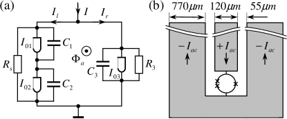
Figure 1: Three-junction SQUID: Equivalent circuit (a) and schematic layout (b).

We first discuss the underlying dynamic equations, using the resistively and capacitively shunted junction modelStewart (1968); McCumber (1968). To simplify the layout, junctions 1,2 in the left arm are shunted by a common resistor $R_{s}$, in contrast to the original proposalZapata et al. (1996), where junctions 1,2 are shunted individually. With Kirchhoff’s laws, the Josephson equations and the phase differences $\delta_{k}$ across junction $k=1,2$, the current $I_{l}$ through the left arm is

$$\frac{I}{2}+J=I_{l}=\frac{\Phi_{0}C_{k}}{2\pi}\ddot{\delta_{k}}+\frac{\Phi_{0}}{2\pi R_{s}}(\dot{\delta_{1}}+\dot{\delta_{2}})+I_{0k}\sin{\delta_{k}}+I_{Ns}.$$ (1a)

$$\Phi_{0}=h/2e I_{Ns} S_{I}(f)=4k_{B}T/R_{s} R_{s} \Phi_{0}(\dot{\delta_{1}}+\dot{\delta_{2}})/2\pi R_{s} \Phi_{0}\dot{\delta_{k}}/2\pi R_{k} I_{r}$$ is the flux quantum; is the Nyquist noise current (with spectral density ) produced by the shunt. We neglect the (subgap) resistances of the unshunted junctions which are much larger than . Note that the original modelZapata et al. (1996) can be obtained from (1a) by replacing by . The current through the right arm is

$$\frac{I}{2}-J=I_{r}=\frac{\Phi_{0}C_{3}}{2\pi}\ddot{\delta_{3}}+\frac{\Phi_{0}}{2\pi R_{3}}\dot{\delta_{3}}+I_{03}\sin{\delta_{3}}+I_{N3}\;.$$ (1b)

The total bias current is $I=I_{l}+I_{r}$, and the Langevin equations(1a), (1b) are coupled via the circulating current around the loop $J=(I_{l}-I_{r})/2$. The phase differences $\delta_{k}$ are connected via

$$\delta_{3}-(\delta_{1}+\delta_{2})=\frac{2\pi}{\Phi_{0}}(\Phi_{a}+LJ)=\frac{2\pi}{\Phi_{0}}\Phi_{T}\;.$$ (2)

The total flux $\Phi_{T}$ through the SQUID loop has contributions from the applied flux $\Phi_{a}$ and from the circulating current $J$. For comparison with experimental results, we performed numerical simulations to solve the coupled Langevin equations (1a), (1b) and (2). From the second Josephson relation we obtain the momentary voltage across the junctions ($U_{k}=\Phi_{0}\dot{\delta_{k}}/2\pi$) and, by time averaging, the dc voltage $V$ across the SQUID and thus the current voltage characteristic (IVC) and the critical current $I_{c}$ vs. applied flux $\Phi_{a}$.

In the following we derive the ratchet potential in the overdamped limit, i.e. with $\beta_{Ck}\equiv 2\pi I_{0k}R_{k}^{2}C_{k}\ll 1$ for all three junctions. The displacement currents $\propto C_{k}\ddot{\delta_{k}}$ in (1a), (1b) can then be neglected and the equations of motion reduce to only two differential equations

$$I_{l} =\frac{\Phi_{0}}{2\pi R_{s}}(\dot{\delta_{1}}+\dot{\delta_{2}})+I_{01}\sin{\delta_{1}}+I_{Ns}\;,$$ (3a)

$$I_{r} =\frac{\Phi_{0}}{2\pi R_{3}}\dot{\delta_{3}}+I_{03}\sin{\delta_{3}}+I_{N3}\;,$$ (3b)

plus conservation of the supercurrent in the left arm $I_{01}\sin{\delta_{1}}=I_{02}\sin{\delta_{2}}$, which can be used to express the overall phase difference for the left arm $\delta_{l}\equiv\delta_{1}+\delta_{2}$ in terms of $\delta_{1}$ only

$$\delta_{l}=\delta_{1}+\arcsin{(q\sin{\delta_{1}})}\;,$$ (4)

with $q\equiv I_{01}/I_{02}$. Without loss of generality we assume $I_{01}\leq I_{02}$, i.e. $q\leq 1$. Equation (4) can be reversed to

$$\delta_{1}=\arctan{\Bigl{(}\frac{\sin{\delta_{l}}}{\cos{\delta_{l}+q}}\Bigr{)}}\;.$$ (5)

Inserting (5) and the expression for the circulating current (2) into (3b) and (3a) leads to

$$\frac{\Phi_{0}}{2\pi R_{3}}\dot{\delta_{3}}-\frac{I}{2}+I_{N3} = -I_{03}\sin{\delta_{3}}-\frac{\Phi_{0}}{2\pi L}(\delta_{3}-\delta_{l}-2\pi\frac{\Phi_{a}}{\Phi_{0}})$$ (6a)

$$\equiv -\frac{\partial U}{\partial\delta_{3}},$$

$$\frac{\Phi_{0}}{2\pi R_{s}}\dot{\delta_{l}}-\frac{I}{2}+I_{Ns} = -I_{01}\sin{(\arctan{\Bigl{(}\frac{\sin{\delta_{l}}}{\cos{\delta_{l}}+q}\Bigr{)}})}$$

$$+\frac{\Phi_{0}}{2\pi L}(\delta_{3}-\delta_{l}-2\pi\frac{\Phi_{a}}{\Phi_{0}})\equiv-\frac{\partial U}{\partial\delta_{l}}\;.$$

The potential $U(\delta_{l},\delta_{3})$ is obtained by integration as

$$U(\delta_{l},\delta_{3}) = -sI_{01}\cos{\delta_{3}}+\frac{\Phi_{0}}{4\pi L}(\delta_{3}-\delta_{l}-2\pi\frac{\Phi_{a}}{\Phi_{0}})^{2}$$ (7)

$$\mp\frac{I_{01}}{q}(\sqrt{1+2q\cos{\delta_{l}}+q^{2}}+q-1)\;.$$

The minus (plus) sign in the second line applies for $\cos(\delta_{l}/2)>0$ ($<0$). The symmetry of $U$ is determined by the applied flux and $s\equiv I_{03}/I_{01}$. If the screening parameter $\beta_{L}\equiv 2LI_{0}/\Phi_{0}\ll 1$ (with $I_{0}\equiv(I_{03}+I_{01})/2$), the phase differences are fixed by the applied flux $\Phi_{a}$ i.e. $\delta_{3}-\delta_{l}=2\pi\Phi_{a}/\Phi_{0}$; hence $\delta_{3}$ can be eliminated:

$$U(\delta_{l}) = -sI_{01}\cos{(\delta_{l}+2\pi\frac{\Phi_{a}}{\Phi_{0}})}$$ (8)

$$\mp\frac{I_{01}}{q}(\sqrt{1+2q\cos{\delta_{l}}+q^{2}}+q-1)\;.$$

If the two junctions in the left arm have equal critical currents ($q=1$) the above expression turns into

$$U(\delta_{l})=-sI_{01}\cos{(\delta_{l}+2\pi\frac{\Phi_{a}}{\Phi_{0}})}-2I_{01}\cos{(\delta_{l}/2)}\;,$$ (9)

which coincides with the result presented inZapata et al. (1996) and is shown in Fig. 2 for $s=1/2$ (the value proposed inZapata et al. (1996)).

Figure 2: Potential $U$ from eq.(9) for $s=1/2$, and two values of applied flux $\Phi_{a}$.

As one can see from Fig. 2, it is the applied flux that breaks the reflection symmetry of the potential. The critical currents $I_{c}^{+}(\Phi_{a})$, $I_{c}^{-}(\Phi_{a})$ represent the force to overcome the potential barrier for positive and negative bias current polarity, respectively. Hence, measuring $I_{c}^{\pm}$ provides a way to probe the asymmetry of the potential. The maximum of $I_{c}(\Phi_{a})=2I_{0}$ is reached if each arm carries a current, that is equal to its critical current, i.e. $I_{r}=I_{03}$ and $I_{l}=I_{01}$. The circulating current is then given by $J=(I_{01}-I_{03})/2$, and the three phase differences have the values $\delta_{1}=\delta_{3}=\pi/2$ and $\delta_{2}=\arcsin q\leq\pi/2$. Inserting this into (2) and solving for $\Phi_{a}$ gives the applied flux $\Phi_{a}^{\pm}$ at maximum $I_{c}$ ($+$ and $-$ corresponds to positive and negative bias current, respectively)

$$\Phi_{a}^{\pm}=\mp\frac{\Phi_{0}}{4}\bigl{(}\frac{2}{\pi}\arcsin q+2\beta_{L}\frac{1-s}{1+s}\bigr{)}\;.$$ (10)

If $q\approx 1$, the first term yields a shift $\approx\mp\Phi_{0}/4$ of the $I_{c}^{\pm}(\Phi_{a})$-dependence. The second term has the same sign and is proportional to $\beta_{L}$. Equation (10) can be used to estimate $q$, $\beta_{L}$ and $s$ from the measured $I_{c}(\Phi_{a}$).

The 3JJ SQUIDs we investigated were fabricated at HYPRES using Nb/Al-AlO_x/Nb  junctions of nominal critical current density $j_{0}=1\,\rm{kA/cm^{2}}$ at $T$=4.2 K, capacitance per area $C^{\prime}=38\,\rm{fF/\mu m^{2}}$ and nominally identical shunt resistors $R_{s}=R_{3}$. Junction areas $A_{J,1}=A_{J,2}=3.8\times 3.8\mu\rm{m}^{2}$, and $A_{J,3}=2.6\times 2.6\mu\rm{m}^{2}$, correspond to $s\approx 1/2$ and $q=1$. For microwave irradiation (up to $28\,\rm{GHz}$), the SQUIDs are integrated in a coplanar waveguide (see Fig. 1(b)) with $50\,\Omega$ impedance. In total we investigated six devices which differed by the size of the SQUID hole, i.e. by the SQUID inductance $L$. All devices showed very similar behavior. Below we discuss only one device with a $2\times 3\mu\rm{m^{2}}$ hole. All measurements were performed at $T=4.2\,K$ in a magnetically and electrically shielded environment, with low pass filters in the voltage leads. Apart from microwave drives we also studied the ratchet behavior in the kHz regime with ac currents directly fed into the bias leads.

Fig. 3(a) shows a measured IVC ($\Phi_{a}=0$) with normal resistance $R_{n}\approx 0.7\,\Omega$, and thus $R_{s}\approx R_{3}\equiv R\approx 1.4\,\Omega$. The inset shows the critical currents $I_{c}^{\pm}(\Phi_{a})$ with maximum $I_{c}=2I_{0}=186\mu\rm{A}$, giving a noise parameter $\Gamma\equiv 2\pi k_{B}T/(I_{0}\Phi_{0})\approx 2\cdot 10^{-3}$, characteristic voltage $V_{c}\equiv I_{0}R=130\,\mu\rm V$ and characteristic frequency $f_{c}\equiv V_{c}/\Phi_{0}=63\,\rm GHz$. With the design values for the junction capacitances $C_{1}=C_{2}=0.54\,$pF and $C_{3}=0.27\,$pF we obtain $\beta_{C,1}=\beta_{C,2}=0.38$ and $\beta_{C,3}=0.09$. The shape (asymmetry) and modulation depth of $I_{c}(\Phi_{a})$ is determined by $s$, $q$ and $\beta_{L}$. Adjusting these parameters in numerical simulations of $I_{c}(\Phi_{a})$ (with values for $\Gamma$ and $\beta_{Ck}$ as determined above), we find best agreement with the measured $I_{c}(\Phi_{a})$ for $\beta_{L}=0.1$, $s=0.5$ and $q=0.99$. These parameters are very close to the design values, and have been used later to numerically calculate the response of the SQUID to an ac bias current.

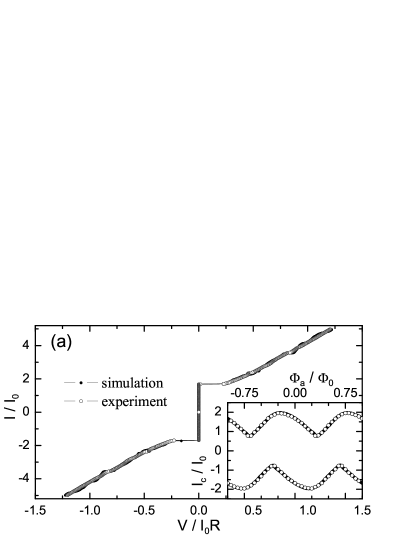
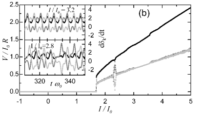
Figure 3: SQUID characteristics without ac drive: (a) $I(V)$-curves ($\Phi_{a}=0$) and $I_{c}(\Phi_{a})$ (inset). (b) Simulated $V(I)$-curve (black) and individual voltages across junction 1 (grey) and 2 (light grey). Insets: Voltage vs. time for junction 3 (black), 1 (grey) and 2 (light grey) for $I/I_{0}=3.2$ and $2.8$. Parameters for numerical simulations: $\Gamma=2\cdot 10^{-3}$, $\beta_{C,1}=\beta_{C,2}=0.38$, $\beta_{C,3}=0.09$, $\beta_{L}=0.1$, $s=0.5$ and $q=0.99$.

As a prominent feature in the experimental zero field IVCs, we observe step-like structures in the resistive state; simulated IVCs exhibit the same generic shape [cf. Fig. 3(a)]. The simulation allows to trace the individual voltage drops across the junctions, as shown in Fig. 3(b). It turns out that the step structures in the IVCs can be associated with switching of junctions 1 and 2 between different states: (i) one junction is in the zero voltage state while the other carries a large voltage; (ii) both junctions are in the voltage state and oscillate coherently, i.e. with the same frequency; typically these oscillations are out of phase [cf. upper inset in Fig. 3(b)]; (iii) both junctions are in the voltage state; however, oscillations are irregular and incoherent [cf. lower inset in Fig. 3(b)]. This state is associated with a more ”noisy” IVC as compared to (ii). Our simulations show that over a wide range of bias currents the junctions oscillate incoherently and thus are far from the scenario discussed inZapata et al. (1996), where junctions 1 and 2 were assumed to behave identical, i.e. $\delta_{1}=\delta_{2}$ at all times (”synchronous state”).

We performed extensive numerical simulations to compare our device (with common shunt for junctions $1,2$) with the one in Zapata et al. (1996). For $T=0$ both devices exhibit phase synchronous oscillations over the entire range of bias currents if junctions 1,2 are identical and with initial values $\delta_{k}=0$ and $\dot{\delta}_{k}=0$. However, choosing either different initial conditions or non-identical junction parameters results in a behavior very similar to the one shown in Fig. 3(b). At $T=0$ the synchronous state is more easily destroyed if junctions 1,2 have a common shunt, as compared to being shunted individually. In the latter case, the synchronous state is more stable, due to a damping term $\propto\partial(\delta_{1}-\delta_{2})/\partial t$ which is absent in the equations of motion for the system with common shunt for junctions 1,2Sterck et al. (2005). However, thermal fluctuations at finite temperature, also tend to destroy the synchronous state for the individually shunted 3JJ SQUID. Hence, for the experimentally relevant case, i.e. at finite temperature ($\Gamma{\scriptscriptstyle\stackrel{{\scriptstyle>}}{{\sim}}}10^{-3}$) and slight junction asymmetries ($q\neq 0$), both types of SQUID ratchets show typically incoherent oscillations of junctions 1,2.

Figure 4: Rectified voltage vs. ac drive amplitude at $\Phi_{a}=\Phi_{0}/4$ for a 3JJ SQUID ratchet with increasing drive frequency $f$ (from top to bottom). Left column shows experimental data at $T=4.2\,\rm{K}$ (insets in (c),(e) show enlarged section of one voltage step) and right column shows the corresponding simulated curves (parameters as in Fig. 3). The dashed lines in (b), (d), (f) were calculated for $T=0$, with $I_{01}=I_{02}$ ($q=1$) and $\delta_{k}=\dot{\delta}_{k}=0$ ($k=1,2$) at $t=0$ .

Fig. 4 shows experimental data, and numerical simulation results, for the rectified voltage $V$ under ac drive $I=I_{ac}\sin 2\pi ft$, clearly demonstrating operation of the SQUID as a rocking ratchet. For adiabatic drive $f\ll f_{c}$ [c.f. Fig. 4(a)] rectification appears at $I_{ac}{\scriptscriptstyle\stackrel{{\scriptstyle>}}{{\sim}}}I_{0}$. $V$ sharply peaks at $I_{ac}\approx 2I_{0}$ and decreases again with increasing $I_{ac}$, as predicted for a 1D rocking ratchetBartussek et al. (1994) and as observed experimentally for asymmetric (two junction) dc SQUID ratchetsWeiss et al. (2000); Sterck et al. (2002). In contrast to the prediction for overdamped rocking ratchets Bartussek et al. (1994); Borromeo et al. (2002), the initial increase in $V(I_{ac})$ up to the maximum $V_{max}$ is not linear. Instead, it sets off with a very steep slope $dV/dI_{ac}$ which becomes smaller at higher voltage. A strikingly similar behavior has been predicted for a strongly underdamped rocking ratchet Borromeo et al. (2002). In our case, the motion of $\delta_{l}$ is overdamped; however for $\delta_{1}-\delta_{2}$ it is underdamped, which obviously gives the same result as reported in Borromeo et al. (2002). $V_{\rm max}=25\mu\rm{V}$ is as large as 20% of $V_{c}$, in excellent agreement with simulations shown in Fig. 4(b). As maximum rectification requires $\Phi_{a}^{+}-\Phi_{a}^{-}\approx\Phi_{0}/2$, it is easy to understand from eq.(10) why the 3JJ SQUID ratchet is superior to the asymmetric dc SQUID ratchet: For the asymmetric dc SQUID the arcsin-term in (10) is absent, and the shift in the $I_{c}^{\pm}(\Phi_{a})$-curves is determined by $\beta_{L}$ and $s$ only. Hence, the condition for maximum rectification depends strongly on the SQUID parameters and is more difficult to fulfill experimentally. In contrast, for the 3JJ SQUID, it is sufficient to keep $\beta_{L}$ small, so that the arcsin-term dominates. For $q\approx 1$, the condition for maximum rectification is then easy to achieve experimentally.

At nonadiabatic drive frequencies [c.f. Fig. 4(c),(e)] we observe a step-like increase of $V(I_{ac})$ up to $V_{max}$ and oscillations in $V(I_{ac})$ for higher drive amplitudes. The voltage steps appear at $V/(I_{0}R)=n\cdot(f/f_{c})$ ($n$: integer) and can be interpreted as Shapiro steps, where the phase dynamics synchronizes with the external driveSterck et al. (2002). This quantization of the ratchet effect has been predicted as a characteristic feature of nonadiabatically driven 1D rocking ratchets Bartussek et al. (1994); Zapata et al. (1996); however, it has not been observed experimentally until now, due to thermal noise smearingSterck et al. (2002). For the same reason, $V(I_{ac})$ oscillates at higher drive amplitudes, rather than showing a step-like behavior. This effect of thermal noise was also predicted inBartussek et al. (1994) for 1D rocking ratchets and is clearly demonstrated for our device in the simulations of $V(I_{ac})$ shown in Fig. 4(d), (f) for finite and zero $T$. For finite $T$, our simulations nicely reproduce the experimental data. For the case $T=0$, simulations were performed with $q=1$ and identical initial conditions $\delta_{1,2}=\dot{\delta}_{1,2}=0$. This leads to the formation of the synchronous state (i.e. $\delta_{1}=\delta_{2}$ at all times). Only in this case a step-like switching of the rectification is observed in the numerical simulations also at large ac drive amplitudes; i.e. experimental observation of quantized rectification for large driving amplitudes, will be quite difficult. Furthermore, we note that only in the synchronous state ($\varphi\equiv\delta_{1}-\delta_{2}=0$) the dynamics of the system is described by $\delta_{l}(t)$ only, as the motion of a particle in the 1-dimensional potential (9) which is $4\pi$-periodic in $\delta_{l}$. In contrast, if $\dot{\varphi}\neq 0$, the dynamics can be described in a 2-dimensional potential along $\delta_{l}$ and $\varphi$ Sterck et al. (2005). This potential has minima which are separated by $2\pi$ if projected onto the $\delta_{l}$-axis. This explains the doubling of the Shapiro step height calculated for the synchronous state [c.f. dashed lines in Figs. 4(d),(f)] as compared to the calculations for finite $T$ and as observed experimentally [c.f. Figs.4(c),(e)].

In conclusion, following a proposal inZapata et al. (1996), we have realized 3JJ SQUIDs and demonstrated operation of those devices as very efficient rocking ratchets. In contrast to the original proposal, which assumed that the two junctions connected in series oscillate in-phase, we found that these junctions usually oscillate incoherently. Nonetheless the devices show a large ratchet effect, more than two orders of magnitude above initial estimates given inZapata et al. (1996). Apart from rectification of a harmonic low-frequency drive, we find rectification of nonadiabatic drives with striking properties, such as Shapiro-like steps, i.e. quantization of the velocity of directed motion, which depends only on the drive frequency. The simplicity of the design, the good experimental control over external drives and device parameters which define e.g. the shape of the ratchet potential, and, finally, easy detection of directed motion by measuring voltage, gives this device excellent perspectives for further basic experimental studies of ratchet effects, e.g. for stochastic drives.

We gratefully acknowledge financial support from the Deutsche Forschungsgemeinschaft.

References

- Reimann (2002) P. Reimann, Physics Reports 361, 57 (2002).
- Linke (2002) H. Linke, Appl. Phys. A 75, 167 (2002), guest editor.
- Magnasco (1993) M. O. Magnasco, Phys. Rev. Lett. 71, 1477 (1993).
- Bartussek et al. (1994) R. Bartussek, P. Hänggi, and J. G. Kissner, Europhys. Lett. 28, 459 (1994).
- Faucheux et al. (1995) L. P. Faucheux, L. S. Bourdieu, P. D. Kaplan, and A. J. Libchaber, Phys. Rev. Lett. 74, 1504 (1995).
- Mateos (2000) J. L. Mateos, Phys. Rev. Lett. 84, 258 (2000).
- Borromeo et al. (2002) M. Borromeo, G. Costantini, and F. Marchesoni, Phys. Rev. E 65, 041110 (2002).
- Wambaugh et al. (1999) J. F. Wambaugh, C. Reichhardt, C. J. Olson, F. Marchesoni, and F. Nori, Phys. Rev. Lett. 83, 5106 (1999).
- Lee et al. (1999) C.-S. Lee, B. Jankó, I. Derény, and A.-L. Barabási, Nature 400, 337 (1999).
- Olson et al. (2001) C. J. Olson, C. Reichhardt, B. Janko, and F. Nori, Phys. Rev. Lett 87, 177002 (2001).
- Villegas et al. (2003) J. E. Villegas, S. Savel’ev, F. Nori, E. M. Gonzalez, J. V. Anguita, R. Arcía, and J. L. Vicent, Science 302, 1188 (2003).
- Van de Vondel et al. (2005) J. Van de Vondel, C. C. de Souza Silva, B. Y. Zhu, M. Morelle, and V. V. Moshchalkov, Phys. Rev. Lett. 94, 057003 (2005).
- Trías et al. (2000) E. Trías, J. J. Mazo, F. Falo, and T. P. Orlando, Phys. Rev. E 61, 2257 (2000).
- Goldobin et al. (2001) E. Goldobin, A. Sterck, and D. Koelle, Phys. Rev. E 63, 031111 (2001).
- Carapella and Costabile (2001) G. Carapella and G. Costabile, Phys. Rev. Lett. 87, 077002 (2001).
- Carapella et al. (2002) G. Carapella, G. Costabile, N. Martucciello, M. Cirillo, R. Latempa, A. Polcari, and G. Filatrella, Physica C 382, 337 (2002).
- Beck et al. (2005) M. Beck, E. Goldobin, M. Neuhaus, M. Siegel, R. Kleiner, and D. Koelle, Phys. Rev. Lett. (to be published).
- Zapata et al. (1996) I. Zapata, R. Bartussek, F. Sols, and P.Hänggi, Phys. Rev. Lett. 77, 2292 (1996).
- Weiss et al. (2000) S. Weiss, D. Koelle, J. Müller, R. Gross, and K. Barthel, Europhys. Lett. 51, 499 (2000).
- Sterck et al. (2002) A. Sterck, S. Weiss, and D. Koelle, Appl. Phys. A 75, 253 (2002).
- Berger (2004) J. Berger, Phys. Rev. B 70, 024524 (2004).
- Stewart (1968) W. C. Stewart, Appl. Phys. Lett 12, 277 (1968).
- McCumber (1968) D. McCumber, J. Appl. Phys. 39, 3113 (1968).
- Sterck et al. (2005) A. Sterck, R. Kleiner, and D. Koelle, unpublished (2005).