Itinerancy and Hidden Order in
Abstract
We argue that key characteristics of the enigmatic transition at in indicate that the hidden order is a density wave formed within a band of composite quasiparticles, whose detailed structure is determined by local physics. We expand on our proposal (with J.A. Mydosh) of the hidden order as incommensurate orbital antiferromagnetism and present experimental predictions to test our ideas. We then turn towards a microscopic description of orbital antiferromagnetism, exploring possible particle-hole pairings within the context of a simple one-band model. We end with a discussion of recent high-field and thermal transport experiment, and discuss their implications for the nature of the hidden order.
I Introduction
The possibility of exotic particle-hole pairing leading to quadrupolar and orbital charge currents has been discussed extensively in the context of the two-dimensional Hubbard model.Halperin68 ; Affleck88 ; Kotliar88 ; Nersesyan89 ; Schulz89 More recently d-wave charge-density wave states, both orderedChakravarty01 and fluctuating,Lee04 have been proposed to explain the pseudogap phase in the underdoped cuprates and ground-states of doped two-leg Hubbard and ladders.Fjaerestad02 ; Wu04 In this paper we discuss related anisotropic particle-hole pairing in a different setting, namely that of three-dimensional Fermi liquids. We believe that such pairing may occur in the heavy fermion metal , and here we provide theoretical support for our earlier publications (with J.A. Mydosh) on this topic.Chandra02a ; Chandra02b ; Mydosh03 ; Chandra03 Though the initial motivation for our orbital antiferromagnetism (OAFM) proposal in was primarily experimental, here we observe that coexistence of large electron-electron repulsion and antiferromagnetic fluctuations favours node formation in particle-hole pairing and hence the formation of anisotropic charge-density wave states. After presenting technical details behind specific predictions for neutron scattering and for NMR, we turn towards a microscopic description of orbital antiferromagnetism. We start by presenting the generalised Landau parameters associated with this anisotropic pairing. Next we study a toy model where this instability occurs. We end with a discussion of these results in the light of more recent measurements, and also suggest further experiments to test our ideas.
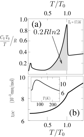 |
The heavy fermion metal displays a classic second-order phase transition (see Figure 1) at , and yet the nature of the associated order parameter remains elusive nearly two decades after its discovery. This phase transition is characterised by a large entropy lossPalstra85 and sharp anomalies in the linearPalstra85 and the nonlinear susceptibilities,Miyako91 ; Ramirez92 the thermal expansion,deVisser86 and the resistivity,Palstra86 where standard mean-field relations between measured thermodynamic quantities are satisfied.Chandra94 At the transition, neutron scattering experiments observe gapped, propagating magnetic excitationsWalter86 ; Mason91 ; Broholm87 ; Broholm91 that suggest the formation of a spin density wave. However, subsequent neutron scattering measurementsBroholm87 ; Broholm91 indicate that the staggered magnetic moment ( per U atom), is too small to account for the entropy loss at the transition,Buyers96 which has been attributed to the development of an enigmatic hidden order.
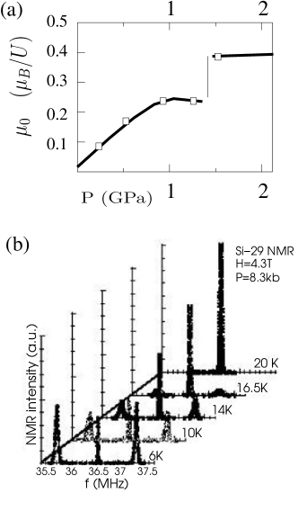
There is strong experimental evidence that the antiferromagnetism and the hidden order in are phase-separated and thus develop independently.Chandra03 High-field measurementsMentink96 ; vanDijk97 ; Bourdarot03 indicate that the bulk anomalies survive up to 40 Tesla (), while the staggered moment is destroyedMason95 by comparatively modest fields of 15 . Furthermore, the staggered magnetic moment grows linearly with pressureAmitsuka99 while bulk anomalies associated with the hidden order remain relatively pressure-independent.Fisher90 Phase separation is also indicated by muon spin resonance experiments.Luke94 ; Amitsuka03 The most direct evidence has come from recent NMR pressure-dependent measurements (see Figure 2):Matsuda01 for the existence of distinct antiferromagnetic and paramagnetic (hidden order) phases is clearly observed in samples with less than of the volume magnetic () at ambient pressure. The observed increase of the staggered magnetic moment with pressureAmitsuka99 is then simply a volume-fraction effect.Matsuda01 The magnetic order develops independently from the hidden order through a first order transition,Chandra02a and the associated temperature-pressure phase diagram has been determined using thermal expansion measurements.Motoyama02
The mysterious phase transition at has features that have both local and itinerant electronic natures, and these coexisting dual characteristics make its description quite challenging. For example, the development of a sharp propagating mode just below observed by inelastic neutron scattering Walter86 ; Broholm87 ; Mason91 emphasises the importance of local crystal-field excitations at the transition. Nevertheless a purely local picture cannot provide a straightforward explanation for the observed elastic anomaliesLuthi93 near that are distinct from those of typical uniaxial antiferromagnetsMelcher70 both due to their (weak) magnitudes and due to the absence of precursor effects for .
 |
The sharp mean-field nature of the phase transition at , together with the magnitude of the condensation entropy and the observed development of gap in the excitation spectrum all suggest the development of density-wave order within a fluid of itinerant quasiparticles.Ramirez92 ; Chandra94 ; Chandra02b ; Virosztek02 Itineracy is implicated by the sharpness of the transition while gap formation and the large entropy of condensation speak in favour of an order parameter at a finite wavevector. However, a dissenting view on this last point, involving p-wave ferromagnetism, has recently been proposed.Varma05 We note that within the itinerant perspective presented here, there are problems matching details of the excitation spectra as observed in inelastic neutron scattering experiments.Broholm91 On the other hand, a purely local scenarioBroholm91 ; Santini94 (with anticipated corrections for itinerant fermions) simply can not be reconciled with the almost complete quenching of the local moments, implicated by the paramagnetic (as opposed to Curie-like) susceptibility (see inset Fig. 1b.) and the large linear specific capacity, normally associated with well-formed heavy electrons (Fig. 1a). There are addition inconsistencies with a local picture: for example, the gap used in the local singlet schemeBroholm91 to explain the dispersing magnetic mode has a different field-dependence from that of the bulk associated with thermodynamic quantities.Santini00 A strict adherence to a local scheme requires consideration of many additional crystal-field levelsSantini00 evolving differently in an applied field.
A proper theoretical description of the transition at in must therefore encompass both local and itinerant features of the problem. More specifically, the observed Fermi liquid properties for (e.g. Fig. 1) combined with the large entropy loss and the sharp nature of the transition indicate that the underlying quasiparticle excitations are itinerant, presumably composite objects formed from the 5f spin and orbital degrees of freedom of the ions. Local physics (e.g. Kondo physics, spin-orbit coupling, crystal-field schemes) plays a key role in their development.
We have just outlined a number of general considerations that we believe are crucial features of the hidden order in . Given these criteria, we (with J.A. Mydosh) have proposed that it can be described by a general density wave whose form factor is constrained by experimental observation and is ultimately determined by underlying local excitations.Mydosh03 We note that a number of proposals for the hidden order that fit into this general framework have been made.Chandra94 ; Virosztek02 ; Amitsuka02 ; Kiss04 ; Mineev04 ; Varma05 We argue that the large entropy loss at the transition can only be understood if the density-wave involves the polarisation of a significant fraction of the quasiparticle band, a condition that discounts a conventional spin-density wave due to the small size of the observed magnetic moment. Taking our cue from ambient-pressure Si NMR measurements (see Figure 3) that indicate broken time-reversal symmetry in the hidden ordered phase,Bernal01 we (with J.A. Mydosh) have proposed that becomes an incommensurate orbital antiferromagnet at with charge currents circulating between the uranium ions.Chandra02b Here the modulation wavevector is chosen to fit the observed isotropic field distribution at the silicon sites. The resulting real-space fields can then be Fourier transformed to calculate a neutron scattering structure factor with a ring of possible q-vectors. Though these results have been presented elsewhere,Chandra02b in this paper (Section II) we provide supporting technical details and further discussion. We also determine the NMR linewidths at the Ru sites. Detailed comparison with recent experiment puts constraints on the allowed incommensurate wavevectors, allowing us to make more specific predictions for neutron scattering measurements.
In the second part of this paper, we turn towards an underlying microscopic picture of orbital antiferromagnetism. More specifically, in Section III we explore particle-hole pairings in anisotropic incompressible Fermi liquids with specific application to Next (Section IV) we introduce a simple model with a single heavy band and weak antiferromagnetic spin fluctuations (AFMSF). We note that this particular Hamiltonian was originally introducedMiyake86 to describe the AFMSF-mediated transition in at . We show that this same toy model also supports particle-hole pairings associated with incommensurate orbital antiferromagnetism and quadrupolar charge-density wave formation. We end (Section IV) the paper with a summary, and then discuss our results in the context of recent high-field and thermal transport measurements.
II Phenomenology and Experimental Predictions
In this Section we review the experimental motivation for incommensurate orbital antiferromagnetism as the hidden order in . We develop the phenomenology of this proposal, independent of microscopic details. The magnitude and the ordering wavevector of the orbital currents are fittedChandra02b to the observed isotropic field-distribution at the silicon sites as measured by nuclear magnetic resonance (NMR).Bernal01 The real-space fields produced by the orbital charge currents at all points in the sample volume are then determined, and we use this information to make specific predictions for neutron scattering structure factors and for NMR at non-silicon sites to test this proposal.
II.1 Incommensurate Orbital Antiferromagnetism as the Hidden Order in
We begin our phenomenological discussion by reviewing the case for incommensurate orbital antiferromagnetism as the hidden order in . There have been many proposals for the primary order parameter in this material,Virosztek02 ; Amitsuka02 ; Kiss04 ; Mineev04 ; Varma05 ; Shah00 and until recently it was assumed that the spin antiferromagnetism and the hidden order are coupled and homogenous. However pressure-dependent NMR measurements,Matsuda01 supported by muon spin resonanceLuke94 ; Amitsuka03 and thermal expansionMotoyama02 data, indicate that the hidden and the magnetic orders are phase-separated and thus are completely independent.Chandra03
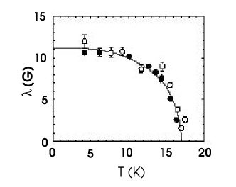 |
We believe that an important clue to the nature of the hidden order in is provided by Si NMR measurements at ambient pressureBernal01 that indicate that at the paramagnetic (non-split) silicon NMR line-width develops a field-independent, isotropic component whose temperature-dependent magnitude is proportional to that of the hidden order parameter. These results imply an isotropic field distribution at the silicon sites whose root-mean square value is proportional to the hidden order ()
| (1) |
and is Gauss at . This field magnitude is too small to be explained by the observed momentBroholm87 that induces a field Gauss where is the bond length ( cm). Furthermore this moment is aligned along the -axis, and thus cannot account for the isotropic nature of the local field distribution detected by NMR. These measurements indicate that as the hidden order develops, a static isotropic magnetic field develops at each silicon site. This is strong evidence that the hidden order parameter breaks time-reversal invariance.
The magnetic fields at the silicon nuclei have two possible origins:Schlichter78 the conduction electron-spin interaction and the orbital shift that is due to current densities. In , the observed Knight shiftBernal01 indicates a strong Ising anisotropy of the conduction electron fluid along the axis; therefore the electron-spin coupling is unlikely to be responsible for the measured isotropic field distribution at the Si sites. It thus seems natural that these local fields are produced by orbital currents that develop at , and thus we attribute the observed isotropic linewidth to the orbital shift.
It is this line of reasoning that led us (with J.A. Mydosh) to proposeChandra02b that is an incommensurate orbital antiferromagnet at with charge currents circulating between the uranium ions. The planar tetragonal structure of presents a natural setting for an anisotropic charge instability of this type. We can estimate the local fields at the silicon sites that are produced by the orbital currents. On dimensional grounds, the current along the uranium-uranium bond is given by where is the gap associated with the formation of the hidden order at ; we note that this expression also emerges from an analysis of the Hubbard model.Affleck88 If this orbital charge current is flowing around a uranium plaquette of side length , then the magnetic field produced at a height above it is given by Ampere’s Law to be , in good agreement with the observed field strength;Bernal01 here we have used the experimental valuePalstra85 . Note that the resulting orbital moment, (), is comparable to the effective spin moment at ambient pressure. We emphasise that an orbital moment produces a field an order of magnitude less than that associated with a spin moment of the same value; the low field strengths observed at the silicon sites are quantitatively consistent with our proposal that they originate from charge currents.
This orbital moment, , can also account for the entropy loss at the transition. We emphasise that its large value suggests that the amplitude of any proposed density-wave must be a significant fraction of its maximally allowed value, and will proceed to show that this is the case for the OAFM. In a metal the change in the entropy is given by where is the change in the linear specific heat coefficient resulting from the gapping of the Fermi surface. is inversely proportional to the Fermi energy of the gapped Fermi surface, so that in general the change in entropy per unit cell is given by . Since the transition at is mean-field in nature,Chandra94 we have so that . Now we recall that the orbital magnetic moment is
| (2) |
such that it is saturated when
| (3) |
analogous to the saturation value of the electron spin where and are the Bohr radius and the energy of the Hydrogen atom respectively; here we have used and where and refer to the mass of hydrogen and of respectively. Then the change in entropy at the transition () due to the development of orbital antiferromagnetism can be expressed as
| (4) |
which is a number () in good agreement with experiment.Palstra85 We also note that the critical field for suppressing the thermodynamic anomalies is distinct from its spin counterpart: the ratio is qualitatively consistent with the observed critical field associated with the destruction of hidden order.Mentink96 ; vanDijk97 We emphasise that the sizable entropy loss associated with the development of orbital antiferromagnetism in is a direct consequence of its renormalised electron mass (). More generally the orbital moment is a larger fraction of its saturation value than is its spin counterpart, and this leads to the large entropy loss.
Orbital antiferromagnetism can therefore account for the local field magnitudes at the silicon ions and for the large entropy loss at the transition. Our next step is to tune the ordering wavevector to fit the isotropic distribution at these sites and then to determine the real-space fields throughout the sample volume. This can then be Fourier transformed to make predictions for neutron scattering.Chandra02b We note that it has been suggestedVarma05 that the isotropic nature of the field distributions at the silicon sites may be due to impurity-broadening. Though disorder is certainly present in these samples, we believe that the incommensurate nature of the density wave is the origin of this isotropy. Towards proving this point, we have determined the anisotropic field distributions at non-silicon sites; their observation via NMR would certainly not be possible if there were significant disorder-smearing.
Before proceeding with this program, let us comment briefly on the current experimental situation regarding the proposal of incommensurate orbital antiferromagnetism in . We admit that our proposal is closely linked to the ambient-pressure NMR experiments,Bernal01 which are the only direct evidence of broken time-reversal symmetry in the hidden ordered phase and have not been reproduced by other groups. We note that muon spin resonance measurementsLuke94 ; Amitsuka03 support the emergence of local fields with the same temperature-dependence as that associated with NMR, but their overall amplitudes are two orders of magnitude less than that seen in the NMR measurements. This is a point to which we return in the discussion. Although incommensurate peaks have been seen in inelastic neutron scattering measurements,Broholm91 ; Bull02 ; Wiebe04 , these are due to excitations above the partly gapped Fermi surface and are not directly related to the orbital antiferromagnetism. Current experimental resolution for elastic scattering - a direct probe of the incommensurate orbital antiferromagnetic order - is not yet good enough to confirm or deny the OAFM scenario. Here we present technical support for previous predictions for neutron structure factors,Chandra02b while also making specific suggestions for measurements where the signal should be sufficiently strong to be observed practically.
II.2 Predictions for Neutron Scattering
In order to calculate the neutron cross section for scattering by incommensurate orbital antiferromagnetic order, we use the Born scattering formula,
| (5) |
where is the neutron gyromagnetic ratio, the scattering wavevector of the neutrons, is the structure factor of the magnetic fields produced by the orbital currents and is the structure factor measured in units of the Bohr magneton .
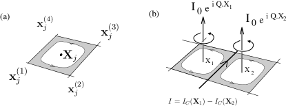
We shall compute the magnetic field as the curl of the vector potential, . The procedure will be to compute the vector potential produced by the circulating current around a given plaquette. We shall denote the co-ordinate of the centre of plaquette j by . The corners of this plaquette are located at sites , () where
as shown in Fig. 4 (a). The circulating current around plaquette is then taken to be
| (6) |
Using Ampere’s law, link 1-2 will will produce a contribution to the vector potential given by
| (7) |
where is the unit vector pointing along the bond from to . Writing as
where defines the position along the link, we have
| (8) |
for the vector potential where is the U-U bond length in the plane.
 |
We now compute , and take the Fourier transform to obtain
| (9) | |||||
Using
we obtain
| (10) | |||||
| (11) |
where we have replaced and
| (12) |
is the form-factor associated with link in the plaquette centred about . To sum over all of the links around the plaquette, we must add together the form factors
| (14) |
We let be the wavevector for the orbital order so that .
Replacing in Eq. 11, we we obtain the complete Fourier transform of the magnetic field:
| (15) |
The U sites can be written as
| (16) |
where is the separation between even or odd numbered U planes. The unit cell has lattice vectors . For an isotropic distribution of magnetic fields at the Si sites, we can reasonably expect to be staggered between successive U layers. We permit to be incommensurate in the plane:
| (17) |
Summing over the lattice sites in Eq.(15) we find
| (18) | |||||
where is a reciprocal lattice vector.
Equation (18) should be contrasted with the corresponding expression if the order parameter were a spin density wave instead of an orbital antiferromagnet:
| (19) | |||||
We note that a major difference between the two cases is that decreases rapidly as while is constant. This makes OAFM much harder to detect in neutron scattering experiments than its SDW counterpart. Second, the term in indicates that scattering is suppressed for since for an SDW along the axis, . here is no such term in . Thus the presence of a finite scattering amplitude at this particular wavevector in would be a “smoking gun” confirmation of incommensurate orbital antiferromagnetism as the hidden order.
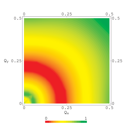
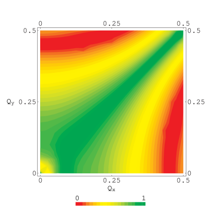
Next we turn to obtaining the structure factor . Neutrons couple to the orbital currents via their magnetic moment () as . For incoherent neutrons, is the modulus squared of averaged over the orientation. the neutrons. Thus
| (20) | |||||
where and is the number of U sites. From this expression, we find that the maximum scattering intensity is predictedChandra02b to lie in a ring of radius centred on the wavevector where lies in the plane. Once again, we emphasise that scattering in the vicinity of is forbidden for the case of ordered spins along the -axis; thus the observed presence of neutron scattering intensity at this particular wavevector would be a “smoking gun” confirmation of orbital antiferromagnetism as the hidden order.
In general the structure factor can be written as a product
| (21) |
where is a function periodic in the reciprocal lattice vector but is not. For the case of orbital antiferromagnetism, the calculated structure factor yields an asymptotic form for the form factor . This power-law decay of the intensity peaks is due to the extended nature of the scattering source in contrast to the exponentially decaying structures observed for point-like spin antiferromagnetism.
It is tempting to state that such power-law peaks will be a clear signature of orbiting charge currents, but we still need to determine whether the overall intensities are observable. We can estimate the strength of the predicted OAFM neutron signal compared to that associated with spin magnetism at ambient pressure. Our calculations indicate that a fifth of the total integrated weight of (TIWSQ) resides in the first Brillouin zone for the OAFM. Using the sum rule that relates the total ISWQ (integrated weight of to the square of the moment, we have
| (22) | |||||
| (23) |
where we have used and . Since the magnetic region occupies roughly a tenth of the sample at ambient pressure we then write
| (24) |
which indicates that the scattering peaks in the first Brillouin zone due to orbital ordering should have roughly 1/50 the intensity of the analogous spin peaks at ambient pressure. There have been two exploratory neutron studiesBull02 ; Wiebe04 but neither was conclusive due to issues of resolution. In particular the more recent elastic measurementsWiebe04 were not performed at the predicted wavevector where there should be no dipole scattering; please recall that here the form factor ) and is aligned with the c-axis. More specifically the scattering intensity should be a factor of twenty higher than at where the experiments were performed, and the experimental resolution should be good enough then to prove/refute the orbital antiferromagnetism proposal.
II.3 Nuclear Magnetic Resonance Linewidth at the Si and the Ru Sites
Nuclear Magnetic Resonance (NMR) is a local probe of the strength and the local distribution of the magnetic field distribution in the material. We use experimental NMR results to determine the ordering wavevector associated with the orbital antiferromagnetism, which can then be included in the structure factor calculated above. Thus neutron scattering and NMR are complementary. Eq.(8) gives the vector potential at a point due to a current in link of a plaquette centred at . Contributions from other links in the plaquette may be similarly written out (see Fig.4). The magnetic field at any point can be obtained using , where is the total vector potential obtained by summing contributions from all links and plaquettes. We give detailed expressions for in the appendix.
For the sake of completeness, we reviewChandra02a ; Chandra02b our arguments regarding the Si NMR measurementsBernal01 and the ordering wavevector of the orbital antiferromagnetism. We note that the silicon atoms in are located at low-symmetry sites above and below the uranium plaquettes, so that the fields there do not cancel. Therefore the proposed OAFM must have an incommensurate in order to produce isotropic field distributions at the silicon sites. If the order parameter in the hidden order phase is OAFM, then such a magnetic field distribution at the Si sites would be possible if the wavevector for orbital ordering were incommensurate,Chandra02a ; Chandra02b
| (25) |
Fig.(5) shows the distribution of the magnetic field lines about the plane for an incommensurate corresponding to in Eq.(25), and viewed in the [010] direction.
A convenient definition of the anisotropy in the magnetic field at a given site is
Fig.(6) shows the anisotropy as a function of the vector. While the field distribution at the Si sites is isotropic, that need not be the case at other sites such as Ru; furthermore the anisotropic nature of the field distribution at the Ru sites would indicate that disorder-averaging is not at play here. If we take as the origin any uranium atom in the lattice, we find the Ru sites at coordinates
| (26) |
where are integers. Fig.7 shows the anisotropy of the magnetic field distribution at the Ru sites.
 |
 |
Recent Ru NMR measurementsBernal04 report a local magnetic field anisotropy of around 0.3. Values of deduced from our OAFM model using the Ru NMR data should of course be consistent with Si NMR. The anisotropy of the magnetic field at the Ru sites calculated from our model shows strong variations as the orientation of the incommensurate wavevector given in Eq.(25) is varied. Anisotropy of field at the Ru sites for OAFM ordering wavevectors given by Eq.(25) varies from about 0.7 along the directions to nearly unity along . Thus the most likely incommensurate wavevector for OAFM lies close to the directions.
Neutron scattering measurementsWiebe04 show enhanced scattering for at the incommensurate wavevectors
| (27) |
where is an odd integer. Below , the ring of excitations seems to collapse toward the and directions, decreasing in intensity. The structure-factor predicted in Eq.(20) could not be verified/refuted due to issues of resolution.Wiebe04 According to Eq.(20), the structure factor measured near , as was done in the most recent experimentWiebe04 has a scattering intensity that is smaller than that at by a factor of more than five. In an earlier experiment,Broholm91 enhanced scattering was observed at above the transition temperature . The scattering intensity was sharply enhanced for , and furthermore, the scattering linewidth decreased to resolution-limited values. More work is needed to verify whether the incommensurate peak observed in neutron scattering measurements is related to Eq.(25) deduced from Si and Ru NMR data using our model of orbital antiferromagnetism, and we strongly suggest elastic neutron scattering measurements at the wavevector predicted to have the greatest intensity () to test OAFM as hidden order.
| Name | T-invariance | Local Fields | |
|---|---|---|---|
| SDW (isotropic spin density wave) | no | yes | |
| CDW (isotropic charge density wave) | const. | yes | no |
| d-SDW | no | no | |
| q-CDW (quadrupolar) | yes | no | |
| OAFM (orbital antiferromagnet) | no | yes |
III Towards a Microscopic Description of the Hidden Order
We now turn to a more microscopic approach to the hidden order. As we have already noted, a proper theoretical description of must encompass both local and itinerant features of the problem. A general duality scheme for heavy electron systems has been proposed.Kuramoto90 In this model, the itinerant excitations are constructed from the low-lying crystal-field multiplets of the uranium atom. The quasiparticles associated with the heavy Fermi liquid are composite objects formed from the localised orbital and spin degrees of freedom of the U ions and the conduction electron fields. The phase transition in this model is then a Fermi-surface instability of these composite itinerant f-electrons. This approach has been adaptedOkuno98 to describe the coexistence of hidden order with a small moment in . With the more recent understanding that the hidden ordered phase does not contain a staggered magnetisation, we have revisited this duality schemeMydosh03 and, guided by experiment, now discuss its implications for the nature of the mysterious order that develops at .
III.1 Possible symmetries for particle-hole pairing
We begin with the assumption that all the excitations of that condense into the hidden ordered state are of itinerant character. More specifically, we will assume that all of the system’s local physics (e.g. local moment character of the f-electrons) has been absorbed into the formation of composite quasiparticles. Given this premise, it then follows that key aspects of the (hidden) order parameter will be expressed through its matrix elements between quasiparticle states. If we denote it by the operator , then its general matrix element between quasiparticle states is
| (28) |
where is the ordering wave-vector and is the quasiparticle state of momentum . Microscopically we would have to characterise in terms of the detailed crystal-field split states of the U ion, but for the purposes of characterising the phase transition, quasiparticle matrix elements should suffice. Within the Hilbert space of the mobile f-electrons, the order parameter can then be written
| (29) |
where is a general function of spin and momentum.
We are therefore considering a class of density waves with the most general pairing in the particle-hole channel characterised by . We now categorise the possible particle-hole pairingsMydosh03 in . Assuming that the hidden order develops between the uranium atoms in each basal plane, we restrict our attention to nearest-neighbour pairings on a two-dimensional square lattice, and display the five resulting possibilities in Table 1 in Eq.(29). We emphasise that each of these pairing choices will partially gap the Fermi surface, accounting for the large entropy loss and the observed anomalies in several bulk quantities.Chandra02b In conventional charge- and spin-density waves (CDWs and SDWs respectively), the quantity is an isotropic function of momentum. However in more general cases will develop a nodal structure which leads to anisotropy (Table 1) that is favoured by strong Coulomb interaction, as we shall discuss in the next section.
III.2 General Discussion of Anisotropic Charge Instabilities in Fermi Liquids
At low temperatures, heavy electron materials form almost incompressible Landau Fermi liquids in which the residual interactions between heavy quasiparticles are driven by strong, low-lying antiferromagnetic spin fluctuations. This harshly renormalised electronic environment is conducive to the development of instabilities in which electrons or holes form bound-states that contain nodes in their pair wavefunction.
Such arguments are well established in the context of anisotropic Cooper pairing.Miyake86 ; Emery87 Here we extend these ideas, arguing that an almost incompressible Fermi liquid is highly susceptible to the formation of anisotropic density waves, where the staggered electron-hole condensate contains a node in the pair wavefunction. This issue first arose in the context of orbital ordering in cuprate superconductorsNayak00 . Here it has been emphasised that strong Coulomb interactions suppress electron-hole bound-state formation in CDWs, unless the bound-state contains a node.Chakravarty01 Heavy electron fluids provide a unique opportunity to apply these arguments to three-dimensional systems. Furthermore there is no controversy associated with the Landau-Fermi liquid of their normal states, a situation in distinct contrast to the situation in the cuprates.
In a heavy electron fluid, the density of states is severely renormalised so that the ratio of the quasiparticle and the bare band-structure density of states
is typically at least a factor of ten. In these systems the magnetic susceptibility, given in Landau Fermi liquid theory by
is weakly enhanced. By contrast, the charge susceptibility is severely depressed by strong coulomb interactions and is essentially given by the unrenormalised band-structure value
which is why the fluid is characterised as “almost incompressible”. It is this basic effect that rules out the formation of isotropic charge density wave order and s-wave superconductivity.
Response functions that contain an anisotropic form factor are unaffected by the strong Coulomb interactions. The key point here is that the strong interaction effects are local and thus they do not affect the higher Landau parameters, due to the nodes in the corresponding spherical harmonics. For example if we consider a “chemical potential” which couples anisotropically to the Fermi surface in the l-th angular momentum channel, then the corresponding susceptibility is given by
provided the higher Landau parameters are not much larger than unity. From this discussion, we see that large mass renormalisation and strong Coulomb repulsion suppresses isotropic CDW formation but that analogueous instabilities can form in higher angular momentum channels.
III.3 Anisotropic Pairings: The Contenders
We have just argued that the large Coulomb repulsion between the heavy fermion quasiparticles (incompressibility) in discourages isotropic pairing in the CDW channel. This expectation is confirmed by experiment, for charge density wave formation is expected to produce a lattice distortion, yet none is observed to develop URu2Si2 below the 17K phase transition. Similarly neutron scattering is inconsistent with the presence of an isotropic spin density wave in the hidden ordered phase.Broholm87 ; Broholm91 Thus, mainly due to the incompressibility of the heavy Fermi liquid, we are left with three remaining anisotropic particle-hole pairing states (see Table 1).
The possibility of d-spin density waves as the hidden order in has been raised by several authors.Ramirez92 ; Ikeda98 In a Stoner analysis, d-SDWs require ferromagnetic exchange interactions of neighbouring spins. In particular, for antiferromagnetic interactions, a Stoner analysis reveals that the d-SDW has a lower transition temperature than competing quadrupolar CDW (q-CDW) or spin-density waves.Kiselev99 Thus a d-SDW scenario favours ferromagnetic fluctuations in ; by contrast, its transition at to a d-wave superconductor indicates the importance of antiferromagnetic fluctuations at .
Before discussing the two remaining options presented within the framework of Table 1, we want to mention two recent proposals for the hidden order parameter that both lead to quasiparticle matrix elements similar to those of a higher-order SDW. In the first one, the authorsMineev04 argue that consistency with experiment can be maintained for an SDW that develops predominantly in the p- or s- bands whose neutron form-factor at the Bragg peaks is significantly smaller than that of f-electrons. Here the key conceptual difficulty is that the matrix element of the order parameter in the f-bands would have to be small; yet the large entropy of condensation observed at is almost certainly associated with these same f-electrons. It has also been suggestedKiss04 the hidden order results from octupolar crystal-field states. In the quasiparticle basis, such an order parameter behaves like a spin-density wave with a small factor. At present, the viability of this approach awaits more detailed predictions regarding the magnetic distributions within the sample that then, like for the OAFM scenario, could be tested by NMR and neutron measurements.
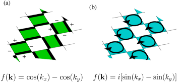 |
Returning to the table of possible pairing symmetries (Table 1) we therefore have two remaining options: the quadrupolar charge density waveAmitsuka02 (Fig. 8 (a)) and the orbital antiferromagnet(Fig. 8 (b)).Chandra02a ; Chandra02b , where both scenarios are consistent with our picture of as an incompressible Fermi liquid with strong antiferromagnetic fluctuations. Each order parameter has nodes, so that neither couples directly to the local charge density. Furthermore both incommensurate density waves couples weakly to uniform strain, and thus are both consistent with the observed insensitivityLuthi93 of the elastic response at . Recent uniaxial stress measurements suggests that the hidden order is sensitive to the presence of local tetragonal symmetry,Yokoyama02 a feature that can be explained within both frameworks for completely different reasons. In the orbital antiferromagnet the currents are equal in each basal directionChandra02b , whereas within the quadrupolar scenario it is known that some of the crystal-field states with tetragonal symmetry are quadrupolar.Santini00 Unfortunately the diamagnetic response cannot be used to discriminate between these two scenario, as the contribution from orbital antiferromagnetism is small compared to that associated with the gapping of the Fermi surface ().
At present, the key factor distinguishing the orbital antiferromagnet from the quadrupolar charge-density wave scenarios is the absence or present of time-reversal breaking. Because the local field distributions and strengths measured by NMR have not yet been observed by other methods, there is still uncertainty about these results. We note that it has been arguedKiss04 that the observation of a stress-induced momentYokoyama02 implies that the hidden-order breaks time-reversal symmetry; much as we would like to believe this, we note that this result can be attributed to a volume-fraction effect and thus is inconclusive. Both the quadrupolar charge density wave and the orbital antiferromagnet have nodes in their respective gaps, which should in principle be observable via photoemission and/or scanning tunnelling microscopy, though issues associated with the nature of the surface of this material remain to be resolved. However the quadrupolar charge density wave is not expected to lead to magnetic neutron scattering, and therefore detailed elastic measurements are critical for resolving the nature of the hidden order parameter.
IV Toy model for Anisotropic Particle-Hole Pairing
Next we explore a simple model for heavy electrons with antiferromagnetic spin fluctuations, and explore different orderings. We are motivated by experiment in our choice of the model. URu2Si2 undergoes a phase transition to a d-wave superconducting state at , and the pairing is understood to be mediated by antiferromagnetic spin fluctuations. The same model also encompasses orbital antiferromagnetism, quadrupolar CDW, and isotropic SDW.
We consider a simplified model for the heavy Fermi liquid, described by , where
describes the band of heavy electrons and
| (30) |
is the interaction between them. Here, is the Fourier transform of the local spin operator. . In this simplified model, we consider the indices to represent the pseudo-spin indices of the spin-orbit-coupled, heavy-electron band. We recall that we are working in an itinerant basis where the local physics (e.g. spin-orbit coupling) is absorbed into the composite quasiparticle states. Using the completeness relation we may rewrite this interaction as
Here we have rewritten the electron operators in a local basis, so that is the electron creation operator at site , is the number of sites in the lattice and is the spin interaction between sites and . We shall ignore the second term, which involves the heavily suppressed fluctuations in quasiparticle occupation at each site. The first term can be decoupled as
| (31) |
where , etc. The interaction potential can be expanded into partial waves,
| (32) |
where and . We require that the (isotropic) component be large and negative, reflecting strong on-site quasiparticle repulsion. This has the effect of suppressing isotropic particle-hole pairing. However this potential , for , could be attractive, which would then favour particle-hole pairing in higher angular momentum channels. Such higher angular momentum components are present due to anisotropy of the interaction , which occurs at sufficiently large values of where the underlying symmetry of the crystal becomes important.
For the purposes of a toy model, we shall assume in URu2Si2, nearest neighbour antiferromagnetic spin fluctuations (AFMSF) predominate, so that
| (33) |
where the form factor . With this approximation, the interaction in Eq.(31) is separable:
| (34) |
where
| (35) |
are the particle-hole operators and
| (36) | |||||
| (37) |
are form factors that transform under the point-group symmetry of the lattice. Since , the quantity inside the summation is symmetric under , and so, by doubling the prefactor and restricting the sum over to one-half the Brillouin zone, we assure that every term in the sum is independent.
This interaction is attractive and of equal magnitude in the four anisotropic channels. , , have s-like, d-like and p-like symmetry respectively. Notice that bond-variables are invariant under time reversal, and the imaginary pre-factors in have been chosen so that the form-factors respect this symmetry, i.e .
By carrying out a “Hubbard Stratonovich” decoupling of , we obtain
| (38) | |||||
Now the mean-field solution to this expression is determined by the saddle-point condition
| (39) |
In general, the density wave will condense at a primary wavevector . For a realistic model, may well be incommensurate, in which case, it will be accompanied by a family of corresponding that form a “star” of q-vectors under the point group. There will in general also be higher harmonics of . To illustrate the key ideas however, we shall assume a simple model in which a single dominates the density wave, i.e.
For this discussion, we shall also assume that the Fermi surface is “almost nested”, so that the Fermi surface can be divided into two equal parts or reduced Brillouin zones (RBZ): region I in which and region II in which . In perfectly nested Fermi surfaces are perfectly degenerate. For a square lattice and the reduced Brillouin zone is the diamond-shaped region bounded by .
The mean-field Hamiltonian is then
| (44) | |||||
| (45) |
where and . Here, is the wave vector for particle-hole pairing. Diagonalising the electronic part of the total Hamiltonian yields two bands,
| (46) | |||||
The mean field solution for pairing density in Eq.(39) is obtained by setting the variation of the free energy ,
| (47) | |||||
with respect to to zero. This yields the gap equation,
| (48) |
In the special case where condensation occurs in a single channel , this simplifies to
| (49) |
At , Equation (48) is essentially a Stoner criterion where
| (50) |
is the susceptibility associated with the hidden order parameter , measured at a wave vector .
Without details of the band-structure we can not predict which of the four order parameters will dominate. Some general comments are however in order. Although the pairing equation (48) does not involve any isotropic order parameter, the extended-s wave order parameter does have the same point-group symmetry as a pure s-wave and if it condenses, will tend to induce charge modulation. In a real heavy electron system, the effects of Coulomb interaction will renormalise the effective coupling constant for this channel, eliminating this order parameter from consideration. Of the remaining cases, corresponds to a q-CDW order and can be associated with spontaneous orbital or line currents between the Uranium atoms, as we shall now show.
Let us consider the current
| (51) |
from to along bond . Orbital order corresponds to a non-vanishing circulation of the current in a plaquette:
and, therefore, is of the form (Fig. 4 (a) ).
| (52) |
where is the position of the centre of the plaquette, and the indices label the corners of the plaquette, taking the sense of rotation to be anti-clockwise.
Now consider the evaluation of the bond variable . Taking the Fourier transform each electron field, we obtain
| (53) | |||||
| (54) | |||||
| (55) |
where we assumed . The current along a given bond is therefore
| (56) | |||||
| (57) |
Averaging the currents anti-clockwise around a plaquette centred at , we arrive at
| (58) |
where
| (59) | |||||
| (60) |
where we have used the notation and
(notice the ordering of the y and x terms). The form factor for orbital current order is thus a weighted mixture of and . Using Eq.(39) to simplify Eq. (60), we obtain a relation between the orbital current and gap,
| (61) |
where
In actual fact, the relative weight of the two channels in the orbital antiferromagnet is not an adjustable parameter. If we calculate the divergence of the current at a given node in the lattice, we find that
| (62) | |||||
| (63) | |||||
| (64) |
so the choice of vector determines the mix of and symmetry in the orbital antiferromagnet.
In an itinerant model the condition for instability into the hidden order phase will be given by the Stoner criterion already discussed () where so that typically at the transition where is a constant; this is the relation we used for the current in our earlier phenomenological treatment. The form factor corresponds to a quadrupolar charge density wave (q-CDW). The particular details of the conduction electron spectrum determine which order parameter has a higher critical temperature. For instance, if , and , which corresponds to a nested Fermi surface, then from Equation (49) the relation for is
| (65) |
Here we used . In this particular limit, we can explicitly verify that orbital antiferromagnetism has a higher than q-CDW. In the real material, the spectrum may differ greatly from this simple form, which may result in a preference of q-CDW over OAFM.
Our discussion in this section is based on a weak-coupling treatment of orbital antiferromagnetism, which is technically only valid in the vicinity of a nesting instability. Real heavy electron systems involve interactions of a size comparable with the band-width, in which the vicinity to nesting will no longer be a requirement. Practical modelling of these situations will require alternate strong-coupling methods, such as methods based on a Kondo lattice model. It is however interesting to note that that both symmetry and microscopic toy treatments appear to point to quadrupolar charge density wave and orbital antiferromagnetism as the leading contenders for hidden order in .
V Fluctuations and Nesting
The sharpness of the phase transition in URu2Si2 indicates that fluctuations do not make a significant contribution to thermodynamic properties. From the observed specific heat anomaly, the region of fluctuations is certainly smaller than , so that . This is an unusual situation in the general context of local moment magnetism, where broad fluctuation regions are generally seen in the specific heat anomaly. This result is sometimes taken to indicate that the hidden order involves a nested Fermi surface.Ikeda98 ; Sikkema96 However band structure calculations have not revealed any signs of a nested Fermi surface,Norman88 and it is difficult to see how such a condition might occur naturally in the complex band-structure of an f-electron system. Sharp mean-field transitions are generally taken as an indication of a large coherence length scale associated with fluctuations. In insulating systems (e.g. ferroelectrics) this arises from the long-range nature of the interaction. In superconductors and in nested charge density wave systems, the long coherence length is a consequence of the non-local order parameter response of the itinerant electron fluid.
So can the sharpness of the specific heat transition can be used in be used to infer the presence of nesting ? In fact, as we shall now see, a careful examination of the Ginzburg criterion for this system shows that while we may confirm that the ordering is itinerant in nature, the small size of the heavy electron Fermi energy means that we do not need to invoke nesting to understand that sharpness of the transition.
The Ginzburg criterion for a phase transition is given by
| (66) |
or in three dimensions,
| (67) |
Here is the lattice spacing, is the entropy associated with the phase transition and is the coherence length of the order parameter. Microscopically, is determined from the Gaussian fluctuation term in the order-parameter expansion of the free energy,
| (68) |
where and is a normalisation constant. The Gaussian coefficient in the integral is directly related to the static susceptibility of the order parameter
| (69) |
The relationship between the coherence length and microscopic quantities depends markedly on the underlying physics. In insulators, tends to be determined by the range of interaction of the order parameter, but in itinerant systems, it is determined by the non-local order-parameter polarisation that develops in the electron fluid.
For example, in a local-moment antiferromagnet, with interaction ,
| (70) |
When we expand around the unstable vector,
| (71) |
where is the Curie constant and the effective range of the interaction. With this form, we see that for insulating systems, the coherence length becomes the range of the interaction. For short-range interactions, this reason, the breadth of fluctuation region is generally large. In insulating systems, narrow fluctuation regimes are therefore associated with long-range interactions.
By contrast, in itinerant electron systems the order-parameter susceptibility generally takes the form
| (72) |
where is the strength of short-range interaction between electrons in the channel corresponding to the order parameter and takes the form given in (50). It is the momentum dependence of that determines the Ginzburg criterion in itinerant systems. To understand the role of nesting, let us consider a Fermi surface in which the departure from dispersion is measured by an energy scale , (e.g ) then the dispersion satisfies
| (73) |
so that the bare susceptibility (50) is given by
| (74) |
For and , this integral is logarithmically divergent at , and given by at finite temperatures. Finite modifies the Fermi functions in (74), so that
| (75) | |||||
| (76) |
so that
| (77) |
and the free energy expansion takes the form
| (78) |
so by comparing with (68), we see that for a nested system, the coherence length takes the “BCS” form
| (79) |
When , then we must replace in the Landau-Ginzburg expansion, i.e.
| (80) | |||||
| (81) |
from which we see that the coherence length is given by
| (82) |
where we have replaced , so loosely speaking, the absence of nesting replaces the coherence length by the geometric mean of the BCS coherence length and the lattice spacing.
Let us now return to our case, . Here, using the three dimensional form of the Ginzburg criterion, and taking , , so that
| (83) |
Suppose the fluctuation region is less than , i.e. , then a lower bound for the coherence length is
Clearly, the presence of the sixth power in the Ginzburg criterion, means that only modest coherence length is required to account for experiments. Were the hidden order strictly associated with the local moments, then we would expect , and clearly, the absence of fluctuations is sufficient to rule this case out. The high pressure magnetic phase transition does in fact show clear signs of Ising fluctuations, and in this region, it would appear that the ordering transition is indeed local in nature. However, we can account for the coherence length of the hidden order transition by appealing to itineracy, without nesting. By assuming that . Taking , consistent with the heavy mass and , we are clearly in the right range. From these arguments, we see that a correlation length of order lattice spacings is fully consistent with a system that is un-nested but itinerant. We conclude that the sharpness of the hidden order phase transition in only implies itineracy. Indeed, there are a number of heavy electron systems with sharp thermodynamic transitions and commensurate magnetic order, indicative of un-nested Fermi surfaces, such as Ott84 and .Geibel91 In each of these cases, it is most likely the itineracy alone that is responsible for the narrow fluctuation regime.
VI Discussion
The observed Fermi liquid behaviour for , the sharp nature of the transition and the large entropy loss point to the hidden order as a general density-wave with itinerant excitations formed from the local spin and orbital degrees of freedom of the uranium ions and f-electrons. Motivated by nuclear magnetic resonance measurements, we have expanded on our proposal (with J.A. Mydosh) of the hidden order as incommensurate orbital antiferromagnetism and have provided technical details for our predictions for elastic neutron scattering. Next we have turned to a microscopic description of the hidden order. After discussing symmetries and allowed particle-hole pairings in general terms, we studied the developing of these ordering in the setting of a toy single-band model within a weak-coupling approach. Within this framework, selection between q-CDW and OAFM ordering is not possible, though the situation may be different in the (experimentally relevant) strong-coupling regime. As discussed in Sec.III.2, density wave instabilities such as q-CDW and OAFM can account for the large entropy loss observed at the transition () if the density of states at the Fermi surface, , is large (as is the case in a heavy Fermi-liquid), and there is a substantial gapping of the Fermi surface.
The weak-coupling model we considered requires the nesting of a significant part of the Fermi surface. This requirement can be relaxed if the coupling is strong. Indeed it seems that a strong coupling description might be more appropriate for URu2Si2, since the transition temperature is an order of magnitude smaller than the gap unlike a weak coupling description where is more comparable with . Unfortunately here it is difficult to perform controlled calculations in this regime, and thus experiment is crucial for discerning between these two competing scenarios of quadrupolar charge density wave order and orbital antiferromagnetism. In Sec. II we studied the consequences of OAFM for the neutron scattering structure-factor and NMR at the Si and Ru sites. No particular microscopic model was assumed here, so the analysis is applicable for any coupling. NMR observations were used with our OAFM model to predict an incommensurate wavevector for orbital ordering which may be verified by neutron scattering measurements. To date, these predictions remain untested, as current experimental resolution is insufficient to observe the anticipated signal level from an OAFM.Bull02 ; Wiebe04 Here we identify a region of momentum space where elastic neutron scattering probes will clearly be able to distinguish between a spin density wave and an OAFM with current signal-noise levels. This prediction for orbital anferromagnetism remains a challenge for future experiments.
Our proposal of orbital antiferromagnetism is strongly motivated by the inhomogeneous line-broadening observed in ambient pressure NMR,Bernal01 and there are questions associated with this experiment that concern us greatly. In particular, the local fields measured via NMR in epoxied powdered samples are an order of magnitude larger than those probed by muon spin resonance or nuclear magnetic resonance in single-crystal ones. One interesting possibility is “motional narrowing”. The proposed orbital antiferromagnetic order is incommensurate and quite similar in its current patterns to a flux lattice of core-less vortices, where the absence of vortex cores weakens the pinning effect of disorder. In single domain crystals an incommensurate orbital antiferromagnet should then be weakly pinned, giving rise to large thermal motion.Blatter94 The probed local-fields will then be “motionally narrowed”, i.e their time-average will be significantly reduced in magnitude relative to their its static counterpart. One of the predictions of this scenario, is that the the muon or NMR linewidth will increase systematically with disorder - an effect that might be tested using radiation damage to systematically tune the disorder in a single sample.
Since we started working on this project, there have been a number of new experiments which may place further constraints on the nature of the hidden order in . In particular, recent magnetotransport measurementsBahnia05 indicate an unusually large Nernst signal in that develops at . This kind of behaviour has also been seen in the pseudogap phase of underdoped cuprate superconductors. In the case of the cuprate superconductors, this is most likely an effect of the Magnus force on the pre-formed pairs in the pseudogap. However, here, the absence of any superconductivity makes it far more likely that the giant Nernst effect seen here is a property of the quasiparticles in the presence of the hidden order parameter. These new results clearly place an important constraint on the microscopic nature of the order parameter.
Recent high magnetic field studiesKim03 have raised additional questions about the hidden order in . Application of high magnetic fields confirms that the hidden order persists to significantly higher values than does the remnant antiferromagnetism, affirming the two-phase scenario.Chandra02a Moreover the application of still higher fields leads to a profusion of new hidden order phases that may well cloak a field-induced quantum critical point. At the current time, it is not yet clear whether the proposed quantum critical point is a consequence of the loss of hidden order, or whether it might arise from the close vicinity to a quantum critical end point (as is the caseMillis02 with .)
The hidden order mystery in Uranium Ruthenium-2 Silicon-2 can be regarded as part of a much broader set of longstanding problems that our community faces in the context of highly correlated materials. Coexisting forms of hidden order, novel metallic states manifested by unusual resistance and magnetotransport properties, field-induced quantum phase transitions- each of these features, present in , are manifest themselves in a wide range of other strongly correlated materials, such as the cuprate superconductors, strontium ruthenate, magneto-resistance materials, and many other heavy electron systems. offers an alternative perspective on these problems, and optimistically, its ultimate solution will provide part of the key to understanding these broader questions.
Appendix A Spatial distribution of vector potential due to OAFM
Here we calculate the vector potential due to orbital order by summing up contributions from currents in all links. Consider first the contribution defined in Eq.(8) for links along . Performing the integral over gives
| (84) | |||||
where we have used the notation to denote the co-ordinates of the centre of the plaquette. For the link shown in Fig.4 we have
| (85) | |||||
The component of the vector potential is then . Similarly the vector potential in the links and ,
| (87) | |||||
| (88) | |||||
yield the component of the vector potential . The magnetic field follows straightforwardly from .
Acknowledgements.
We are very grateful to J.A. Mydosh for innumerable discussions on which have shaped our view on this subject. We have also benefitted greatly from interactions with W.J.L. Buyers particularly related to the experimental neutron scattering situation and the Ginzburg criterion in itinerant systems. Discussions with K. McEwen, B. Maple, B. Marston, P. Ong and I. Usshikin are also acknowledged. VT is supported by a Junior Research Fellowship from Trinity College, Cambridge. P. Chandra and P. Coleman are supported by the grants NSF DMR 0210575 and NSF DMR 0312495 respectively. P. Coleman acknowledges the hospitality of the Kavli Institute for Theoretical Physics, where part of this work was performed.References
- (1) B.I. Halperin and T.M. Rice in Solid State Physics; eds. F. Seitz, T. Turnbull, H. Ehrenreich, Vol.21, 116 (Academic, New York, 1968).
- (2) I. Affleck and J.B. Marston, Phys. Rev. B 37, 3774 (1988).
- (3) B.G. Kotliar, Phys. Rev. B 37, 3664 (1988).
- (4) A.A. Nersesyan and G.E. Vachnadze, J. Low. Temp. Phys. 77, 293 (1989).
- (5) H.J. Schulz, Phys. Rev. B 39, 2940 (1989).
- (6) S. Chakravarty, R.B. Laughlin, D.K. Morr and C. Nayak, Phys. Rev. B 63, 094503-1 (2001).
- (7) P. Lee, Physica C 408-410 5, (2004).
- (8) J.O. Fjaerestad and J.B. Marston Phys. Rev. B 65 125106 (2002); J.O. Fjaerestad, J.B. Marston and U. Schollwock, cond-mat/0412709.
- (9) S. Capponi, C. Wu and S. C. Zhang, Phys. Rev. B 70, 220505(R) (2004).
- (10) P. Chandra, P. Coleman, and J.A. Mydosh, Physica B 312-313, 397 (2002).
- (11) P.Chandra, P.Coleman, J.A.Mydosh, and V.Tripathi, Nature 417, 831 (2002).
- (12) J.A. Mydosh, P. Chandra, P. Coleman and V. Tripathi, Acta Polonius 34 659 (2003).
- (13) P. Chandra, P. Coleman, J.A. Mydosh and V. Tripathi, J. Phys. Cond. Mat. 15 S1965 (2003).
- (14) T.T.M. Palstra et al., Phys. Rev. Lett. 55, 2727 (1985).
- (15) Y.Miyako et al., J. Appl. Phys. 70, 5791 (1991).
- (16) A.P.Ramirez et al., Phys. Rev. Lett. 68, 2680 (1992).
- (17) A.De Visser et al., Phys. Rev. B 34, 8168 (1986).
- (18) T.T.M.Palstra, A.A.Menovsky, and J.A.Mydosh, Phys. Rev. B 33, 6527 (1986).
- (19) P. Chandra et al. Physica B 199 & 200, 426 (1994).
- (20) U.Walter et al., Phys. Rev. B 33, 7875 (1986).
- (21) T.E.Mason and W.J.L.Buyers, Phys. Rev. B 43, 11471 (1991).
- (22) C.Broholm, J.K. Kejms, W.J.L. Buyers, P. Matthews, T.T.M. Palstra, A.A. Menovsky, and J.A. Mydosh, Phys. Rev. Lett. 58, 1467 (1987).
- (23) C.Broholm et al., Phys. Rev. B 43, 12809 (1991).
- (24) W.J.L. Buyers, Physica B 223 9 (1996).
- (25) S.A.M.Mentink et. al, Phys. Rev. B 53, R6014 (1996).
- (26) N.H.van Dijk et. al, Phys. Rev. B 56, 14493 (1997).
- (27) F. Bourdarot et. al, Phys. Rev. Lett. 90, 061203-1 (2003).
- (28) T.E.Mason et. al, J. Phys. Cond. Mat. 7, 5089 (1995).
- (29) H.Amitsuka et. al, Phys. Rev. Lett. 83, 5114 (1999).
- (30) R.A.Fisher et. al, Physica B 163, 419 (1990).
- (31) G.M.Luke et. al, Hyperfine Int. 85, 397 (1994).
- (32) H. Amitsuka et. al, Physica B 326 418 (2003).
- (33) K. Matsuda et. al, Phys. Rev. Lett. 87, 087203 (2001).
- (34) G. Motoyama et. al Phys. Rev. Lett. 90 1664021 (2002)
- (35) B. Lüthi et. al, Phys. Lett. A175, 237 (1993).
- (36) e.g. R. Melcher, J. Appl. Phys. 41 1412 (1970).
- (37) A. Virosztek, K. Maki and B. Dora, Int. J. Mod. Phys. 16, 1667 (2002).
- (38) C.M. Varma and L. Zhu, cond-mat/0502344.
- (39) P. Santini and G. Amoretti, Phys. Rev. Lett. 73, 1027 (1994).
- (40) P. Santini and G. Amoretti, Phys. Rev. Lett. 85, 654 (2000).
- (41) H. Amitsuka et al. Physica B 312-3, 390 (2002).
- (42) A. Kiss and P. Fazekas, cond-mat/0411029.
- (43) V.P. Mineev and M.E. Zhitomirsky, cond-mat/0412055.
- (44) O.O. Bernal et al., Phys. Rev. Lett. 87, 1964-2-1 (2001).
- (45) K. Miyake, S. Schmitt-Rink and C.M. Varma, Phys. Rev. B 34, 6554 (1986).
- (46) N. Shah et al. Phys. Rev. B 61 564 (2000).
- (47) C. Schlichter, Principle of Magnetic Resonance, (Springer, Berlin, 1978).
- (48) M.J. Bull et al. Krakow Conference Proceedings.
- (49) C.R.Wiebe et al. Phys. Rev. B 69, 132418 (2004).
- (50) O.O.Bernal, M.E.Moroz, J.A.Mydosh, D.E.MacLaughlin, H.G.Lukefahr, and T.Gortenmulder (2004) (to be published).
- (51) Y.Kuramoto and K.Miyake, J. Phys. Soc. Jap. 59, 2831 (1990).
- (52) Y. Okuno and K. Miyake, J. Phys. Soc. Jap. 67 2469 (1998).
- (53) V.J.Emery, Phys. Rev. Lett. 58, 2794 (1987).
- (54) C. Nayak, Phys. Rev. B 62, 4880 (2000).
- (55) H. Ikeda and Y. Ohashi, Phys. Rev. Lett. 81, 3723 (1998).
- (56) M.N. Kiselev and F. Bouis, Phys. Rev. Lett. 82,5172 (1999); H. Ikeda and Y. Ohashi, Phys. Rev. Lett. 82, 5173 (1999).
- (57) M. Yokoyama et. al, J. Phys.Soc. Jap. bf71, 264 (2002).
- (58) A. E. Sikkema, W. J. L. Buyers, I. Affleck & J. Gan Phys. Rev. B54,9322-7 (1996).
- (59) M.R. Norman, T. Oguchi and A.J. Freeman Phys. Rev. B38, 11193-8. USA.(1988).
- (60) H. R. Ott, H. Rudigier, P. Delsing and Z. Fisk, Phys. Rev. Lett. 52, 1551-1554 (1984)
- (61) C. Geibel, C. Schank, S. Thies, H. Kitazawa, C. D. Bredl, A. B. M. Rau, A. Grauel, R. Caspary, R. Helfrich, U. Ahlheim, G. Weber and F. Steglich, Z. Phys. B 84, 1 (1991); M. Rau, A. Grauel, R. Caspary, R. Helfrich, U. Ahlheim, G. Weber and F. Steglich, Z. Phys. B 84, 1 (1991).
- (62) G. Blatter et al., Rev. Mod. Phys 66 1125 (1994).
- (63) K. Bahnia et al. Phys. Rev. Lett. 94 156405 (2005).
- (64) K.H. Kim et al. Phys. Rev. Lett. 256401 (2003); M. Jaime et al. Phys. Rev. Lett., 89 287201 (2002); N. Harrison et al. Phys. Rev. Lett., 90 096402 (2002).
- (65) A.J. Millis et al., Phys. Rev. Lett. 88 217204 (2002); S.A. Grigera et al. Science 294, 329 (2001); S.A. Grigera et al. Science 306 1154 (2004).