Transport anomalies in a simplified model for a heavy electron quantum critical point
Abstract
We discuss the transport anomalies associated with the development of heavy electrons out of a neutral spin fluid using the large- treatment of the Kondo-Heisenberg lattice model. At the phase transition in this model the spin excitations suddenly acquire charge. The Higgs process by which this takes place causes the constraint gauge field to loosely “lock” together with the external, electromagnetic gauge field. From this perspective, the heavy fermion phase is a Meissner phase in which the field representing the difference between the electromagnetic and constraint gauge field, is excluded from the material. We show that at the transition into the heavy fermion phase, both the linear and the Hall conductivity jump together. However, the Drude weight of the heavy electron fluid does not jump at the quantum critical point, but instead grows linearly with the distance from the quantum critical point, forming a kind of “gossamer” Fermi-liquid.
I Introduction
The past few years has seen a growth of interest in quantum phase transitions and the associated phenomenon of quantum criticality Continentino (1994); Sachdev (1999); Stewart (2001); Vojta (2003); Hertz (1976); Millis (1993); Si et al. (2001); Coleman and Pépin (2002); Coleman and Schofield (2005). Although quantum criticality develops at a zero-temperature phase transition, the ability of quantum criticality to profoundly modify the metallic properties of both d- and f-electron materials at a finite temperature has aroused intense interest. Heavy electron materials have played a particularly important role in the study of quantum criticality, for these systems lie at the brink of antiferromagnetic instabilities Stewart (2001), and they are readily tuned to an antiferromagnetic quantum critical point. In the approach to a heavy electron quantum critical point, the characteristic energy scale of both the Fermi liquid and the magnetic excitations appear to telescope to zero, as indicated by the appearance of scaling in inelastic neutron scattering, and the development of scaling in both the specific heat and resistivity, characterized by a single energy scale which goes to zero at the quantum critical point Schröder et al. (2000); Custers et al. (2003).
The standard model for the development of magnetism in a Fermi liquid, which describes the emergence of antiferromagnetism as a quantum spin density wave, is unable to account for the simultaneous collapse of both the Fermi and magnetic energy scales at quantum criticality Coleman and Pépin (2002). This suggests the need for a radically new mechanism for the emergence of magnetism in the heavy electron state. The solution of classical criticality required two steps: the formulation of a mean-field theory—provided by the Landau-Ginzburg theory—and then the application of the renormalization group to the fluctuations around the mean field. In the parallel study of quantum criticality, experiments suggest the need to search for a new class of mean-field theory that describes the emergence of magnetism in the heavy electron fluid. Various new approaches have been explored, including the idea of local quantum criticality Si et al. (2001), the notion that spin and charge separate at a quantum critical point Coleman and Pépin (2002) and the idea that magnetism develops out of the heavy fermion phase via an intermediate spin-liquid Senthil et al. (2004).
Part of the difficulty in understanding the heavy electron quantum critical point stems from the confluence of two separate physical phenomena. If we consider the passage from the ordered antiferromagnet into the heavy electron paramagnet there are two processes to consider:
-
-
the destruction of ordered magnetism and the associated divergence of spin fluctuations in both space and time, and
-
-
the formation of charged composite heavy electrons associated with the Kondo quenching of the fluctuating spin degrees of freedom.
While a complete theory of heavy electron quantum criticality needs to unify these two phenomena, Senthil et al. Senthil et al. (2004) have recently suggested examining models in which these separate phenomena occur in isolation. They take the view that these two transitions may actually be physically separated by an intermediate spin liquid. Even if this is not the case in practice, we can adopt their approach as a useful exercise to examine what changes in transport properties are expected to accompany the formation of charged heavy electrons.
One of the interesting pieces of physics at a QCP is that the spin degrees of freedom transform from localized, magnetically polarized objects, into mobile charged fermions. Very little is known about the transport anomalies that accompany this transformation. One proposal is that the Hall conductivity of the fluid will jump Coleman et al. (2001). At present, it is however, only possible to measure the change in the Hall conductivity at a magnetically-induced quantum phase transition where recent measurements suggest that the differential Hall conductivity jumps at a heavy electron quantum critical point Paschen et al. (2004). In this paper we examine the model for a heavy electron quantum critical point proposed by Senthil et al. and show how the d.c. transport properties show discontinuities at the transition. In particular the weak-field Hall effect and the Wiedemann-Franz ratio would jump. By contrast the optical Drude weight will be continuous through the transition and reflect a “gossamer” Fermi-liquid state.
II Large Kondo Lattice Model
Our basic starting model is the large- fermionic treatment of the Kondo Heisenberg model Coleman and Andrei (1989) with spin components labeled by Greek indices that run from to :
where
| (1) | |||||
| (2) | |||||
| (3) |
describe respectively the conduction band (), the on-site Kondo coupling between the local moment and the conduction band (), and the super-exchange between neighboring spin sites (). A vector potential has been introduced into the hopping matrix element: for a uniform vector potential, can be rewritten as , where the dispersion is the kinetic energy of the conduction electrons.
The physics of this model depends on the ratio of . In the Doniach scenario Doniach (1977) for the Kondo lattice, when , the spins antiferromagnetically order, and as is increased, the antiferromagnetic state undergoes a transition to heavy electron paramagnet. The detailed physics of this quantum phase transition is an unsolved problem. In a fermionic mean-field approach, valid in the large- limit, antiferromagnetism at small is replaced by a spin-liquid or valence-bond ground-stateColeman and Andrei (1989); Affleck and Marston (1988); Vojta and Sachdev (1999). Although this model does not permit us to examine the destruction of magnetism by the Kondo effect, it nevertheless affords the opportunity to examine the change in transport properties which accompany the formation of the heavy electron paramagnet. This is the topic of this paper.
When we formulate the Kondo Heisenberg model as a functional integral, we can decouple the Kondo and Heisenberg terms into a “slave boson” and an RVB gauge field, as follows: and where
Here the bond variable, , in the second term has been written as the product of an amplitude and phase term. The gauge field has been written in a form which assumes smooth variations about a uniform configuration. Fluctuations of this gauge field enforce the constraint that the spinon current flow between sites is zero. The mean-field theory of this model, requires an additional constraint term, as follows
so that variations in enforce the constraint , where is the number of f-electrons used to represent the large spin.
There are two mean-field phases of interest,
-
•
A uniform RVB spin liquid phase where , but assumes a uniform value. In this phase the spinons, represented by fermions are unconfined, and have a dispersion determined by .
-
•
The heavy electron phase, where and are both finite and uniform.
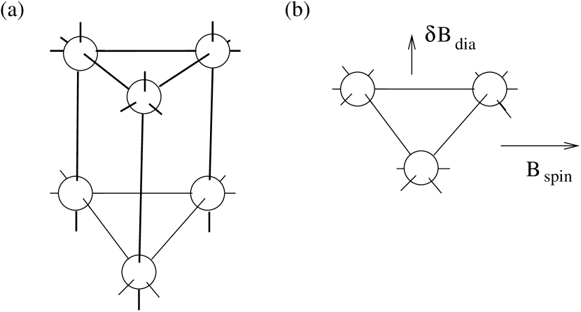
In this discussion, our main focus is on the transformation of the transport properties which occur at the second-order transition between these two phases. Strictly speaking, stabilization of the uniform RVB phase against instabilities to valence bond states, flux phases or plaquet states requires the presence of additional frustrating interactions, such as bi-quadratic Heisenberg couplings or spin-exchange terms around plaquets. Our discussion will assume that the Heisenberg terms are sufficiently frustrated to permit us to analyze a second-order between the two uniform phases. As a specific example, of such a model, we might consider a triangular crystal structure the type shown in Fig. 1, where frustration in the layers stabilizes the uniform solution. (To avoid a flux phase, we would need in addition, to include a ring exchange term around each rhombohedral plaquet.) It is conceptually easier in the model discussion we develop here, to take the two dimensional limit of this model. This has the conceptual advantage that magnetic field parallel to the layer couples only to the spin part of the Hamiltonian, so that we can separate the spin effects of field tuning from the diamagnetic effects associated with a field perpendicular to the plane.
To discuss the transport, we shall suppose that there is weak site disorder in the conduction electron fluid, and weak bond- disorder in the spin liquid to provide an elastic scattering mechanism.
III Effective action and the coupling of Gauge Fields
In the spin-liquid phase, where , the field decouples from the external vector potential. Just as the physical vector potential couples to currents of the conduction electrons, the field couples to “currents” of the f-spinons. For slow variations of these fields, the effective action obtained by integrating out the fermions, will take the form
| (4) |
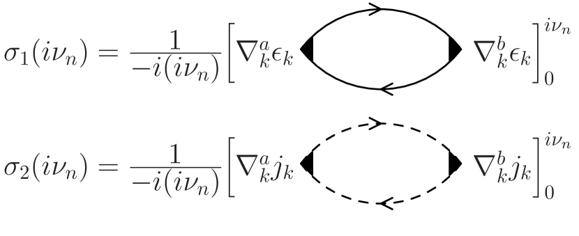
In the relaxation time approximation the conductivities
| (5) | |||||
| (6) |
describe the Drude response of the conduction and spinon fluid, to their respective gauge fields. The diagrams involved in the formal evaluation of these two quantities are shown in Fig. 2.
Although the vector potential and the fields couple in an essentially identical way to their respective fluids, is not an external field like , but fluctuates around a mean value . Fluctuations over this field guarantee the neutrality of the spin-liquid and preclude any flow of charge associated with the super-exchange couplings.
The transition between the spin-liquid and the heavy electron state involves the development of a small slave boson amplitude via a second-order phase transition. This occurs when the free energy, , satisfies
| (7) | |||||
| (8) |
where is the density of conduction electrons, and the estimate of the integral has been made, assuming that the band-width of the conduction electrons is much greater than the band-width of the spin liquid. So, when , the spin liquid becomes unstable with respect to the heavy electron state.
On the heavy electron side of this transition we have and the dispersion of the unconfined spinons and electrons now become mixed, forming a quasiparticle dispersion of the form
In general, the point where will in general be far from the Fermi surface, so that for small , the Fermi surfaces of the heavy electron fluid are essentially identical to conduction sea plus spin fluid. Nevertheless, the presence of a small slave boson amplitude leads to a non-trivial coupling between the physical vector potential and the gauge field , given by
| (9) |
To understand this coupling, consider the physical electromagnetic gauge transformations in the heavy electron phase. We can always choose a gauge where is real. In the heavy electron phase the hybridization between the f-spinons and conduction electrons given by , means that invariance of the Lagrangian only occurs if one carries out a single gauge transformation applied to both the f- and conduction fermions, i.e. the Lagrangian is only invariant under a single joint gauge transformation
| (10) |
This implies that when we expand the mean-field free energy in and , the free energy will be strictly a function of . So, to quadratic order in the fields, the full Lagrangian for the gauge field couplings is
| (11) | |||||
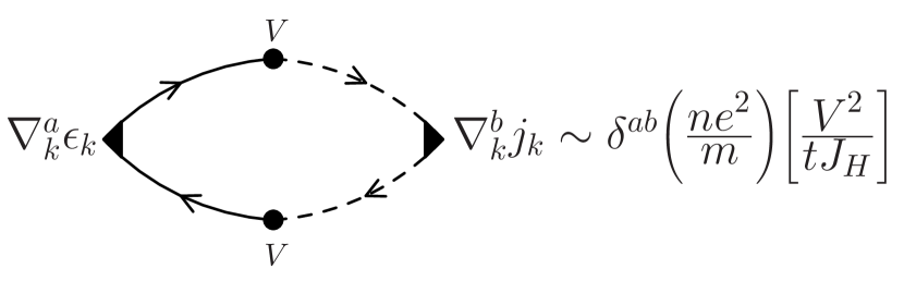
The coupling term between the two fields is given by the diagram shown in Fig. 3. Here and are respectively, the number density and effective mass of the conduction electrons, so that . In Eq. (11) we see that that both gauge fields, and , have developed a mass so that, at first sight, both the conduction fluid and the spin liquid have becomes superfluids. However, the linear coupling term between them ensures that, at long times, adapts to the value which minimizes the Free energy. It is this term that gives charge to the f-electrons so that the supercurrents of conduction and f-electrons mutually screen one-another. From the Gaussian coefficient of , we see that the propagator associated with the field is
| (12) |
indicating that the characteristic response rate of this field is given by
| (13) |
This sets the rate at which the supercurrents in the f- and conduction fluid adapt to screen one another. On time-scales longer than , the fluid is a heavy paramagnet.
One of the interesting consequences of the spin fluid acquiring a charge, is that the d.c. conductivity of the fluid must jump at the transition from spin to heavy electron liquidHoughton et al. (2002). When the spin liquid is neutral (the phase), the d.c. conductivity is simply given by the conduction electron component
| (14) |
However, once the spins acquire a charge in the heavy electron phase then the spinon fluid contributes directly to the D.C. conductivity
| (15) |
By contrast, we expect the thermal conductivities to be unchanged by the transition, because thermal currents of the spin liquid do not couple to the gauge fields. If and are the thermal conductivities of the conduction and spin fluids just before the transition, then the thermal conductivity of the heavy electron fluid will be given by on either side of the transition. From this discussion, we see that at transition from heavy electron fluid to spin liquid the Wiedemann-Franz ratio will jump from the standard value
| (16) |
in the heavy electron fluid, to the larger value
| (17) |
when the spin liquid becomes neutral.
We can calculate the jump in the d.c. conductivity directly by integrating out the field from Eq. (11). This gives
| (18) | |||||
| (19) |
where
| (20) |
is the renormalized conductivity. In this expression we have have omitted terms of order in the denominator of the second term. From this, we see that the optical conductivity acquires a new Drude peak at low energies, of width , weight . The zero frequency limit of this expression is indeed .
IV Jump in the Hall conductivity
To discuss the Hall conductivity, we need to consider the response of the system to crossed magnetic and electric fields which implies that we must consider the cubic interaction terms between the gauge fields. The Hall response requires us to to consider configurations of the vector potential containing a spatially uniform electric component, and a time-independent magnetic component , such that and ,
| (21) |
where is the residual “probe” part of the vector potential that is neither constant in space or time. In Fourier space,
| (22) |
where is the field used to probe the current. We also need to consider the analogous gauge fields that constrain the circulating currents in the spin liquid. The crossed gauge fields will now introduce a cubic term
| (23) | |||||
where . The coefficients and are related to the three-point current fluctuations of the conduction and spin fluids respectively,
| (24) | |||||
| (25) | |||||
Here the currents,
| (26) | |||||
| (27) |
are the “paramagnetic” current fluctuations of the conduction electrons and spin liquid, respectively. In an isotropic conduction fluid, where the Hall conductance gauge invariance requires that
| (29) |
so that we can identify the coefficient of the Hall conductance
| (30) |
In the spin liquid phase, the absence of any coupling between the two gauge fields guarantees that is the Hall response of the combined system. Similarly, it can be shown that
| (31) |
describes the analogous quantity for the spin liquid. In a simple relaxation time approximation, the above coefficients can be related to Fermi surface integrals of the quasiparticle mean-free path around the two dimensional Fermi surface, given by Ong (1991)
| (32) |
where and are the mean-free paths of the conduction and spin quasiparticles respectively. Now suppose we cross through the quantum phase transition into the heavy electron paramagnet. In this case, close to the transition, when integrate out the fluctuations over , we must replace by its expectation value
| (33) |
The renormalized cubic term is then given by
| (34) |
where
| (35) |
But in the long-wavelength, low frequency limit , so that in this limit and
| (36) |
In other words, we expect the Hall conductivity of the heavy electron fluid to be
| (37) |
so that the Hall conductivity jumps by an amount . This jump in the Hall response can be traced back to the fact that the previously neutral heavy-electron currents now become charged. At a zero field quantum critical point, the linear Hall current induced by a tiny, but fixed field will actually jump.
V Discussion
In this paper, we have studied a simplified model for a heavy electron quantum phase transition, involving a transition from a metal plus decoupled spin liquid, to a heavy electron fluid in which the fermionic spin excitations develop charge. Although our model is grossly over-simplified, it does illustrate how the development of charged heavy electrons out of the spin fluid is expected to affect the transport.
There are a number of interesting questions and observations that emerge from our model treatment.
-
•
The primary conclusion from our study is that the d.c. electrical conductivities (both longitudinal and Hall components) are expected to jump discontinuously at a quantum critical point between a heavy fermion metal and a spin liquid. The key ingredient in this transition is the sudden appearance of resonant levels at each site in the lattice which scatter the conduction electrons.
-
•
Our simple model assumed a separation between the spin and orbital parts of the magnetic field. Real heavy electron systems exhibit strong spin orbit coupling, so that the idealized separation between the spin and orbital parts of the magnetic field can not in general, be made. Nevertheless, the discontinuities we have found should be a general feature of any transition where the f-spin excitations suddenly develop a charge.
-
•
If we contrast our results with those anticipated in a spin density wave transformation of the Fermi surface, we note that here the magnetic order will couple linearly to the conductivity and to the Hall conductivity, so that gradual evolutions in the Hall constant at the quantum phase transition are expected in the limit of weak magnetic fields. Thus a jump in the Hall conductivity is a sign that the order parameter is intimately connected with the formation of new, coherent propagating charged quasiparticles.
Acknowledgements.
The authors would like to thank the hospitality of the Max Planck Institute for Complex Systems, Dresden, the Aspen Center for Physics and the Kavli Institute for Theoretical Physics, Santa Barbara, where part of the work in this article was carried out. This work was supported by NSF grants DMR 0312495 (PC) and DMR 0213818 (JBM), The Royal Society and Leverhulme Trust (AJS). This research was also supported in part by the National Science Foundation under Grant No. PHY99-0794. We would like to thank Dr. Silke Paschen for discussing her measurements on heavy electron materials prior to publication.References
- Continentino (1994) M. A. Continentino, Phys. Rep. 239, 179 (1994).
- Sachdev (1999) S. Sachdev, Quantum Phase Transitions (Cambridge University Press, Cambridge, UK, 1999).
- Stewart (2001) G. R. Stewart, Rev. Mod. Phys. 73, 797 (2001).
- Vojta (2003) M. Vojta, Rep. Prog. Phys. 66, 2069 (2003).
- Hertz (1976) J. A. Hertz, Phys. Rev. B 14, 1165 (1976).
- Millis (1993) A. J. Millis, Phys. Rev. B 48, 7183 (1993).
- Si et al. (2001) Q. Si, S. Rabello, K. Ingersent, and L. Smith, Nature 413, 804 (2001), eprint cond-mat/0011477.
- Coleman and Pépin (2002) P. Coleman and C. Pépin, Physica B 312-313, 383 (2002), eprint cond-mat/0110063.
- Coleman and Schofield (2005) P. Coleman and A. J. Schofield, Nature 433, 226 (2005).
- Schröder et al. (2000) A. Schröder, G. Aeppli, R. Coldea, M. Adams, O. Stockert, H. v. Löhneysen, E. Bucher, R. Ramazashvili, and P. Coleman, Nature 407, 351 (2000).
- Custers et al. (2003) J. Custers, P. Gegenwart, H. Wilhelm, K. Neumaier, Y. Tokiwa, O. Trovarelli, C. Geibel, F. Steglich, C. Pepin, and P. Coleman, Nature 424, 524 (2003).
- Senthil et al. (2004) T. Senthil, M. Vojta, and S. Sachdev, Phys. Rev. B 69, 035111 (2004).
- Coleman et al. (2001) P. Coleman, C. Pépin, Q. Si, and R. Ramazashvili, J. Phys.: Condens. Matter 13, R723 (2001), eprint cond-mat/0105006.
- Paschen et al. (2004) S. Paschen, T. Lühmann, S. Wirth, P. Gegenwart, O. Trovarelli, C. Geibel, F. Steglich, P. Coleman, and Q. Si, Nature 432, 881 (2004).
- Doniach (1977) S. Doniach, Physica B 91, 231 (1977).
- Coleman and Andrei (1989) P. Coleman and N. Andrei, J. Phys.: Condens. Matt. 1, 4057 (1989).
- Affleck and Marston (1988) I. Affleck and J. B. Marston, Phys. Rev. B 37, R3774 (1988).
- Vojta and Sachdev (1999) M. Vojta and S. Sachdev, Phys. Rev. Lett. 83, 3916 (1999).
- Houghton et al. (2002) A. Houghton, S. Lee, and J. B. Marston, Phys. Rev. B 65, R20503 (2002). The apparent violation of the Wiedemann-Franz law in the doped Fermi liquid phase reported in this paper is eliminated in a self-consistent mean-field calculation that allows the internal gauge field to relax. The violation remains at half-filling, however, as the spin-liquid conducts heat but no charge.
- (20) At first sight, our result appears to give a slight violation of the optical sum rule, since now . However, this can be traced back to the fact that we have not allowed for the slight renormalization of the dissipative part of Eq. (9 ) that is required in order to keep the high frequency coefficient of unchanged in (11). This small change means that the weight for the low frequency Drude peak is transfered from high frequencies of order .
- Ong (1991) N. P. Ong, Phys. Rev. B 43, 193 (1991).
- (22) Recent work by J. Fenton and A. J. Schofield (to be published) has shown that the magnetic field region where such a weak-field response might be observed collapses to zero at spin-density wave transition. At finite magnetic fields the Hall number will jump at a SDW transition but with a magnitude proportional to the applied field i.e. very different from the magnitude of the discontinuity in Hall number we have shown here which is independent of magnetic field.