Schwinger Boson approach to the fully screened Kondo model.

Abstract

We apply the Schwinger boson scheme to the fully screened Kondo model and generalize the method to include antiferromagnetic interactions between ions. Our approach captures the Kondo crossover from local moment behavior to a Fermi liquid with a non-trivial Wilson ratio. When applied to the two impurity model, the mean-field theory describes the ”Varma Jones” quantum phase transition between a valence bond state and a heavy Fermi liquid.

Recently, there has been a broad growth of interest in the behavior of heavy electron materials at a magnetic quantum critical pointreview . Several observations can not be understood in terms of the established Moriya Hertz theory of quantum phase transitionsmoriya ; hertz ; millis , including the divergence of the heavy electron massescusters , the near linearity of the resistivityhilbert1 ; mathur ; malte ; steglich and $E/T$ scaling in inelastic neutron spectraschroeder . The origins of this failure are linked to the competition between the Kondo effect and antiferromagnetism and may indicate the emergence of new kinds of excitationreview ; si ; senthil ; pepin05

In this letter, we show how to unify the Arovas Auerbacharovas description of quantum spin systems with the physics of the Kondo model by using Luttinger Ward techniques and a Schwinger boson spin representation. Our goal is to develop a large-$N$ expansion that contains the physics of antiferromagnetism and the Kondo effect in the leading approximation. Traditional pseudo-fermion abrikosov ; read ; auerbach representations of the spin are ill-suited to a description of local moment magnetism. By contrast, a Schwinger boson scheme works well for magnetism, but to date, has not been successfully applied to the fully screened Kondo model. We use a method co-invented by one of us (OP)parcollet97a in which the Kondo effect is captured in a large $N$ Schwinger boson scheme using a multichannel Kondo model where the number $K=kN$ of screening channels scales extensively with $N$. By tuning the number $n_{b}$ of Schwinger bosons from $n_{b}<K$ to $n_{b}>K$, one is able to describe both the overscreened and underscreened Kondo models, however, difficulties were encountered in the past work that appeared to prevent the treatment of the perfectly screened case, $n_{b}=K$. In this letter, we show how these difficulties are overcome.

Consider the multichannel Kondo impurity model,

$$\mathcal{H} = \sum_{\vec{k},\nu,\alpha}\epsilon_{\vec{k}}c^{{}^{\dagger}}_{\vec{k}\nu\alpha}c_{\vec{k}\nu\alpha}+H_{I}-\lambda(n_{b}-2S),$$ (1)

$$H_{I} = \frac{J_{K}}{N}\sum_{\nu\alpha\beta}\psi^{{}^{\dagger}}_{\nu\alpha}\psi_{\nu\beta}b^{\dagger}_{\beta}b_{\alpha}.$$ (2)

Here $c^{{}^{\dagger}}_{\vec{k}\nu\alpha}$ creates a conduction electron of momentum $\vec{k}$, channel index $\nu\in[1,K]$, spin index $\alpha\in[-j,j]$, where $N=2j+1$ is even. $\psi^{\dagger}_{\nu\alpha}=\frac{1}{\sqrt{{\cal N}_{s}}}\sum_{{\bf{k}}}c^{\dagger}_{{\bf{k}}\nu\alpha}$ creates an electron in the Wannier state at the origin, where ${\cal N}_{s}$ is the number of sites in the lattice. The operator $b^{\dagger}_{\alpha}$ creates a Schwinger boson with spin index $\alpha\in[-j,j]$. The local spin operator is represented by ${S}_{\alpha\beta}=b^{{}^{\dagger}}_{\alpha}b_{\beta}-\delta_{\alpha\beta}/N$ and the system is restricted to the physical Hilbert space by requiring that $n_{b}=\sum_{\alpha}b^{{}^{\dagger}}_{\alpha}b_{\alpha}=2S$. The final term in $H$ contains a temperature-dependent chemical potential $\lambda(T)$ that implements the constraint $\langle n_{b}\rangle=2S$. We will examine the fully screened case $2S=K$, taking the large $N$ limit where $N\rightarrow\infty$ keeping $k=K/N$ fixed.

We begin by factorizing the interaction in terms of auxilliary Grassman field $\chi_{\nu}$,

$$H_{I}\rightarrow\sum_{\nu\alpha}\frac{1}{\sqrt{N}}\left[(\psi^{\dagger}_{\nu\alpha}b_{\alpha})\chi^{\dagger}_{\nu}+{\rm H.c.}\right]+\sum_{\nu}\frac{\chi^{\dagger}_{\nu}\chi_{\nu}}{J_{K}}.$$ (3)

Following the steps outlined by us in earlier workindranil2 , we now write the Free energy as a Luttinger Wardluttinger2 functional of the one particle Green’s functions,

$$F[{\cal G}]=T\ {\hbox{Str}}\left[\ln\left(-{\cal G}^{-1}\right)+({\cal G}_{0}^{-1}-{\cal G}^{-1}){\cal G}\right]+Y[{\cal G}]$$ (4)

where $\hbox{Str}[A]={\hbox{Tr}}[A_{B}]-{\hbox{Tr}}[A_{F}]$ is the graded (super) trace over the Matsubara frequencies, internal quantum numbers of the bosonic (B) and fermionic (F) components of $A$. ${\cal G}_{0}$ is the bare propagator and ${\cal G}={\rm Diag}[\underline{G}_{b},\ \underline{G}_{\chi},\ \underline{G}_{c}]$, the fully dressed propagator, where

$$\underline{G}_{b}(i\nu_{n}) = [{i\nu_{n}+\lambda-\Sigma_{b}(i\nu_{n})}]^{-1}\delta_{\sigma\sigma^{\prime}},$$ (5)

$$\underline{G}_{\chi}(i\omega_{n}) = [{-J_{K}^{-1}-\Sigma_{\chi}(i\omega_{n})}]^{-1}\delta_{\nu\nu^{\prime}},$$ (6)

$$\underline{G}_{c}(i\omega_{n}) = [{G_{c0}^{-1}(i\omega_{n})-\Sigma_{c}(i\omega_{n})}]^{-1}\delta_{\sigma\sigma^{\prime}}\delta_{\nu\nu^{\prime}}.$$ (7)

$\Sigma(i\omega_{n})={\cal G}_{0}^{-1}-{\cal G}^{-1}$ denotes the corresponding self-energies. $G_{c0}(i\omega_{n})=\sum_{k}\frac{1}{i\omega_{n}-\epsilon_{k}}$ is the bare conduction electron Green’s function. The quantity $Y[{\cal G}]$ is the sum of all closed-loop two-particle irreducible skeleton Feynman diagrams. In the large $N$ limit, we take the leading $O(N)$ contribution to $Y$ (Fig. 1).

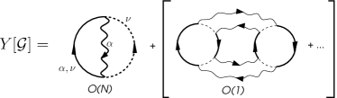
Figure 1: Leading contributions to $Y[{\cal G}]$ in $1/N$ expansion. Solid, dashed and wavy lines respectively represent $G_{c}$, $G_{\chi}$ and $G_{b}$. Each vertex is associated with a factor $i/\sqrt{N}$. Bracketed terms are dropped in the large $N$ limit.

The variation of $Y$ with respect to ${\cal G}$ generates the self-energy $\delta Y/\delta{\cal G}=\Sigma$, which yields $\Sigma_{c}(\tau)=\frac{1}{N}G_{\chi}(-\tau)G_{b}(\tau)$. Since $\Sigma_{c}$ is of order $O(1/N)$ we can use the bare conduction propagator $G_{c0}$ inside the self-consistent equations for $\Sigma_{\chi}(\tau)=G_{b}(\tau)G_{c0}(-\tau)$ and $\Sigma_{b}(\tau)=-kG_{\chi}(\tau)G_{c0}(\tau)$. In terms of real frequencies, these expressions become

$$\Sigma_{\chi}(\omega-i\delta) = -\int\frac{d\nu}{\pi}\left[h_{F}(\nu)G_{c0}^{\prime\prime}(\nu)G_{b}(\omega+\nu)\right.$$ (8)

$$+ \left.h_{B}(\nu)G_{b}^{\prime\prime}(\nu)G_{c0}^{*}(\nu-\omega)\right]$$ (9)

$$\Sigma_{b}(\nu-i\delta) = k\int\frac{d\omega}{\pi}h_{F}(\omega)\left[G_{c0}^{\prime\prime}(\omega)G_{\chi}(\nu-\omega)\right.$$ (10)

$$+ \left.G_{\chi}^{\prime\prime}(\omega)G_{c0}(\nu-\omega)\right]$$ (11)

where $G(\omega)\equiv G(\omega-i\delta)$ and the primed variables denote the real and imaginary parts of $G$. We use the notation $h_{B,F}(\omega)=\frac{1}{2}\pm n_{B,F}(\omega)$ where $n_{B,F}(\omega)=(e^{\beta\omega}\mp 1)^{-1}$ are the Bose and Fermi occupation numbers. The constraint $n_{b}=2S$ now becomes $\int\frac{d\nu}{\pi}n_{B}(\nu)G^{\prime\prime}_{b}(\nu)=\frac{2S}{N}$.

The original work in parcollet97a ; parcollet2 focussed primarily on the case of the overscreened Kondo model, where $K>2S$. The perfectly screened case where $K=2S$ presented two difficulties. First, the phase shift associated with the Kondo model is $\pi/N$, which vanishes in the large $N$ limit. Second, the requirement that $K=2S$ appeared extremely stringent, the slightest deviation from this condition apparantly leading to underscreened or overscreened behavior at low temperatures.

There are two new observations that enable us to now avoid these difficulties. First, the perfectly screened case where $2S=K$ is a stable “filled shell” singlet configuration of the spins. In strong-coupling, this stable ground-state corresponds to a singlet “rectangular” Young tableau representations of $SU(N)$. andrei1 ; andrei2 . In the gauge theory description of the Kondo model, this stability manifests itself as a gap in the Schwinger boson and $\chi$ fermion spectrum. When the chemical potential, $\lambda$ lies within this gap, the ground-state Schwinger boson occupancy locks into the value $n_{b}=K=2S$ (Fig. 2a).

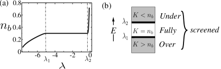
Figure 2: (a) Schematic variation of occupancy as a functional of boson chemical potential $\lambda$ in the ground-state. (b) Gap in spinon spectrum develops in the fully screened Kondo state.

The gap in the gauge particle spectrum has the effect of “confining” these excitations, so that the low energy physics only involves the elastic scattering of the conduction electrons off the Kondo singlet. From this perspective, the fully screened Kondo model is a kind of “spinon insulator” in this large-$N$ description, while over and underscreening develop when the spin-chemical potential is in the “valence” and “conduction” bands respectively ( Fig. 2 (b)). A second aspect to the problem concerns the scattering phase shift. Although the conduction phase shift is $\pi/N$, its effect on the thermodynamics is enhanced by the $N$ spin components and the $K$ scattering channels, producing an order $O(N\times K/N)\equiv O(N)$ effect in the mean field theory. Moreover, we can identify exact Ward identitiesindranil2 which give rise to a sum rule relating the scattering phase shift of the conduction electrons $\delta_{c}={\rm Im}\ln\bigl{[}1-{g}_{c0}(0-i\delta)\Sigma_{c}(0-i\delta))\bigr{]}$ to the phase shift $\delta_{\chi}={\rm Im}\ \ln(1+J_{K}\Sigma_{\chi}(0-i\delta))$ associated with the $\chi$ fermions, $\delta_{c}=\frac{1}{N}\delta_{\chi}$. The confined nature of the $\chi$ fermions means that $\delta_{\chi}=\pi$ in the ground-state, which guarantees that the Friedel sum rule $\delta_{c}=\pi/N$ is satisfied in this Schwinger boson scheme.

In the large $N$ limit the entropyindranil2 is given by

$$\frac{S(T)}{N}=\int\frac{d\omega}{\pi}\left\{\frac{dn_{B}(\omega)}{dT}\left[{\rm Im}\ln(-G_{b}^{-1})+G^{\prime}_{b}\Sigma^{\prime\prime}_{b}\right]+k\frac{dn_{F}(\omega)}{dT}\left[{\rm Im}\ln(-G_{\chi}^{-1})+G^{\prime}_{\chi}\Sigma^{\prime\prime}_{\chi}-G^{\prime\prime}_{c0}\tilde{\Sigma}^{\prime}_{c}\right]\right\}$$ (12)

(where the frequency labels $\omega$ in the integrand have been suppressed), and

$$\tilde{\Sigma}_{c}(\omega-i\delta)=N{\Sigma}_{c}(\omega-i\delta)=-\int\frac{d\nu}{\pi}\left[h_{F}(\nu)G_{\chi}^{\prime\prime}(\nu)G_{b}(\omega+\nu)\right.+\left.h_{B}(\nu)G_{b}^{\prime\prime}(\nu)G_{\chi}^{*}(\nu-\omega)\right]$$ (13)

is the rescaled conduction self-energy. At low temperatures, the gap in the boson and $\chi$ fermion spectrum means that only the conduction electron contribution dominates the entropy, and this is the origin of the Fermi liquid behavior. We can also calculate the local magnetic susceptibility

$$\chi_{\rm loc}(T)=-2N\int\frac{d\omega}{\pi}h_{B}(\omega)G^{\prime}_{b}(\omega)G^{\prime\prime}_{b}(\omega)$$ (14)

where we have taken the magnetic moment of the local impurity to be $M=\sum_{\sigma}\tilde{\sigma}b^{\dagger}_{\sigma}b_{\sigma}$, where $\tilde{\sigma}={\rm sign}(\sigma)$. Note in passing that the dynamic counterpart $\langle S(t)S(0)\rangle$ vanishes exponentially due to the gap in the bosonic spectral functions, the $1/t^{2}$ term characteristic of a Fermi liquid only appearing at the next order in $1/N$.

Figure 3: Showing temperature dependence of (a) impurity magnetic susceptibility and (b) specific heat capacity in the fully screened Kondo model for $k=0.3,\ 0.5,\ 0.7$ (with the Kondo temperature given by $T_{K}=De^{-2D/J_{K}}$, $D$ being the electron bandwidth). Inset calculated Wilson ratio.

We have numerically solved the self-consistent equations (8) for the self-energy by iteration, imposing the constraint at each temperature. Fig. 3. shows the temperature dependent specific heat coefficient $\frac{C_{V}}{T}=\frac{dS}{dT}$ and the full magnetic susceptibility $\chi(T)$. There is a smooth cross-over from local moment behavior at high temperatures $\chi\sim n_{b}(1+n_{b})/T$, to Fermi liquid behavior at low temperatures. From a Nozieres-Blandin description of the local Fermi liquidblandin (where channel and charge susceptibility vanish), we deduce the Wilson ratio

$$W=\frac{\chi/\gamma}{\chi_{0}/\gamma_{0}}=\frac{(1+k)}{1-\frac{1}{N^{2}}}.$$ (15)

This form is consistent with Bethe Ansatz resultsandrei1 . We may also derive this result by applying Luttinger-Ward techniquesyoshimori to our model. Our large $N$ approximation reproduces the limiting large $N$ behavior of this expression, $W=1+k$, in other words, the local Fermi liquid is interacting in this particular large $N$ limit.

To see how our method handles magnetic correlations, we have applied it to a two-impurity Kondo model,

$$H=\sum_{\vec{k},\nu,\alpha}\epsilon_{\vec{k}}c^{{}^{\dagger}}_{\vec{k}\nu\alpha}c_{\vec{k}\nu\alpha}+H_{K}(1)+H_{K}(2)-\frac{J_{H}}{N}B^{\dagger}_{12}B_{12},$$ (16)

where $H_{K}(i)$ is the Kondo hamiltonian for impurity $(i)$ and the antiferromagnetic interaction between the two moments is expressed in terms of the boson pair operator $B_{12}=\sum_{\sigma}\tilde{\sigma}b_{1\sigma}b_{2-\sigma}$. $H$ is invariant under spin transformations in the symmetry group SP (N) (N-even)readsachdev91 . We now factorize the antiferromagnetic interactionarovas ,

$$-\frac{J_{H}}{N}B^{\dagger}_{12}B_{12}\rightarrow\bar{\Delta}B_{12}+B^{\dagger}_{12}\Delta+\frac{N\bar{\Delta}\Delta}{J_{H}}.$$ (17)

Boson pairing is associated with the establishment of short-range antiferromagnetic correlations. Once $\Delta$ becomes non-zero, the local gauge symmetry is broken, and the Schwinger bosons propagate from site to site. In this “Higg’s phase” the $\chi$ fermions also delocalize, giving rise to a mobile, charged yet spinless excitation that is gapped in the Fermi liquid. Loosely speaking, these excitations are mobile Kondo singlets or “holons”. Since the paired Schwinger bosons interconvert from particle to hole as they move, they only induce holon motion within the same sublattice. In the special case of two-impurity model, so long as the net coupling between the spins is antiferromagnetic, the holons will remain localized.

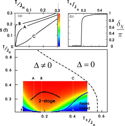
Figure 4: Phase diagram for the two-impurity Kondo model showing the boundary where boson pairing develops. Color coded contours delineate the entropy around the Varma Jones fixed point. Black line indicates upper maximum in specific heat, blue line, lower maximum in specific heat where cross-over into the Fermi liquid takes place. Inset - (a) entropy for various values of $T_{K}/J_{H}$ (b) showing dependence of $\delta_{\chi}$ on $T_{K}/J_{H}$ at a temperature $T/T_{K}=0.02$.

Under these assumptions, we can adapt the single impurity equations to the two-impurity model by replacing

$$G_{b}(\omega)\rightarrow\tilde{G}_{b}(\omega)=\left(G_{b}(\omega)^{-1}-|\Delta|^{2}G_{b}(-\omega)^{*}\right)^{-1}$$ (18)

in the integral equations. We must also impose self-consistency $\Delta=-J_{H}\langle B_{12}\rangle$, or

$$\frac{1}{J_{H}}=-2\int\frac{d\omega}{\pi}h_{B}(\omega){\rm Im}\left(\frac{1}{G_{b}^{-1}(\omega)G_{b}^{-1}(-\omega)^{*}-|\Delta|^{2}}\right)$$ (19)

We have self-consistently solved the integral equations with the modified boson propagator. Using the entropy as a guide, we are able to map out the large $N$ phase diagram for this model(Fig. 4.).

We find that the development of $\Delta\neq 0$ preserves the linear temperature dependence of the entropy at low temperatures, indicating Fermi liquid behavior. However, as the $J_{H}$ increases, the temperature range of Fermi liquid behavior collapses towards zero, vanishing at a quantum critical point where $J_{H}=J_{c}$. For $J_{H}>J_{c}$, Fermi liquid behavior re-emerges, but the phase shift $\delta_{\chi}$ is found to have jumped from $\pi$ to zero, indicating a collapse of the Kondo resonance. The entropy develops a finite value at the quantum critical point which is numerically identical to one half the high temperature entropy of a local moment, $(N/2)[(1+n_{b})\ln(1+n_{b})-n_{b}\ln n_{b}]$. Similar behavior occurs at the “Varma Jones” fixed pointvarma ; jones ; gan in the $N=2$ two-impurity model when the conduction band is particle-hole symmetric. We can in fact identify two maxima in the specific heat, indicating that as in the $N=2$ Varma Jones fixed point, the antiferromagnetic coupling generates a second set of screening channels, leading to a two-stage quenching process.

The survival of the Varma Jones fixed point at large $N$ in the absence of particle hole symmetry is a consequence of the two impurity Friedel sum rule which tells us that

$$(\delta_{+}+\delta_{-})=\frac{2\pi}{N}$$ (20)

where $\delta_{\pm}$ are the even and odd parity scattering phase shifts. For $N=2$, this condition is satisfied with $\delta_{+}=\pi$ and $\delta_{-}=0$, so it is possible, in the presence of particle-hole asymmetry, to cross smoothly from unitary scattering off both impurities, to no scattering off either, while preserving the sum rule. However, for $N>2$, where $\delta_{+}+\delta_{-}<\pi$, the sum rule can not be satisfied in the absence of scattering, so the collapse of the Kondo effect must occur via a critical point.

In conclusion, we have shown that a Schwinger boson approach to the fully screened Kondo model can be naturally extended to incorporate magnetic interactions. One of the interesting new elements is the appearance of mobile, yet gapped “holon” excitations in the antiferromagnetically correlated Fermi liquid. Future work will examine whether these excitations can become gapless at a heavy electron quantum critical point, leading to quantum critical matter with spin-charge decouplingreview ; pepin05 .

We are grateful to Matthew Fisher, Kevin Ingersent, Andreas Ludwig and Catherine Pépin for discussions related to this work. This research was supported by the National Science Foundation grant DMR-0312495 , INT-0130446 and PHY99-07949. J. R. and O. P. are supported by an ACI grant of the French Ministry of Research. The authors would like to thank the hospitality of the KITP, where part of this research was carried out.

References

- (1) P. Coleman, C. Pépin, Q. Si and R. Ramazashvili,. J. Phys.: Condens. Matter 13, R723–R738 (2001).
- (2) T. Moriya and J. Kawabata, J. Phys. Soc. Japan 34, 639 (1973); J. Phys. Soc. Japan 35,669 (1973).
- (3) J. A. Hertz, Phys. Rev. B 14, 1165 (1976).
- (4) A. J. Millis, Phys. Rev. B 48, 7183 (1993).
- (5) J. Custers et al, Nature, 424, 524-527 (2003)
- (6) H. v. Lohneysen et al. Phys. Rev Lett 72, 3262 (1994).
- (7) N. Mathur et al. Nature 394,39 (1998).
- (8) M. Grosche et al., J. Phys. Cond Matt 12, 533(2000).
- (9) O. Trovarelli et al, Phys. Rev. Lett. 85 ,626 (2000).
- (10) A. Schroeder et al., Nature 407, 351(2000).
- (11) Q. Si, S. Rabello, K. Ingersent and J. L. Smith, Nature 413, 804 (2001).
- (12) T. Senthil, S. Sachdev and M. Vojta, Physica B, 359-361, 9-16 (2005).
- (13) C. Pépin, Phys. Rev. Lett. 94, 066402 (2005)
- (14) N. Read and S. Sachdev, Phys. Rev. Lett, 66, 1773 (1991).
- (15) D. P. Arovas, and A. Auerbach, Phys. Rev B 38, 316, (1988).
- (16) A. A. Abrikosov, Physics 2, 5 (1965).
- (17) N. Read, and D. M. Newns, J. Phys. C 29, L1055, (1983).
- (18) A. Auerbach, and K. Levin, Phys. Rev. Lett. 57, 877, (1986).
- (19) O. Parcollet and A. Georges, PRL 79, 4665-8 (1997); O. Parcollet, A. Georges, G. Kotliar, and A. Sengupta Phys. Rev. B 58, 3794 (1998).
- (20) O. Parcollet, PhD. Thesis, unpublished (1998) (http://www-spht.cea.fr/pisp/parcollet/).
- (21) P. Nozières and A. Blandin, J. Physique, 41, 193, 1980.
- (22) A. Jerez, N. Andrei and G. Zarand, Phys. Rev. B58, 3814-41, (1998).
- (23) B. A. Jones and C. M. Varma, Phys. Rev. Lett. 58, 843 (1987)
- (24) B. A. Jones, B. G. Kotliar, and A. J. Millis, Phys. Rev. B 39, 3415 (1989).
- (25) J. M. Luttinger and J. C. Ward, Phys. Rev. 118, 1417 (1960).
- (26) P. Coleman, I. Paul and J. Rech, cond-mat/0503001 to be published (2005).
- (27) N. Andrei and P. Zinn Justin, Nucl. Phys. B528, 648 (1998).
- (28) A. Yoshimori, Prog. Theo. Phys 55, 67-80 (1976).
- (29) J. Gan, Phys. Rev. Lett. 74 2583-6, (1995).