Stabilization of nonlinear velocity profiles in athermal systems undergoing planar shear flow

Abstract

We perform molecular dynamics simulations of model granular systems undergoing boundary-driven planar shear flow in two spatial dimensions with the goal of developing a more complete understanding of how dense particulate systems respond to applied shear. In particular, we are interested in determining when these systems will possess linear velocity profiles and when they will develop highly localized velocity profiles in response to shear. In previous work on similar systems we showed that nonlinear velocity profiles form when the speed of the shearing boundary exceeds the speed of shear waves in the material. However, we find that nonlinear velocity profiles in these systems are unstable at very long times. The degree of nonlinearity slowly decreases in time; the velocity profiles become linear when the granular temperature and density profiles are uniform across the system at long times. We measure the time $t_{l}$ required for the velocity profiles to become linear and find that $t_{l}$ increases as a power-law with the speed of the shearing boundary and increases rapidly as the packing fraction approaches random close packing. We also performed simulations in which differences in the granular temperature across the system were maintained by vertically vibrating one of the boundaries during shear flow. We find that nonlinear velocity profiles form and are stable at long times if the difference in the granular temperature across the system exceeds a threshold value that is comparable to the glass transition temperature in an equilibrium system at the same average density. Finally, the sheared and vibrated systems form stable shear bands, or highly localized velocity profiles, when the applied shear stress is lowered below the yield stress of the static part of the system.

I Introduction

The response of fluids to applied shear is an important and well studied problem. When a Newtonian fluid is slowly sheared, for example by moving the top boundary of the system at fixed velocity $u$ in the $x$-direction at height $y=L_{y}$ relative to a stationary bottom boundary at $y=0$, a linear velocity profile $v_{x}(y)={\dot{\gamma}}y$ is established, where the shear rate is ${\dot{\gamma}}=u/L_{y}$. In addition, in the small shear rate limit the shear stress is linearly related to the shear rate $\sigma_{xy}=\eta{\dot{\gamma}}$, where $\eta$ is the shear viscosity. This relation is often employed to measure the shear viscosity of simple fluids.

However, what is the response of non-Newtonian fluids like granular materials to an applied shear? In contrast to simple liquids, it is extremely difficult to predict the response of dense granular media to shear because they are inherently out of thermal equilibrium, interact via frictional and enduring contacts, and possess a nonzero yield stress. Granular materials do not flow homogeneously when they are sheared, instead, shear is often localized into shear bands. When this occurs, most of the flow is confined to a narrow, locally dilated region near the shearing boundary while the remainder of the system is nearly static. Recent experimental work investigating the response of dense granular materials to shear includes studies of Couette flow in 2D howell , in 3D for spherical particles losert ; mueth2 and as a function of particle shape mueth , studies of cyclic planar shear mueggenburg , studies of wide shear zones formed in the bulk using a modified Couette geometry fenistein , and studies of chute flow pouliquen .

Recent theoretical studies jenkins have shown that kinetic theory can correctly predict the velocity, granular temperature, and density profiles found in experiments of Couette flow in the dilute regime wildman . However, kinetic theory and modifications included to account for diverging viscosity are not analytically tractable, and are unlikely to predict accurately the properties of dense shear flows. Thus, molecular dynamics simulations are often employed to study dense granular shear flows, for example in Refs. thompson ; aharonov ; volfson ; dacruz . We choose a similar plan of attack and perform molecular dynamics simulations of model frictionless dense granular systems undergoing boundary-driven planar shear flow in 2D. We are interested in answering several important questions: What are the velocity, granular temperature, and density profiles as a function of the velocity of the shearing boundary? In particular, do highly localized velocity profiles form and, if so, are they stable at long times? We will investigate these questions in simple 2D systems composed of inelastic but frictionless particles in planar shear cells, and in the absence of gravity. Our intent is to understand in detail the time and spatial dependence of the response in these simple systems to shear first, and then extend our studies to 3D systems, systems composed of frictional particles, and Couette shear cells. In Sec. VI, we present preliminary results from these future studies.

We previously reported that nonlinear velocity profiles form in repulsive athermal systems when the velocity of the shearing wall exceeds the speed of shear waves in the material xu . In the present article, we study much longer time scales and show that nonlinear velocity profiles are unstable at long times. In addition, the granular temperature and density profiles become uniform throughout the system at long times. Thus, granular temperature and density gradients cannot be maintained by planar shear flow in dense systems with dissipative but frictionless interactions. We measure the time $t_{l}$ for the velocity profiles to become linear and find that $t_{l}$ scales as a power-law in the velocity of the shearing boundary, and increases rapidly as the average density of the system approaches random close packing $\phi_{\rm rcp}$ from above, where $\phi_{\rm rcp}\approx 0.84$ in 2D ohern .

To maintain a granular temperature difference across the system, we also studied systems that were both sheared and vertically vibrated. We find that if the difference in the granular temperature across the system exceeds a threshold that is comparable to the glass transition temperature in an equilibrium system at the same average density, nonlinear velocity profiles are stable at long times. Finally, we show that shear bands, or highly localized velocity profiles, form in the vibrated and sheared systems if the shear stress is tuned below the yield stress of the static part of the system.

II Methods

Before discussing our results further, we will first describe our numerical model and methods. We performed molecular dynamics simulations of purely repulsive and frictionless athermal systems undergoing boundary-driven planar shear flow in two spatial dimensions. The systems were composed of $N/2$ large and $N/2$ small particles with equal mass $m$ and diameter ratio $1.4$ to prevent crystallization and segregation during shear. The starting configurations were prepared by choosing an average packing fraction and random initial positions and then allowing the system to relax to the nearest local potential energy minimum ohern using the conjugate gradient method numrec . During the quench, periodic boundary conditions were implemented in both the $x$- and $y$-directions. Following the quench, particles with $y$-coordinates $y>L_{y}$ ($y<0$) were chosen to comprise the top (bottom) boundary. Thus, the top and bottom walls were rough and amorphous.

Shear flow in the $x$-direction with a shear gradient in the $y$-direction and global shear rate $u/L_{y}$ was created by moving all particles in the top wall at fixed velocity $u$ in the $x$-direction relative to the stationary bottom wall. During shear flow, periodic boundary conditions were imposed in the $x$-direction. We chose an aspect ratio $L_{x}/L_{y}=1/4$ with more than $50$ particles along the shear gradient direction to reduce finite-size effects, and focused on systems with packing fractions in the range $\phi=[0.835,0.95]$.

Both bulk particles and particles comprising the boundary interact via the purely repulsive harmonic spring potential

$$V(r_{ij})=\frac{\epsilon}{2}\left(1-\frac{r_{ij}}{\sigma_{ij}}\right)^{2}\Theta\left(\frac{\sigma_{ij}}{r_{ij}}-1\right),$$ (1)

where $\epsilon$ is the characteristic energy scale of the interaction, $\sigma_{ij}=(\sigma_{i}+\sigma_{j})/2$ is the average diameter of particles $i$ and $j$, $r_{ij}$ is their separation, and $\Theta(x)$ is the Heaviside step function. Note that the interaction potential is zero when $r_{ij}\geq\sigma_{ij}$.

In our simulations, we employ athermal or dissipative dynamics with no frictional or tangential forces herrmann . The position and velocity of particles in the bulk were obtained by solving

$$m\frac{d^{2}{\vec{r}}_{i}}{dt^{2}}={\vec{F}}^{r}_{i}-b_{n}\sum_{j}\left[\left({\vec{v}}_{i}-{\vec{v}}_{j}\right)\cdot\hat{r}_{ij}\right]\hat{r}_{ij},$$ (2)

where ${\vec{F}}^{r}_{i}=-\sum_{j}dV(r_{ij})/dr_{ij}{\hat{r}}_{ij}$, the sums over $j$ only include particles that overlap $i$, ${\vec{v}}_{i}$ is the velocity of particle $i$, and $b_{n}>0$ is the damping coefficient. We focus on underdamped systems in this study; specifically, for most simulations we use $b_{n}=0.0375$ (coefficient of restitution $e=0.92$). In addition, we show some results that cover a range of $e=[0.1,0.99]$. The units of length, energy, and time are chosen as the small particle diameter $\sigma$, $\epsilon$, and $1/\omega_{c}\equiv\sigma\sqrt{m/\epsilon}$, and all quantities were normalized by these.

We also performed simulations in which the system was both sheared and vertically vibrated. As discussed above, the system was sheared by constraining the top boundary to move in the $x$-direction at fixed speed $u$ relative to the bottom boundary. In addition, particles in either the top or bottom boundary were vibrated vertically such that the $y$-coordinates of the boundary particles varied in time as

$$y_{i}=y_{i0}+A\sin\left(\omega t\right),$$ (3)

where $y_{i0}$ is the initial position of boundary particle $i$, $A$ is the amplitude, and $\omega$ is the angular frequency of the vibration. We fixed $A=\sigma/5$ so that the vibrations do not lead to large, unphysical particle overlaps and $\omega$ was tuned over a range of frequencies. Note that in our choice of units $\omega$ is normalized by the natural frequency $\omega_{c}$ of the linear spring interactions. It should also be pointed out that the simulations with both shear and vibration are not performed at constant volume but at fixed average volume.

We measured several physical quantities in these simulations including the local flow velocity $v_{x}$, packing fraction $\phi$, and velocity fluctuations or granular temperature $(\delta v_{y})^{2}=\langle v_{y}^{2}\rangle-\langle v_{y}\rangle^{2}$ in the shear gradient direction, as a function of the boundary velocity $u$ and vibration frequency $\omega$. To study properties as a function of the vertical distance from the fixed boundaries, we divided the system into rectangular bins centered at height $y$ and averaged the quantities over the height of the bin $\Delta y\approx 2$ large particle diameters. To improve the statistics and to study time dependence, we also performed ensemble averages over at least $50$ different initial configurations. In the discussion below, we will denote ensemble averages using $\langle.\rangle$. When the systems are stationary but still fluctuate in time, we also perform time averages and these are denoted by $\langle.\rangle_{t}$.

Figure 1: Shear strain $\gamma=x/L_{y}$ versus time $t$ for two shear stresses $\sigma_{xy}=1.57\times 10^{-3}$ (solid line) and $1.80\times 10^{-3}$ (dashed line) applied to a system at $\phi=0.90$ that was unsheared at $t=0$.

We also monitored the shear stress $\sigma_{xy}$ during the course of our simulations. The total shear stress in the bulk can be calculated using the virial expression

$$\sigma_{xy}=-\frac{1}{L_{x}L_{y}}\left(\sum_{i}\delta v_{i,x}\delta v_{i,y}+\sum_{i>j}r_{ij,x}F_{ij,y}\right),$$ (4)

where $r_{ij,x}$ is the $x$-component of ${\vec{r}}_{ij}={\vec{r}}_{i}-{\vec{r}}_{j}$, $F_{ij,y}$ is the $y$-component of the total pair force ${\vec{F}}_{ij}$ including both conservative and damping forces, and $\delta v_{i,x}$ and $\delta v_{i,y}$ measure deviations in the velocity of a particle from the velocity averaged over the entire system. We also compared the shear stress obtained from Eq. 4 with the shear stress $|F^{B}_{x}|/L_{x}$ on the boundaries, where $F^{B}_{x}$ is the total force in the $x$-direction acting on either the top or bottom boundary. On average, the bulk shear stress in Eq. 4 and the shear stress on the boundaries were within a few percent of each other.

Figure 2: Ensemble averaged velocity $\langle v_{x}(y)\rangle$ in the shear flow direction as a function of height $y/L_{y}$ from the stationary boundary for a system sheared at $u=0.364$ with average packing fraction $\phi=0.90$ and $b_{n}=0.0375$ at several different times $t>t_{s}\approx 470$, where $t_{s}$ is the time required for a shear wave to traverse the system. The curves correspond to $t=520$ (dashed line), $1000$ (dotted line), $2000$ (dot-dashed line), and $20000$ (solid line). These times correspond to large shear strains $\gamma=2.6$, $5$, $10$, and $100$. Each curve was averaged over an ensemble of at least $50$ different starting configurations.

To make contact with the recent results on sheared Lennard-Jones glasses in Ref. varnik , we measured the yield stress of the static starting configurations. To do this, we applied a constant horizontal force $F$ (or shear stress $\sigma_{xy}=F/L_{x}$) to the top boundary. Results from the simulations at constant horizontal force are shown in Fig. 1. Initially, the system flows. However, when the shear stress is below the yield stress, the system finds a state that can sustain the applied shear stress and stops flowing. If the applied shear stress is above the yield stress, the system will flow indefinitely. We defined the yield shear stress $\sigma_{0}$ as the minimum shear stress above which the shear strain continues to increase beyond $\gamma=10$.

III Results

In this section, we report the results from two sets of numerical simulations of purely repulsive and frictionless athermal systems. Section III.1 presents results from simulations of boundary-driven planar shear flow. We show that nonlinear velocity profiles form at short time scales, but they slowly evolve into linear profiles at long times. As the velocity profiles evolve toward linear ones, the local granular temperature and packing fraction become uniform. Section III.2 presents results from simulations of boundary-driven planar shear flow in the presence of vertical vibrations. We find that highly nonlinear velocity profiles can be stabilized at long times if a sufficiently large granular temperature difference is maintained across the system.

Figure 3: Degree of nonlinearity $\langle\Delta(t)\rangle_{y}$ of the velocity profile as a function of time $t$ at several different boundary velocities in a system at $\phi=0.90$ and $b_{n}=0.0375$. We show boundary velocities $u=0.00727$, $0.0145$, $0.0364$, $0.0727$, $0.145$, $0.364$, $u=0.727$ over two orders of magnitude; $u$ increases from left to right as shown by the arrow. The dotted line $\langle\Delta(t)\rangle_{y}=0.05$ was used to estimate the time $t_{l}$ required for the system to attain an approximately linear velocity profile. The spike in $\langle\Delta(t)\rangle_{y}$ at small $u$ and short times occurs because the velocity profile can fluctuate above the linear profile.

III.1 Time evolution of velocity profiles

In our previous studies of boundary-driven planar shear flow xu , we reported that nonlinear velocity profiles form when the velocity $u$ of the shearing boundary exceeds $u_{c}=u_{s}/2$, where $u_{s}$ is speed of shear waves in the system. This condition was obtained by comparing the time $t_{s}=2L_{y}/u_{s}$ for a shear wave to traverse the system to the time $t_{u}=L_{y}/u$ for the system to shear unit strain. A rough estimate of the speed of shear waves (at least in the low shear rate limit) can be obtained from $\sqrt{G/\rho}$, where $G$ is the static shear modulus and $\rho$ is the mass density. A more precise way to measure $u_{s}$ is to calculate the transverse current correlation function $C_{T}(k,\nu)$ remark4 as a function of frequency $\nu$ and wave number $k=2\pi n/L_{x}$ ($n=$ integer) and determine the slope of the resulting dispersion relation $\nu(k)$ hansen . One of the novel aspects of our previous work was that we showed that underdamped systems would be extremely susceptible to nonlinear velocity profiles near random close packing since the critical velocity $u_{c}$ tends to zero at $\phi_{\rm rcp}$. We therefore predicted that any $u>0$ would give rise to nonlinear velocity profiles in these systems near $\phi_{\rm rcp}$.

In these prior studies, we measured the velocity, packing fraction, and mean-square velocity fluctuation profiles after shearing the system for a strain of at least $5$ and times $t>t_{s}$ so that the shear stress had relaxed to its long-time average value. This protocol for bringing sheared systems to steady-state is typical in both simulations and experiments. If $t_{s}$ were the only relevant time scale, the nonlinear velocity profiles that occur in boundary-driven planar shear flow when $u>u_{c}$ would be stable over long times. However, in more recent studies, we have found that these nonlinear velocity profiles are not stable at long times $t\gg t_{s}$ and slowly evolve toward linear profiles. In Fig. 2, we show the slow time evolution of the velocity profile in a system sheared at $u=0.364$, $\phi=0.90$, and $e=0.92$. Note that the strains beyond which the profiles become linear are extremely large, $\gamma>25$. We will also show below that the time required for the velocity profile to become linear increases as the system becomes more elastic. Most of our previous work focused on nearly elastic systems with $e\approx 0.98$ and timescales near $t_{s}$, which made it difficult to detect the profile’s slow evolution. It would be interesting to know whether this slow evolution can be seen in experiments on sheared granular media, or other particulate systems. However, few experiments have studied such large strain and time scales. We note that recent experiments mueggenburg on granular media undergoing planar cyclic shear do show slow evolution; however, further experiments are required. Similarly, simulations of frictional granular media undergoing Couette flow in 3D have reported significant time evolution of the measured velocity profiles baran .

To quantify the shape of the velocity profiles as a function of time, we define the degree of nonlinearity as

$$\Delta(t)=\left|1-\frac{\langle v_{x}(y,t)\rangle}{\langle v_{x}(y)\rangle_{t}}\right|,$$ (5)

where $\langle v_{x}(y)\rangle_{t}$ is the time and ensemble average of the velocity in the flow direction after the evolution of the profile has ended. To measure the degree of nonlinearity, we calculated $\langle\Delta(t)\rangle_{y}$ averaged over the central part of the system excluding layers that are immediately adjacent to the top and bottom walls. $\langle\Delta(t)\rangle_{y}\approx 0$ corresponds to a nearly linear velocity profile, while $\langle\Delta(t)\rangle_{y}\approx 1$ is highly nonlinear.

Figure 4: Time $t_{l}$ required for the velocity profiles to reach an approximately linear profile relative to the time $t_{s}$ required for a shear wave to traverse the system, as a function of the velocity of the shearing boundary $u-u_{l}$. $u_{l}$ is the velocity of the shearing boundary below which $t_{l}=t_{s}$. The solid line has slope $0.5$. The system parameters are $\phi=0.90$ and $b_{n}=0.0375$.

In Fig. 3, we show $\langle\Delta(t)\rangle_{y}$ for a system with $\phi=0.90$ and $e=0.92$ at several different velocities of the shearing boundary. At each $u$, the velocity profiles slowly evolve toward linear profiles and $\langle\Delta(t)\rangle_{y}$ decays to zero at long times. To characterize the long-time behavior, we define a timescale $t_{l}$ as the time required for $\langle\Delta(t)\rangle_{y}$ to decay to $0.05$, which is slightly above the noise level. By definition, the velocity profiles are steady and linear for times $t>t_{l}$. At large $u$, the velocity profiles approach the linear profile from below as shown in Fig. 2. At small $u$, $\langle\Delta(t)\rangle_{y}$ decays to zero quickly, but the profiles jump above and below the linear profile as $t\rightarrow t_{l}$. The fact that the velocity profile has significant excursions above and below linearity at short times signals that the system is in the quasistatic flow regime. This behavior at small $u$ is interesting but not the topic of this study.

Figure 5: Time $t_{l}$ required for the velocity profiles to reach an approximately linear profile versus (a) $\phi$ at fixed $b_{n}=0.0375$ and (b) inverse damping coefficient $1/b_{n}$ at fixed $\phi=0.90$ for systems sheared at $u=0.364$. In panel (b), the solid line has slope $0.14$.

In Fig. 4, we show that the time $t_{l}$ required for the velocity profile to become linear increases with the velocity $u$ of the shearing boundary. More precisely, $t_{l}-t_{s}$ appears to scale as a power-law in $u-u_{l}$

$$t_{l}-t_{s}\sim\left(u-u_{l}\right)^{\beta},$$ (6)

for $u>u_{l}$, where $\beta\approx 0.48\pm 0.02$. For $u<u_{l}$, we find that the velocity profiles are nonlinear only for times $t<t_{s}$, and are linear for all subsequent times.

We also investigated the sensitivity of $t_{l}$ to changes in the packing fraction and damping coefficient. In Fig. 5 (a), we show that $t_{l}$ increases sharply near random close packing $\phi_{\rm rcp}$ at small damping. This rise in $t_{l}$ is suppressed at large damping coefficients as shown in Fig. 5. The rapid rise in $t_{l}$ at least for underdamped systems at densities below random close packing again suggests that these systems are susceptible to the formation of strongly nonlinear velocity profiles.

These results are surprising and raise an important question regarding the physical mechanism that is responsible for the slow evolution of the velocity profiles. As a first step in addressing this question, we show below that granular temperature differences across the system give rise to nonlinear velocity profiles, and that, if a sufficiently large granular temperature difference can be maintained, nonlinear velocity profiles will be stable at long times.

Figure 6: Ensemble averaged mean-square velocity fluctuations $\langle\delta v_{y}^{2}\rangle$ in the shear gradient direction versus height $y/L_{y}$ measured from the stationary boundary for the same system shown in Fig. 2. The times shown are $t=520$ (dashed line), $1000$ (dotted line), $2000$ (dot-dashed line), and $20000$ (solid). The mean-square velocity fluctuations become uniform at long times.

III.2 Combining vibration and shear: Stabilizing nonlinear velocity profiles at long times

Recent experiments on sheared granular materials have shown that strongly nonlinear velocity profiles are accompanied by spatially dependent granular temperature profiles losert . Thus, an important question to ask is what role does the granular temperature play in determining the shape of the velocity profiles in sheared granular systems. Also, do these systems require a sufficiently large granular temperature difference across the system to possess strongly nonlinear velocity profiles? Our results in Fig. 6 suggest that the shapes of the granular temperature and velocity profiles are strongly linked. In this figure, we show the time evolution of the mean-square velocity fluctuations in the shear-gradient direction, $\langle\delta v_{y}^{2}\rangle$, following the initiation of shear. The sequence of times is identical to that shown in Fig. 2. At short times, there is a large difference in the mean-square velocity fluctuations between the ‘hot’ shearing boundary and ‘cold’ stationary boundary, and the velocity profile is highly nonlinear. In contrast, at long times, the mean-square velocity fluctuations are uniform and the velocity profile is linear. Note that in the systems studied here, the granular temperature difference across the system, $\Delta T$, is roughly equal to the granular temperature near top boundary, since the mean-square velocity fluctuations are much smaller near the bottom stationary boundary.

Figs. 2 and 6 show that large granular temperature differences and nonlinear velocity profiles occur together. However, under steady shear, the granular temperature profiles become uniform and the velocity profiles become linear at long times. To further investigate the connection between the granular temperature and velocity profiles, we study systems that are both sheared and vibrated, and are thus designed so that granular temperature differences across the system can be maintained at long times. As discussed above in Sec. II, in our second set of simulations we drive the top boundary at constant horizontal velocity $u$, while the location of each particle in the top or bottom boundary oscillates sinusoidally in time with fixed amplitude $A$ and frequency $\omega$. The vertical vibrations cause the mean-square velocity fluctuations and packing fraction to become spatially nonuniform with higher velocity fluctuations and lower packing fraction or dilatancy near the vibrated boundary.

Fig. 7 clearly demonstrates that vertical vibration coupled with shear flow gives rise to stable nonlinear velocity profiles at long times. At low and also at high vibration frequencies, the degree of nonlinearity $\langle\Delta(t)\rangle_{y}$ of the velocity profile decays to small values at long times, as we found previously in Fig. 3 for the unvibrated systems. In contrast, at frequencies near $\omega_{c}$, $\langle\Delta(t)\rangle_{y}$ is nonzero at long times. We note that the longest times shown in Fig. 7 are at least $10$ times longer than $t_{l}$ in the corresponding unvibrated system, confirming that these are indeed steady-state results.

Figure 7: The degree of nonlinearity $\langle\Delta(t)\rangle_{y}$ as a function of time for a system that is both sheared and vibrated with $\phi=0.90$, $u=0.0727$, $e=0.92$, and $\omega=0.1$, $0.4$, $0.8$, $1.4$, and $1.8$. The indexes $1$ to $5$ label the frequencies from smallest to largest.

The results presented in Figs. 8 (a) and (b) suggest that large and sustained granular temperature differences across the system and the resulting dilatancy are responsible for stable nonlinear velocity profiles. This figure shows that nonlinear velocity profiles occur when there are large granular temperature differences at $\omega=0.4$, $0.8$, and $1.4$, while linear profiles are found when the velocity fluctuations are uniform at $\omega=0.1$. Moreover, the degree of nonlinearity in the velocity profiles increases with the magnitude of the granular temperature difference across the system. Fig. 8 (a) also shows the glass transition temperature at the same average packing fraction; we discuss the relevance of this temperature in more detail in Sec. IV remark .

Figure 8: Time and ensemble averaged profiles for (a) velocity fluctuations $\langle\delta v_{y}^{2}\rangle_{t}$, (b) packing fraction $\langle\phi\rangle_{t}$, and (c) flow velocity $\langle v_{x}\rangle_{t}/u$ for a system at $\phi=0.90$ and $b_{n}=0.0375$ with the top boundary moving at $u=0.0727$ and vibrated at $\omega=0.1$ (circles), $0.4$ (squares), $0.8$ (diamonds), $1.4$ (upward triangles), and $1.8$ (downward triangles). The dotted line in panel (a) shows the value of the glass transition temperature in a quiescent system at the same average packing fraction. The solid lines in panel (c) show numerical fits to the linear portions of the velocity profiles at $\omega=0.4$ and $1.4$.

The granular temperature difference across the system increases with $\omega$ for $\omega<\omega^{*}$ but decreases when $\omega>\omega^{*}$ with $\omega^{*}\approx\omega_{c}$. The largest granular temperature difference occurs near the natural frequency $\omega_{c}$ of the repulsive spring interactions remark2 . The decrease for $\omega>\omega^{*}$ occurs because particles adjacent to the vibrating boundary do not have enough time to react to the collision with the boundary before another collision occurs. As a result, vibrations at large frequencies simply reduce the effective height of the system by the amplitude of the vibration but do not induce large granular temperature differences. We note that $\omega^{*}$ does not appear to depend on the shearing velocity $u$.

It is important to emphasize the fact that differences in the mean-square velocity fluctuations across the system, not the magnitude of the fluctuations themselves, are important in determining the shape of the velocity profiles. For example, a system with the same interactions, average density, and uniform temperature $\langle\delta v_{y}^{2}\rangle>10^{-3}$ will possess a linear velocity profile when sheared over the same range of $u$. Similarly, the system vibrated at $\omega=0.1$ (shown as circles in Fig. 8) is in a glassy state with small but relatively uniform mean-square velocity fluctuations $\langle\delta v_{y}^{2}\rangle\approx 10^{-4}$ and also possesses a linear velocity profile.

In systems that possess nonlinear velocity profiles, we find that the largest local shear rate does not occur equally likely at both boundaries. Instead, the portion of the system with the largest local shear rate always forms near the boundary with the largest $\langle\delta v_{y}^{2}\rangle$ and resulting dilatancy. This is confirmed in Fig. 9, which shows results in a system that is identical to that in Fig. 8 except the bottom wall, not the top wall, is vibrated. The vertical vibrations induce a larger granular temperature near the bottom vibrated but unsheared boundary. Thus, the largest local shear rates occur near the bottom boundary, as shown for $\omega=0.4$, $0.8$, and $1.4$ in Fig. 9 (c).

Figure 9: Time and ensemble averaged profiles for (a) velocity fluctuations $\langle\delta v_{y}^{2}\rangle_{t}$ in the shear gradient direction, (b) packing fraction $\langle\phi\rangle_{t}$, and (c) velocity $\langle v_{x}\rangle_{t}/u$ in the shear flow direction for the same system in Fig. 8 except the bottom (not the top) boundary vibrates vertically at $\omega=0.1$ (circles), $0.4$ (squares), $0.8$ (diamonds), $1.4$ (upward triangles), and $1.8$ (downward triangles). The solid lines in panel (c) show numerical fits to the linear portions of the velocity profiles at $\omega=0.4$ and $1.4$.

IV Discussion

In this section, we will focus on several aspects of our results in more detail. First, we find that nonlinear velocity profiles form only when the difference in the granular temperature across the system exceeds a threshold value $\Delta T>\Delta T_{0}$. Second, in systems with large granular temperature differences $\Delta T>\Delta T_{0}$ at long times, the velocity profiles are linear near the ‘cold’ wall but highly nonlinear near the ‘hot’ wall. These profiles differ in shape from those found in the sheared but unvibrated systems xu . Finally, we point out that shear bands form when the average shear stress of the system $\langle\sigma_{xy}\rangle_{t}$ falls below the yield stress $\sigma_{0}$ required to initiate sustained flow in a static system.

Figs. 8 and 9 clearly show that differences in the mean-square velocity fluctuations across the system give rise to nonlinear velocity profiles. However, our results indicate that the granular temperature difference required to generate a nonlinear velocity profile must exceed a threshold value. For example, systems with vibration frequency $\omega=1.8$ (downward triangles) in Figs. 8 and 9 have relatively large granular temperature differences (slightly less than $\Delta T=10^{-3}$), but possess nearly linear velocity profiles. In contrast, systems with $\Delta T>10^{-3}$ (for example $\omega=0.4$, $0.8$, and $1.4$) possess strongly nonlinear velocity profiles.

The threshold granular temperature difference, which is roughly equal to the granular temperature near the vibrated boundary, appears to agree with the glass transition temperature for a quiescent equilibrium system at the same average packing fraction remark . This correspondence seems reasonable since in equilibrium systems the temperature must exceed the glass transition temperature to cause large density fluctuations. Similarly, in sheared dissipative systems, it is difficult to create sufficiently large density gradients required for nonlinear velocity profiles if the granular temperature difference is below a threshold $\Delta T_{0}$.

We also find that the nonlinear velocity profiles that occur in the sheared and vibrated athermal systems have qualitatively different shapes compared to those found for the sheared but unvibrated systems. For example, the nonlinear velocity profiles for $\omega=0.4$ (squares) and $1.4$ (upward triangles) in Fig. 8 are composed of a linear portion that extends from the bottom boundary at $y=0$ to $y\sim 0.8$, and a strongly nonlinear part near the top boundary. We note that in vibrated systems the crossover between the linear and highly sheared behavior occurs where the local packing fraction switches from uniform to nonuniform.

Finally, we will address an interesting claim made in Ref. varnik that shear bands form in sheared glassy systems when the average shear stress in the system falls below the yield shear stress required to induce flow in a static state. In systems that form shear bands, shear flow is confined to a small portion of the system while the remainder of the system remains nearly static. In contrast, all parts of the system flow when systems possess generic nonlinear velocity profiles.

Does the constraint on the average shear stress guarantee that shear bands will occur in the repulsive athermal systems studied here? In Fig. 10, we compare the time-averaged shear stress $\langle\sigma_{xy}\rangle_{t}$ sheared at fixed $u$ to the yield shear stress $\sigma_{0}$ required to induce flow in an originally static unsheared state at the same $\phi$. We find that at small boundary velocities $u$, $\langle\sigma_{xy}\rangle_{t}$ is slightly below $\sigma_{0}$. However, even though the average shear stress is below the yield stress, the velocity profiles are linear for long times (as shown in Fig. 3) and not highly localized or shear-banded.

Figure 10: Time averaged shear stress $\langle\sigma_{xy}\rangle_{t}$ versus the boundary velocity $u$ for a sheared but unvibrated system at $\phi=0.90$ and $b_{n}=0.0375$. The dotted line indicates the yield stress $\sigma_{0}$ required to initiate sustained flow in a static system at the same packing fraction.

Thus, the condition $\langle\sigma_{xy}\rangle_{t}<\sigma_{0}$ alone does not ensure that sheared repulsive athermal systems will form shear bands. An additional requirement must be satisfied to stabilize shear bands at long times—the systems must possess sufficiently large granular temperature differences. It should be noted, however, that the differences between the average and the yield shear stress are small in the systems we studied and that shear stress fluctuations may inhibit the formation of shear bands. Thus, more work should be performed to verify the presented results. In fact, we are now attempting to determine the variables that set the difference between $\langle\sigma_{xy}\rangle_{t}$ and $\sigma_{0}$ and whether this difference persists in the large system limit.

Fig. 11 shows that the average shear stress falls below the yield shear stress in the sheared and vibrated systems over a range of frequencies at $u=0.00727$ and $0.0727$, but not at $0.727$. We have also confirmed that the granular temperature differences in these systems satisfy $\Delta T>\Delta T_{0}$ over the range of frequencies $0.4<\omega<1.4$. Therefore, from the discussion above, one expects shear bands to form for the two higher shear rates, but not the lowest one. This prediction is confirmed in Fig. 12. At $u=0.727$, nonlinear velocity profiles form, but shear is not highly localized into a shear band. In contrast, at $u=0.00727$ there is a range of frequencies $0.4<\omega<1.4$ over which shear bands form.

Figure 11: Time averaged shear stress $\langle\sigma_{xy}\rangle_{t}$ for the sheared and vibrated system at $\phi=0.90$ and $b_{n}=0.0375$ as a function of $\omega$ for $u=0.00727$ (circles), $0.0727$ (squares), and $0.727$ (upward triangles). The dotted line indicates the yield shear stress $\sigma_{0}$ for the static system at the same average density and dissipation.

V Conclusions

In this article we reported on recent simulations of model frictionless granular systems undergoing boundary-driven planar shear flow in 2D over a range of flow velocities and average densities, and for particles with varying degrees of inelasticity. These studies have produced several interesting and novel results that are relevant to a variety of jammed and glassy systems subjected to planar shear flow. First, we find that nonlinear velocity profiles are not stable at long times. Nonlinear velocity profiles form when the boundary velocity exceeds a characteristic speed set by the shear wave speed in the material, but they slowly evolve toward linear profiles at long times. In addition, the granular temperature and packing fraction profiles are initially spatially dependent but become uniform at long times. We measured the time $t_{l}$ required for the velocity profiles to become linear and for the granular temperature and density to become homogeneous throughout the system. We find that $t_{l}$ increases as $u^{0.5}$ at large $u$ and increases strongly as $\phi$ approaches $\phi_{\rm rcp}$ for nearly elastic systems.

Figure 12: Time averaged velocity profiles $\langle v_{x}(y)\rangle_{t}$ in the sheared and vibrated systems at $\phi=0.90$ and $b_{n}=0.0375$ for several vibration frequencies $\omega=0.1$ (circles), $0.4$ (squares), $0.8$ (diamonds), $1.4$ (upward triangles), and $1.8$ (downward triangles) at (a) $u=0.727$, (b) $0.0727$, and (c) $0.00727$.

These results imply that sufficiently large and sustained granular temperature differences between the ‘hot’ and ‘cold’ boundaries are required to stabilize nonlinear velocity profiles at long times. We also studied systems in which vertical vibrations of the top or bottom boundary were superimposed onto planar shear flow to maintain granular temperature differences across the system. In the sheared and vibrated systems, we find that nonlinear velocity profiles are stable when the granular temperature difference exceeds a threshold value $\Delta T_{0}$, which roughly corresponds to the glass transition temperature in an equilibrium system at the same average density. The nonlinear velocity profiles, however, differ in shape from those found previously for planar shear flow. The velocity profiles are composed of a linear part that exists where the packing fraction is spatially uniform and a nonlinear portion that exists where the packing fraction varies strongly in space. Finally, we have shown that the nonlinear velocity profiles become highly localized when the average shear stress in the system is below the yield shear stress.

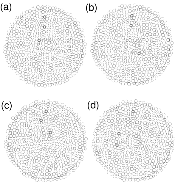
Figure 13: Snapshots from 2D systems undergoing Couette shear flow at $\phi=0.845$ and $b_{n}=0.0375$. Panels (b), (c), and (d) differ from panel (a) by $2$, $6$, and $19$ rotations, respectively. All particles with centers inside the inner ring at $r=R_{1}$ move at fixed rotation rate $\Omega=0.01$ counter clockwise. All particles with centers outside the outer ring at $r=R_{2}$ are stationary.

VI Future Directions

Several additional studies are necessary to fully understand dense shear flows in granular systems, and these will be presented in future work xu2 . First, we intend to investigate the influence of dynamic and static friction forces on the long-time stability of nonlinear velocity profiles. Preliminary results suggest that dynamic friction is not sufficient to stabilize nonlinear velocity profiles in systems undergoing planar shear flow. In initial studies with weak dissipation and dynamic friction remark3 near $\phi_{\rm rcp}$, we found that $t_{l}$ is similar to that for systems with dissipation and no dynamic friction. However, more extensive studies of dynamic as well as static friction are required to make a definitive statement about the influence of friction on the long-time stability of nonlinear velocity profiles aharonov ; volfson .

Figure 14: (a) Mean-square velocity fluctuations $\langle\delta v_{\theta}^{2}(r)\rangle$ in the tangential direction and (b) tangential velocity $v_{\theta}(r)$ normalized by the speed $v_{\theta}(R_{1})$ at the inner shearing boundary versus the distance from the inner boundary $(r-R_{1})/(R_{2}-R_{1})$ in a 2D Couette cell with $\phi=0.845$ and $b_{n}=0.0375$. The symbols indicate that time averages taken between the $20$th and $80$th (circles) or the $60$th and $80$th (triangles) rotations are nearly identical.

Second, most experimental studies of velocity profiles in granular systems are performed in (angular) Couette, not planar shear cells. How does the geometry of the shear cell influence the velocity profiles? Are shear bands stable in frictionless, athermal systems undergoing Couette shear flow? Fig. 13 shows preliminary results from studies of 2D Couette shear flow in systems at $\phi=0.845$, $b_{n}=0.0375$, and rotation rate $\Omega=0.01$ in the counter clockwise direction. Panels (b), (c), and (d) show snapshots of the system $2$, $6$, and $19$ rotations after the initial configuration in panel (a). The snapshots provided in panels (a) - (c) reveal that the shear band in this system is approximately $5-8$ small particle diameters wide since the two highlighted particles closest to the outer boundary do not rotate significantly even after $6$ rotations of the inner boundary. A comparison of panels (c) and (d) shows that at long times the particles in the flowing region are able to diffuse perpendicular to the boundaries. The mean-square velocity fluctuations $\langle\delta v_{\theta}^{2}\rangle$ in the tangential direction and the tangential velocity $v_{\theta}$ normalized by the speed at the inner boundary are shown in Figs. 14 (a) and (b) as a function of the distance from the inner boundary $(r-R_{1})/(R_{2}-R_{1})$. Averages over varied numbers of rotations demonstrate that the nonlinear velocity profiles are stable at long times. As we found in our studies of planar shear flow, nonlinear velocity profiles occur when the granular temperature is nonuniform. However, in Couette shear flows, the shear stress is also spatially dependent. Thus, the distinct contributions from nonuniform shear stress and nonuniform granular temperature need to be disentangled. In future work, we will determine whether nonlinear velocity profiles persist when we vibrate the outer boundary to create a more uniform granular temperature profile.

Finally, there have been several recent computational studies of effective temperatures defined from fluctuation dissipation relations, linear response theory, and elastic energy fluctuations in dense granular systems makse ; kondic ; ohernt . These studies have shown that a consistent effective temperature can be defined for dense shear flows, i.e. the effective temperatures $T_{\rm eff}$ obtained from the above definitions agree with each other but $T_{\rm eff}$ is much larger than the granular temperature of the system. Because $T_{\rm eff}$ describes fluctuations on long length and time scales, it is possible that the effective temperature will play a significant role in determining the shape of velocity profiles. Thus, it is important to study the effective temperature as well as the granular temperature in sheared glassy and athermal systems.

Acknowledgments

We thank J. Blawzdziewicz, A. Liu, and S. Nagel for helpful comments. Financial support from NSF DMR-0448838 (NX,CSO), NASA NNC04GA98G (LK), and the Kavli Institute for Theoretical Physics under NSF PHY99-07949 (CSO,LK) is gratefully acknowledged. We also thank Yale’s High Performance Computing Center for generous amounts of computing time.

References

- (1) D. Howell, R. P. Behringer, and C. Veje, Phys. Rev. Lett. 82, 5241 (1999); C. T. Veje, D. W. Howell, and R. P. Behringer, Phys. Rev. E 59, 739 (1999).
- (2) W. Losert, L. Bocquet, T. C. Lubensky, and J. P. Gollub, Phys. Rev. Lett. 85, 1428 (2000).
- (3) D. M. Mueth, Phys. Rev. E 67, 011304 (2003).
- (4) D. M. Mueth, G. F. Debregeas, G. S. Karczmar, P. J. Eng, S. R. Nagel, and H. M. Jaeger, Nature 406, 385 (2000).
- (5) N. W. Mueggenburg, Phys. Rev. E 71, 031301 (2005).
- (6) D. Fenistein and M. van Hecke, Nature 425, 256 (2003).
- (7) O. Pouliquen and R. Gutfraind, Phys. Rev. E, 552 (1996).
- (8) J. T. Jenkins, “Rapid granular shear flows driven by identical, bumpy frictionless boundaries,” in Powders and Grains 93, ed. C. Thornton (Balkema, Rotterdam, 1993).
- (9) R. D. Wildman, personal communication.
- (10) P. A. Thompson and G. S. Grest, Phys. Rev. Lett. 67, 1751 (1991).
- (11) E. Aharonov and D. Sparks, Phys. Rev. E 65, 051302 (2002).
- (12) D. Volfson, L. S. Tsimring, and I. S. Aranson, Phys. Rev. E 68, 021301 (2003); Phys. Rev. E 69, 031302 (2004).
- (13) F. da Cruz, S. Emam, M. Prochnow, J.-N. Roux, and F. Chevoir, cond-mat/0503682, (2005).
- (14) N. Xu, C. S. O’Hern, and L. Kondic, Phys. Rev. Lett. 94, 016001 (2005).
- (15) C. S. O’Hern, S. A. Langer, A. J. Liu, and S. R. Nagel, Phys. Rev. Lett. 88, 075507 (2002); C. S. O’Hern, L. E. Silbert, A. J. Liu, and S. R. Nagel, Phys. Rev. E 68, 011306 (2003).
- (16) W. H. Press, B. P. Flannery, S. A. Teukolsky, and W. T. Vetterling, Numerical Recipes in Fortran 77 (Cambridge University Press, New York, 1986).
- (17) H. J. Herrmann and S. Luding, Continuum Mech. Thermodyn. 10, 189 (1998).
- (18) F. Varnik, L. Bocquet, J.-L. Barrat, and L. Berthier, Phys. Rev. Lett. 90, 095702 (2003).
- (19) The transverse current correlation function is defined by , where . The dependence on frequency can be obtained by Fourier transforming .
- (20) J. P. Hansen and I. R. McDonald, Theory of Simple Liquids (Academic Press, London, 1986).
- (21) O. Baran and L. Kondic, Phys. Fluids (2005).
- (22) The glass transition temperature was calculated in equilibrium systems by measuring the density autocorrelation (at a wavenumber near the peak in the static structure factor) as a function of decreasing temperature. We made small temperature jumps and equilibrated the system at each temperature. We measured the structural relaxation time —the time at which decayed to —as a function of temperature and identified the glass transition temperature by fitting to a Vogel-Fulcher form vogel .
- (23) More precisely, the system is composed of large and small particles with diameter ratio , and thus we expect the largest granular temperature difference across the system to occur at frequencies near .
- (24) M. D. Ediger, C. A. Angell, and S. R. Nagel, J. Phys. Chem. 100, 13200 (1996)
- (25) N. Xu, C. S. O’Hern, and L. Kondic, (unpublished).
- (26) Granular systems with both dissipation and dynamic friction have nonconservative pair forces that are nonzero when two particles overlap , where . When , time evolution of the rotational degrees of freedom must also be considered.
- (27) H. A. Makse and J. Kurchan, Nature 415, 614 (2002).
- (28) L. Kondic and R. P. Behringer, Europhys. Lett. 67, 205 (2004).
- (29) C. S. O’Hern, A. J. Liu, and S. R. Nagel, Phys. Rev. Lett. 93, 165702 (2004).