Mixing properties of growing networks and the Simpson’s paradox

Abstract

We analyze the mixing properties of growing networks and find that, in some cases, the assortativity patterns are reversed once links’ direction is considered: the disassortative behavior observed in such networks is a spurious effect, and a careful analysis reveals genuine positive correlations. We prove our claim by analytical calculations and numerical simulations for two classes of models based on preferential attachment and fitness. Such counterintuitive phenomenon is a manifestation of the well known Simpson’s paradox. Results concerning mixing patterns may have important consequences, since they reflect on structural properties as resilience, epidemic spreading and synchronization. Our findings suggest that a more detailed analysis of real directed networks, such as the World Wide Web, is needed.

Complex networks arise in a wide range of interacting structures, including social, technological and biological systems NetReviews . Although all these networks share some generic statistical features, such as the small world property and the scale–invariance of the degree distribution, they also display differences and peculiarities when their structure is examined in detail.

A distinctive characteristic of a network is whether its nodes tend to connect to similar or unlike peers, the so–called mixing property newman02 . Similarity of nodes is established by comparing some node–dependent scalar quantity measuring a given quality. Borrowing terms from sociology, networks where properties of neighboring nodes are positively correlated are called assortative, while those showing negative correlations are called disassortative. Thus, assortative and disassortative mixing patterns indicate a generic tendency to connect respectively to similar or dissimilar pears. A scalar quantity naturally associated to each node in a network is its degree, measuring the number of neighboring nodes. The mixing by degree (MbD) is often measured by looking at how the average degree $K_{nn}$ of the nearest neighbors of a node depends on the degree $K$ of the node itself, and is a signature of correlations between other networks quantities fronczak05 . The mixing is assortative when $K_{nn}$ grows with $K$ and disassortative when it decreases pastor01 . The relevance of MbD lies in that, beyond discriminating among different network morphologies palla05 , it reflects important structural properties. Assortative networks are found to be more resilient against the removal of vertexes than disassortative ones vazquez03 . This implies, for example, that, when trying to block infection or opinion spreading within a social network hayashi04 ; blanchard05 , or to protect a computer network against cyber–attacks hayashi05 , different strategies are needed depending on the MbD properties of the underlying network. Moreover, it has recently been observed that the sign of degree correlations affect other properties of complex networks such as synchronization bernardo05 .

Recent studies show that social networks exhibit assortative MbD, whereas technological and biological ones display disassortative MbD newman03b . The Word Wide Web (WWW), a paradigmatic example of world–wide collaborative effort among millions of users and publishers, represents an anomaly: one would expect it to show assortative mixing, similarly to other social and collaborative networks, while it shows evidences of anticorrelations newman02 , and disassortative MbD capocci03 , which would rather put it in the realm of technological networks.

We aim to show that, in networks where a direction is naturally associated to the links, like in growing networks, it is crucial to distinguish between nearest neighbors along incoming and outgoing links. In the WWW case, for example, links with different direction have different roles and meanings: the outgoing links are drawn by individual web–masters, while they have no control on incoming links. In the language of Kleinberg kleinberg00 a page gains authority from incoming links, while it increases a peer’s authority by pointing to it. Nevertheless, the WWW has been often analyzed and modeled as an undirected network for what concerns its mixing properties capocci03 ; newman03c .

Our main result is that, in most cases, assortativity patterns are reversed when the direction of links in a network is taken into account: positive correlations among the degree of a node and the average degree of both upstream and downstream neighbors, considered separately, can disappear or even reverse when the different nature of neighboring sites is ignored and their degree are averaged together. Though this result may appear counterintuitive, the fact that pooling together data of different nature can generate spurious correlations is well known in the statistical literature, and often encountered in social sciences, medical statistics and finance, where, although it contains no logical contradiction, it is known as Simpson’s paradox simpson51 .

We show our result on two classes of complex growing networks: the linear preferential attachment (LPA) model dorogotsev00 , and the Bianconi–Barabasi (BB) fitness model bianconi01 . Both include as a special case the Barabasi–Albert (BA) model barabasi99 . In such growing network models, links have a natural direction – from newly added nodes to existing ones. Thus, in the following we distinguish between upstream and downstream neighbors, respectively along incoming and outgoing links.

To clarify our argument, we consider in detail the BA model (where calculations are simpler) before moving to the LPA and BB models. In the BA model, at each time step a node is added and attached to the network by $m$ undirected links with preferential attachment. A node $i$ (introduced at time $i$) points to existing nodes $j$ with probability $p_{j}(i)$ proportional to their degree $K_{j}(i)$ at time $i$ barabasi99 . Since $m$ sets a natural scale for the system, we will express all quantities in units of $m$, and denote them with the superscript $\sim$. On average, the degree of node $i$ grows in time as $\widetilde{K}_{i}(t)\simeq\sqrt{t/i}$ for $1\ll i\ll t$. The average degrees of neighbors of $i$, in $m$ units, read $\widetilde{K}_{nn,i}^{(in)}(t)=\sum_{j=i+1}^{t}\widetilde{K}_{j}(t)\widetilde{p}_{i}(j)/(\widetilde{K}_{i}(t)-1)$ and $\widetilde{K}_{nn,i}^{(out)}(t)=\sum_{j=1}^{i-1}\widetilde{K}_{j}(t)\widetilde{p}_{j}(i)$, where $\widetilde{K}_{nn,i}^{(in)}(t)$ and $\widetilde{K}_{nn,i}^{(out)}(t)$ refer to the degree of upstream and downstream neighbors respectively. By approximating the sum by an integral and the degree by its average, one gets $\widetilde{K}_{nn,i}^{(in)}(t)\simeq\log{\sqrt{t/i}}/(1-\sqrt{i/t})$ and $\widetilde{K}_{nn,i}^{(out)}(t)\simeq\sqrt{t/i}\log(A\sqrt{i})$, where $A$ is a constant of order one whose exact value depends on the initial condition nota1 . At a given time $t$, we can express the above quantities in terms of $\widetilde{K}$ and drop the $i$ dependence to get $\widetilde{K}_{nn}^{(in)}\simeq\widetilde{K}\log{\widetilde{K}}/(\widetilde{K}-1)$ and $\widetilde{K}_{nn}^{(out)}\simeq\widetilde{K}\log(\overline{K}/\widetilde{K})$, where $\overline{K}=A\sqrt{t}$ is of order of (and greater than) the maximum $\widetilde{K}$ observable at time $t$, which is $\widetilde{K}_{max}\simeq\sqrt{t}$. Thus $\widetilde{K}_{nn}^{(in)}$ is a monotonically (slowly) increasing function of $\widetilde{K}$, independent on $t$, and $\widetilde{K}_{nn}^{(out)}$ contains a $t$ dependence through $\overline{K}$ and for any $t$ is an increasing function of $\widetilde{K}$. We conclude that the degree of a node is positively correlated both with the average degree of upstream and downstream neighbors. However, computing the average degree of the neighbors altogether, correlations are lost and one gets $\widetilde{K}_{nn}(t)\simeq\log(A\sqrt{t})$, independent on $\widetilde{K}$ boguna03 . These results are confirmed by numerical simulation of the BA model and shown in Fig.1, where histograms of $\widetilde{K}_{nn}^{(in)}$, $\widetilde{K}_{nn}^{(out)}$, and $\widetilde{K}_{nn}$ are plotted as functions of $\widetilde{K}$ for $t=10^{4}$ and $m=100$, averaged over $10^{4}$ realizations.

Figure 1: Histogram of $\widetilde{K}_{nn}^{(in)}$ (squares), $\widetilde{K}_{nn}^{(out)}$(triangles), as functions of $\widetilde{K}$ from simulations of the the BA model, with $m=100$, $t=10^{4}$, and averaged over $10^{4}$ realizations.The behavior of $\widetilde{K}_{nn}$ is shown in the inset. The solid lines are the analytic calculations.

Let us now focus on the LPA model dorogotsev00 , a generalization of the BA model: according to the same dynamics, at the $i$–th time step $m$ directed links are drawn from $i$ to $j$ with probability $p_{j}(i)\propto k_{j}(i)+\alpha$, where $k_{j}(i)$ is the in–degree of site $j$ at time $i$. For $\alpha=m$, the BA model is recovered. When dealing with the LPA model, it is convenient to measure quantities in units $\alpha$. In the continuum time limit, the time dependence of the in–degree is $\widetilde{k}_{i}(t)=(t/i)^{\beta}-1$ with $\beta=(1+\alpha/m)^{-1}$. The degrees are power–law distributed with exponent $\gamma=2+\alpha/m$ dorogotsev00 . The calculation of the average in–degree of upstream and downstream neighbors can be performed in analogy to the BA model. The average degree of upstream neighbors reads $\widetilde{k}_{nn}^{(in)}\simeq(\widetilde{k}+1)\log(\widetilde{k}+1)/\widetilde{k}-1$, as in the BA model since it is independent from the ratio $\alpha/m$, and is monotonically increasing. The average degree of downstream neighbors is given by

$$\widetilde{k}_{nn}^{(out)}\simeq(1-\beta)(\widetilde{k}+1)\frac{\left(\frac{\bar{k}+1}{\widetilde{k}+1}\right)^{\frac{2\beta-1}{\beta}}-1}{2\beta-1}-1\,,$$ (1)

which is also an increasing function of the in–degree $\widetilde{k}$. $\widetilde{k}_{nn}^{(out)}$ contains an explicit dependence on $\alpha/m$ through $\beta$ and on $t$ through $\bar{k}$ ($\bar{k}\gtrsim\widetilde{k}_{max}\simeq t^{\beta}$). Note that now $\widetilde{k}_{nn}^{(in)}$ and $\widetilde{k}_{nn}^{(out)}$ count incoming links only. Instead, when ignoring the direction of links by averaging the degree over all nodes’ neighbors, one gets

$$\widetilde{k}_{nn}\simeq\frac{\widetilde{k}+1}{\widetilde{k}+\frac{\beta}{1-\beta}}\left(\log(\widetilde{k}+1)+\frac{\left(\frac{\bar{k}+1}{\widetilde{k}+1}\right)^{\frac{2\beta-1}{\beta}}-1}{2\beta-1}\right)-1\,.$$ (2)

Two different regimes appear, for $\alpha/m<1$ ($\beta>1/2$) and $\alpha/m>1$ ($\beta<1/2$), separated by $\alpha=m$ where the LPA model coincides with the BA model. The average in–degree of nearest neighbors increases as a function of $\widetilde{k}$ for $\beta<1/2$, while it decreases for $\beta>1/2$ barrat05 . The two regimes correspond to qualitatively different behaviors of the degree distribution: for $\alpha/m>1$ the distribution has finite variance in the thermodynamic limit($\gamma>3$), while $\alpha/m<1$ corresponds to $2<\gamma<3$, with diverging variance in the same limit. Summarizing, for the LPA model the degree of a node is positively correlated with the average degree of both upstream and downstream nearest neighbors. However, the average degree over all nearest neighbors increases or decreases for different values of the parameter $\beta$. A behavior similar to the $\beta>1/2$ case was already observed in simulations of a weighted directed model for the WWW barrat04 . In Fig 3 and 4 we show the results of our calculation, compared with simulation of the LPA model for $m=100$, $t=10^{4}$, and $\alpha=5$ for the $\beta>1/2$ regime (Fig. 3), and $m=100$, $t=10^{4}$, and $\alpha=500$ for the $\beta<1/2$ regime (Fig. 4).

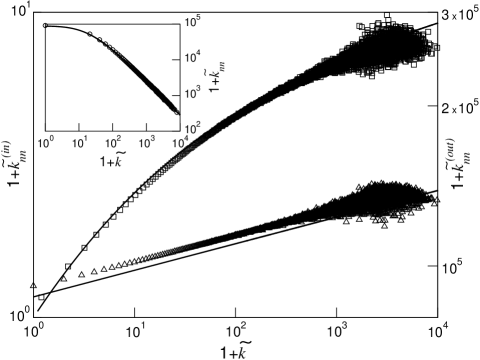
Figure 2: Histogram of $\widetilde{k}_{nn}^{(in)}$ (squares), $\widetilde{k}_{nn}^{(out)}$ (triangles), as functions of $\widetilde{k}$ for $t=10^{4}$, from simulations of the LPA model with $m=100$ and $\alpha=5$ ($\beta>1/2$), and averaged over $10^{4}$ realizations. The behavior of $\widetilde{k}_{nn}$ is shown in the inset. The solid lines are the analytic calculations.

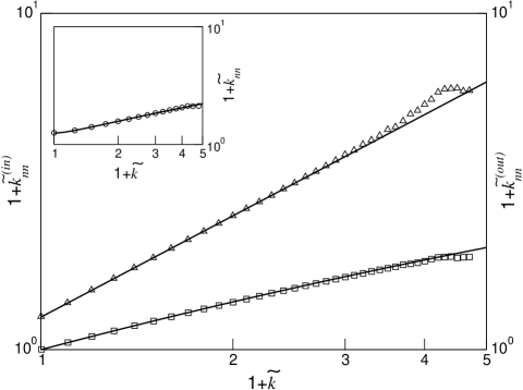
Figure 3: Histogram of $\widetilde{k}_{nn}^{(in)}$ (squares), $\widetilde{K}_{nn}^{(out)}$ (triangles), as functions of $\widetilde{k}$ for $t=10^{4}$, from simulations of the LPA model with $m=100$ and $\alpha=500$ ($\beta<1/2$), and averaged over $10^{4}$ realizations. The behavior of $\widetilde{k}_{nn}$ is shown in the inset. The solid lines are the analytic calculations.

Let now turn our attention to the BB model bianconi01 . The BB model was proposed as a realistic model for the WWW, and represents a paradigm for disassortatively mixed networks pastor01 . Here, the preferential attachment mechanism is modified to embody the intrinsic heterogeneity of nodes. This is done by assigning to each node $j$ a quenched random variable, or fitness, $\eta_{j}$. The network is grown by adding a node at each time step and connecting it to $m$ existing nodes chosen with probability proportional to both their degree and fitness $p_{j}(i+1)\propto\eta_{j}(k_{j}(i)+m)$. Now $k_{j}(i)$ depends on the single history of the network, and on the quenched variables $\left\{\eta_{l}\right\}_{l=1}^{i}$. However, for any given realization of the quenched disorder the degree can be approximated by $k_{j}(t)\simeq m\left((t/j)^{\eta_{j}/c}-1\right)$, where $c$ is a constant that depends on the probability distribution of the fitness bianconi01 . Thus, even though $k_{j}(t)$ is a function of all fitness, it essentially depends only on the value of the fitness at site $j$. This approximation is found to be very accurate numerically, and we will use it in what follows. Also, we approximate $p_{j}(t)$ by replacing the normalization factor $\sum_{l=1}^{i}\eta_{l}(k_{l}(i)+m)$ with its average value $mci$ barabasi99 . In the same notations as above, we will measure quantities in units of $m$. The average degree of downstream neighbors is given by $\widetilde{k}_{nn}^{out}(i)(t)=\sum_{j=1}^{i-1}\left\langle{\frac{\eta_{j}}{ci}\widetilde{k}_{j}(i)\widetilde{k}_{j}(t)}\right\rangle$; similarly the average degree of upstream neighbors is $\widetilde{k}_{nn}^{in}(i)(t,\eta_{i})=\frac{\eta_{i}}{c\widetilde{k}_{i}(t)}\sum_{j=i+1}^{t}\left\langle{\frac{\widetilde{k}_{i}(j)\widetilde{k}_{j}(t)}{j}}\right\rangle$, where brackets represent the average over $\eta_{j}$. Using the above approximations and computing the averages, one gets an expression for these quantities as functions of $i$ and $\eta_{i}$. The $\widetilde{k}$ dependence of $\tilde{k}_{nn}$ is then obtained by selecting couples $(i,\eta_{i})$ that give rise to a degree $\widetilde{k}$ after $t$ steps, which can be sampled numerically. The results for a uniform distribution of fitness in $[0,1]$ are shown in Fig. 4 where they are compared with results from direct simulations. Also in this case the degree of a node is positively correlated with the average degree of both upstream and downstream neighbors. However, as shown by Pastor–Satorras et al. pastor01 , the nearest neighbors average degree decreases as a function of the degree.

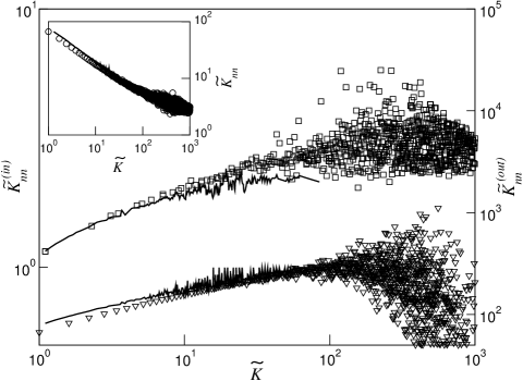
Figure 4: Histogram of $\widetilde{K}_{nn}^{(in)}=\widetilde{k}_{nn}^{(in)}+1$ (squares), $\widetilde{K}_{nn}^{(out)}=\widetilde{k}_{nn}^{(out)}+1$ (triangles), as functions of $\widetilde{K}=\widetilde{k}+1$ for $t=10^{4}$, from simulations of the BB model with $m=10$, and averaged over $10^{4}$ realizations. The behavior of $\widetilde{K}_{nn}=\widetilde{k}_{nn}+1$ is shown in the inset. The solid lines are histogram from integration of the analytic expression.

In summary, we have demonstrated the crucial role of link directions in the analysis of mixing patterns in complex networks, by showing that assortativity patterns are often reversed once a network is considered as directed. In the growing complex network models we have analyzed, we find positive correlations between the degree of a node and the average degrees of both upstream and downstream nodes, while fictitious correlations emerge when the different nature of the nodes is not taken into account. This is an example of the Simpson’s paradox that may occur any time data from different sources are pooled together. The correlation that appears in the pooled data is spurious: a positive correlation between two quantities before pooling results negative after pooling and vice versa. In the particular case of growing networks the degrees of upstream and downstream neighbors of a node are positive correlated with the degree of the node itself, however the correlation with upstream neighbors is much weaker. For increasing degrees, the fraction of weakly correlated neighbors increases. The overall neighbors’ average degree can then decrease as a result of the varied proportion, misleadingly suggesting the presence of negative correlations. In the case of BA networks, this effect exactly balances that of positive correlations.
Our findings suggest the need for more detailed analysis of real directed networks, such as the WWW, with a special focus on the direction of links between nodes. The counterintuitive properties described above may explain the anomalous exclusion of the WWW from the realm of social networks based on its observed disassortative mixing.

We thank Miguel–Angel Muñoz for useful discussions.

References

- (1) For recent reviews, see R. Albert and A.-L. Barabási Rev. Mod. Phys. 74, 47 (2002); M. E. J. Newman SIAM Review 45 167 (2003); S.N. Dorogovtsev and J.F.F. Mendes Evolution of Networks: From Biological Nets to the Internet and Www Oxford University Press (2003). R. Pastor-Satorras and A. Vespignani Evolution and Structure of the Internet : A Statistical Physics Approach Cambridge University Press (2004);
- (2) M. E. J. Newman Phys. Rev. E 67, 026126 (2003).
- (3) M. E. J. Newman Phys. Rev. Lett. 89, 208701 (2002).
- (4) A. Fronczak, P. Fronczak, cond–mat/0503069
- (5) R. Pastor–Satorras, A. Vázquez, and A. Vespignani Phys. Rev. Lett. 87, 258701 (2001).
- (6) G. Palla, I. Der nyi, I. Farkas, and T. Vicsek, Nature 435, 814 (2005).
- (7) A. Vázques and Y. Moreno Phys. Rev. E 67, 015101 (2003).
- (8) Y. Hayashi cond–mat/0408264.
- (9) Ph. Blanchard, A. Krueger, T. Krueger, and P. Martin, The Epidemic of Corruption physics/0505031.
- (10) Y. Hayashi and T. Miyazaki, cond–mat/0503615.
- (11) M. di Bernardo, F. Garofalo, and F. Sorrentino, cond–mat/0506236 (2005).
- (12) M. E. J. Newman and J. Park Phys. Rev. E 68, 036122 (2003).
- (13) A. Capocci G. Caldarelli, and P. De Los Rios Phys. Rev. E 68, 047101 (2003).
- (14) J. M. Kleinberg, in Proceedings of the 32nd Annual ACM Symposium on Theory of Computing.
- (15) Simpson, E.H., Journal of the Royal Statistical Society B 13, 238 (1951); Blyth, C. R., Journal of the American Statistical Association 67, 364 (1972).
- (16) The average over realizations of the degree of a node grows in time as , where . For large this gives the asymptotic . Each node appears at time with a degree equal to , so that . For it is convenient to choose , so that . The coefficient is sensibly different (value in the continuum time approximation) only for , for which , and we will approximate it with one for all other values, so that finally for , while . With this initial conditions . Analogous calculations can be performed for the LPA model, where is replaced by . This gives .
- (17) M. Boguñà and R. Pastor-Satorras, Physical Review E, 68, 036112 (2003).
- (18) S.N. Dorogovtsev, J.F.F. Mendes, and A.N. Samukhin, Phys. Rev. Lett. 85, 4633 (2000).
- (19) G. Bianconi and A.-L. Barabási Europhys. Lett., 54, 436 (2001).
- (20) A. L. Barabási and R. Albert, Science 286, 509 (1999).
- (21) G. Bianconi, G. Caldarelli, and A. Capocci, cond-mat/0408349.
- (22) M. Catanzaro, G. Caldarelli, and L. Pietronero, Physical Review E, 70, 037101 (2004).
- (23) J.J. Ramasco, S.N. Dorogovtsev, and R. Pastor-Satorras, cond-mat/0403438.
- (24) A. Barrat, R. Pastor-Satorras, Phys. Rev. E 71, 036127 (2005).
- (25) A. Barrat, M. Barthélemy, and A. Vespignani Lecture Notes in Computer Science 3243 56 (2004).