Implementation of the histogram method for equilibrium statistical models using moments of a distribution

Abstract

This paper shows a simple implementation of the Histogram Method for extrapolations in Monte Carlo simulations, using the moments of the operators that define the energy, instead of their histogram. This implementation is suitable for extrapolation over several operators, a type of calculation that is hindered by computer memory limitations. Examples of this approach are given for the 2-D Ising model.

I Introduction

The calculation of the expectation value of some operator $\Phi$ in a system in contact with a heath-bath of temperature $T$

$$\langle\Phi\rangle_{T}=\frac{\sum_{i}{\Phi_{i}\exp(-E_{i}/k_{B}T)}}{\sum_{i}{\exp(-E_{i}/k_{B}T)}},$$ (1)

is the usual task of equilibrium statistical mechanics. Here $E_{i}$ and $\Phi_{i}$ are, respectively, the energy and the value of $\Phi$ associated to the $i$-th configuration, and the sum runs over all possible configurations. These expectation values are usually impossible to calculate analytically, but there are many techniques to approximate expectation values in the canonical ensemble. Some of them are quite powerful and general, like high-temperature expansions and renormalization group techniques.

A different approach, quite successful in many applications, is the numerical simulation (“Monte Carlo Simulation”) of the ensemble metropolis1 ; newman-barkema ; landau-binder . This paper is concerned with the Histogram Method, introduced years ago to extrapolate the results of a Monte Carlo simulation conducted at a point in parameter space —for instance, some given temperature and magnetic field—, to a range of those parameters. It was formulated by by Ferrenberg and Swendsen ferrenberg1 ; ferrenberg2 , although there are some earlier proposals valleau1 . For completeness, a short description of this technique follows: Assume for instance that one has a model where the only control parameter is the temperature, and wants to compute the behavior of some function $f$ of the energy $E$. At some given $T$ one performs a Monte Carlo simulation using any given algorithm that generates $Q$ configurations with the correct probability, given by their Boltzmann weight, measures $f(E)$ for each configuration, and calculates finally the average value $\langle f(E)\rangle$. This average may be taken directly, or going through the preliminary construction of a normalized histogram $W_{T}(E)$ for the energies found in the simulation. One can write then

$$\langle f(E)\rangle_{T}\approx\frac{1}{Q}\sum_{q=1}^{Q}f(E_{q})=\sum_{E}{W_{T}(E)f(E)},$$ (2)

which is approximation to Eq. (1) with $\Phi=f(E)$. This equation can also written in terms of the density of states $g(E)$

$$\langle f(E)\rangle_{T}=\frac{\sum_{E}g(E)f(E)\exp(-E/(k_{B}T))}{\sum_{E}{g(E)\exp(-E/(k_{B}T))}}.$$ (3)

Comparing Eqs. (2) and (3) it is clear that $W_{T}(E)$ is proportional to $g(E)\exp(-E/(k_{B}T))$, and so an approximation for the density of states —ignoring normalization for the moment— is given by $g(E)\approx W_{T}(E)\exp(E/(k_{B}T))$. Notice that $g(E)$ is a property of the system itself, independent of temperature.

With an approximated density of states at hand the results of the simulation are extended to other temperatures. Eq. (3) written for a different temperature $T^{\prime}$ gives

$$\langle f(E)\rangle_{T^{\prime}} = \frac{\sum_{E}g(E)f(E)\exp(-E/(k_{B}T^{\prime}))}{\sum_{E}{g(E)\exp(-E/(k_{B}T^{\prime}))}}$$ (4)

$$\approx \frac{\sum_{E}W_{T}(E)f(E)\exp(E/(k_{B}T)-E/(k_{B}T^{\prime}))}{\sum_{E}{W_{T}(E)\exp(E/(k_{B}T)-E/(k_{B}T^{\prime}))}},$$

and one says that the histogram $W_{T}(E)$ has been reweighted.

II Expansion in Moments

In general, with the Histogram Method results obtained at a given point in the space of control parameters can be extrapolated to a neighborhood of that point. However, the implementation of the method can be cumbersome for models with more than one parameter, because the size of the histograms generated becomes too large. For instance, an Ising model in a simple cubic lattice, with nearest-neighbor, next-nearest-neighbor and magnetic couplings has a 3D parameter space. When applying the histogram method to this system one faces the problem of handling a histogram with a total number of bins that rapidly becomes impossible to accommodate in the computer’s physical memory. For instance, for a very modest size $L=16$, one needs to store some $16^{3}\approx 4\times 10^{3}$ possible values for each of the 3 couplings, and this gives a histogram with around $64\times 10^{9}$ bins. Working with 4 Byte integers (which may be insufficient for very large runs) gives a memory requirement around 250 GBytes, realizable in large workstations and supercomputers, but usually beyond the reach of the commodity machines used by many scientist today not-dense .

Among possible solutions one could coarse-grain the binning of the histogram (this is unavoidable if one is dealing with continuous variables, like in the XY or Heisenberg Models); one could also store a record of the operators of interest for all configurations generated by the Monte Carlo algorithm (this has been recommended for Hamiltonians with continuous variables newman-barkema ; ferrenberg3 ). Here I propose a different option that arises from two simple facts: one, most of the quantities one is interested in calculating can be expressed in terms of moments of the same operators that constitute the Hamiltonian. Two, the reweighting function can be easily expanded in a power series. Then, the physical quantities one wants to estimate at different values of the couplings can be obtained as power series in the increments of said couplings, using the moments of the operators obtained at some fixed point in parameter space as coefficients. A similar approach was proposed in Ref. rickman1 , using cumulants instead of moments; This approach via moments is bit simpler. Here I also show some details of implementation needed to insure larger ranges of numerical convergence.

To fix ideas, I shall use a simple example, namely, the Ising Model with zero magnetic field. The Hamiltonian is

$${\cal H}=-J\sum_{<a,b>}S_{a}S_{b}.$$ (5)

Assume now that one calculates the expectation value of some power of the magnetization, say $\langle M^{2}\rangle$, at some given temperature $T$. Define for convenience the adimensional energy operator $\Theta\equiv\sum_{<a,b>}S_{a}S_{b}$ and the couplings $K\equiv J/k_{B}T$. From Eq. (1) one gets

$$\langle M^{2}\rangle_{K}=\frac{\sum_{i}{M_{i}^{2}\exp(K\Theta_{i})}}{\sum_{i}{\exp(K\Theta_{i})}}.$$ (6)

Now, if one wants to calculate this same expectation value at some other temperature, one could store the histogram for $\Theta$ and then reweight it. But one can also write the desired expectation value

$$\langle M^{2}\rangle_{K^{\prime}}=\frac{\sum_{i}{M_{i}^{2}\exp(K^{\prime}\Theta_{i})}}{\sum_{i}{\exp(K^{\prime}\Theta_{i})}}=\frac{\sum_{i}{M_{i}^{2}\exp(K\Theta_{i})\exp((K^{\prime}-K)\Theta_{i})}}{\sum_{i}{\exp(K\Theta_{i})\exp((K^{\prime}-K)\Theta_{i})}},$$ (7)

and expand the exponential containing $K^{\prime}-K$ in a Taylor series

$$\langle M^{2}\rangle_{K^{\prime}}=\frac{\sum_{i}{M_{i}^{2}\exp(K\Theta_{i})\sum_{n=0}^{\infty}{(K^{\prime}-K)^{n}\Theta_{i}^{n}/n!}}}{\sum_{i}{\exp(K\Theta_{i})\sum_{n=0}^{\infty}{(K^{\prime}-K)^{n}\Theta_{i}^{n}/n!}}}.$$ (8)

For finite systems the order of the sums can be safely interchanged, giving

$$\langle M^{2}\rangle_{K^{\prime}}=\frac{\sum_{n=0}^{\infty}{[(K-K^{\prime})^{n}/n!]\sum_{i}{M_{i}^{2}\Theta_{i}^{n}\exp(K\Theta_{i})}}}{\sum_{n=0}^{\infty}{[(K-K^{\prime})^{n}/n!]\sum_{i}{\Theta_{i}^{n}\exp(K\Theta_{i})}}}.$$ (9)

One can now divide numerator and denominator by the partition function $Z(K)$ and find that the terms at the end of both expressions are the expectation values (moments, in short), of $M^{2}\Theta^{n}$ and $\Theta^{n}$, respectively, taken at $K$. Denoting $\delta K\equiv K-K^{\prime}$ one gets

$$\langle M^{2}\rangle_{K^{\prime}}=\frac{\sum_{n=0}^{\infty}{(\delta K)^{n}\langle M^{2}\Theta^{n}\rangle_{K}/n!}}{\sum_{n=0}^{\infty}{(\delta K)^{n}\langle\Theta^{n}\rangle_{K}/n!}}.$$ (10)

Since the expansion of the exponential function is convergent everywhere, there is no a priori limitation for this approach. But it is clear that one can never actually calculate all the required moments, and a truncation needs to be applied. This immediately introduces very strong bounds in the applicability of the method, since for large $\delta K$ the two sums in the previous expression require the inclusion of higher and higher moments if reasonable results are going to be obtained. A discussion about the number of moments needed to insure certain range of convergence is given later on.

Once the series are truncated, one faces a more serious difficulty: consider again the $M^{2}$ example, and assume that a simulation has been conducted in a lattice with $N$ spins. Since $M$ is an extensive quantity, $\langle M^{2}\rangle$ is of order $N^{2}$, and the range of $K$ where some degree of numerical convergence can be achieved is quite small. To find a way around this problem —at least partially—, begin by working with densities instead of with the original operators. Going back to our example, define $m\equiv M/N$ and $\theta\equiv\Theta/N$. The previous expression is rewritten as

$$\langle m^{2}\rangle_{K^{\prime}}=\frac{\sum_{n=0}^{\infty}{(N\delta K)^{n}\langle m^{2}\theta^{n}\rangle_{K}/n!}}{\sum_{n=0}^{\infty}{(N\delta K)^{n}\langle\theta^{n}\rangle_{K}/n!}}$$ (11)

Now it is clear that, since $\langle\theta\rangle$ is of order one, one may expect numerical convergence of the strongly truncated series up to

$$\Delta K\approx\frac{1}{N}\quad\rightarrow\quad\Delta T\approx\frac{T^{2}}{N},$$ (12)

which is a very narrow range; here ‘strongly truncated’ means a series with a few terms, say, less than 20. This is actually a very conservative bound, since the $n!$ in the denominators improve numerical convergence (and guarantees it for the infinite series).

The convergence of the truncated series can be improved if one notices that the desired moments are taken from a sharply peaked distribution. The combination of the fast increasing density of states $g(\Theta)$ and the fast decreasing Boltzmann weight implies the existence of a narrow distribution $W_{K}(\theta)$ —that is, the histogram in $\theta$—, centered in some value $\theta_{c}$. Going back now to Eq. (6), one may see that the zero values of the operators appearing in the energy (and therefore in the energy density) can be easily shifted. For instance, if one shifts the density $\theta$ by some value $\theta_{R}$, the expectation value for $m^{2}$ becomes

$$\langle m^{2}\rangle_{K}=\frac{\sum_{i}{m_{i}^{2}\exp(NK\theta_{i})}}{\sum_{i}{\exp(NK\theta_{i})}}=\frac{\sum_{i}{m_{i}^{2}\exp(NK(\theta_{i}-\theta_{R}))}}{\sum_{i}{\exp(NK(\theta_{i}-\theta_{R}))}},$$ (13)

since the factors of $\exp(-NK\theta_{R})$ cancel in the fraction. Now, if the value one chooses for $\theta_{R}$ is close to the center of the distribution, the moments one gets for $\delta\theta\equiv\theta-\theta_{R}$ are going to be numerically small —and become smaller the higher the moment and the larger the lattice—, simply because of the narrowness of the originating distribution. Retracing the steps taken going from Eqs. (7) to (10) one gets the final expression for $\langle m^{2}\rangle_{K^{\prime}}$ as

$$\langle m^{2}\rangle_{K^{\prime}}=\frac{\sum_{n=0}^{n^{*}}{(N\delta K)^{n}\langle m^{2}(\delta\theta)^{n}\rangle_{K}/n!}}{\sum_{n=0}^{n^{*}}{(N\delta K)^{n}\langle(\delta\theta)^{n}\rangle_{K}/n!}},$$ (14)

where both numerator and denominator series have been truncated to $n^{*}$ terms. Now the fast growth in the $N\delta K$ coefficients is partially balanced by a fast decrease in the values of $\langle(\delta\theta)^{n}\rangle_{K}$ and $\langle m^{2}(\delta\theta)^{n}\rangle_{K}$, and in this way the applicability of the method is extended to a much wider range in couplings. It is not too difficult to calculate the range of expected convergence of the extrapolation. In fact, for temperatures away from the critical point the width of $W_{K}(\theta)$ is order $1/\sqrt{N}$, from where one gets a range of convergence for the extrapolation of

$$\Delta K\approx\frac{1}{\sqrt{N}}\quad\rightarrow\quad\Delta T\approx\frac{T^{2}}{\sqrt{N}},$$ (15)

which comes from estimating $N\,\Delta K\,\Delta\theta\approx 1$. Close to the critical point the width of $W_{T}(\theta)$ increases, and scales as $\Delta\theta\approx N^{\alpha/(2\nu d)}/\sqrt{N}$. From here one estimates then a range of convergence

$$\Delta T\approx\frac{T^{2}}{\sqrt{N^{1+\alpha/(\nu d)}}}.$$ (16)

Here $\alpha$ and $\nu$ are the exponents for specific heath and correlation distance close to the critical point, and $d$ is the dimensionality. For a small $\alpha$ this is still a much wider range than the one gotten when no shifts are used. Notice that for the 2D Ising Model one replaces $N^{\alpha/(\nu d)}$ by $\ln N$ and gets an scaling

$$\Delta T\approx\frac{T^{2}}{\sqrt{N\ln N}}.$$ (17)

Notice finally that the example given here, that extrapolates for $m^{2}$, can be easily extended to any other lattice operator.

II.1 Example: the 2-D Ising Model: extrapolations at $h=0$

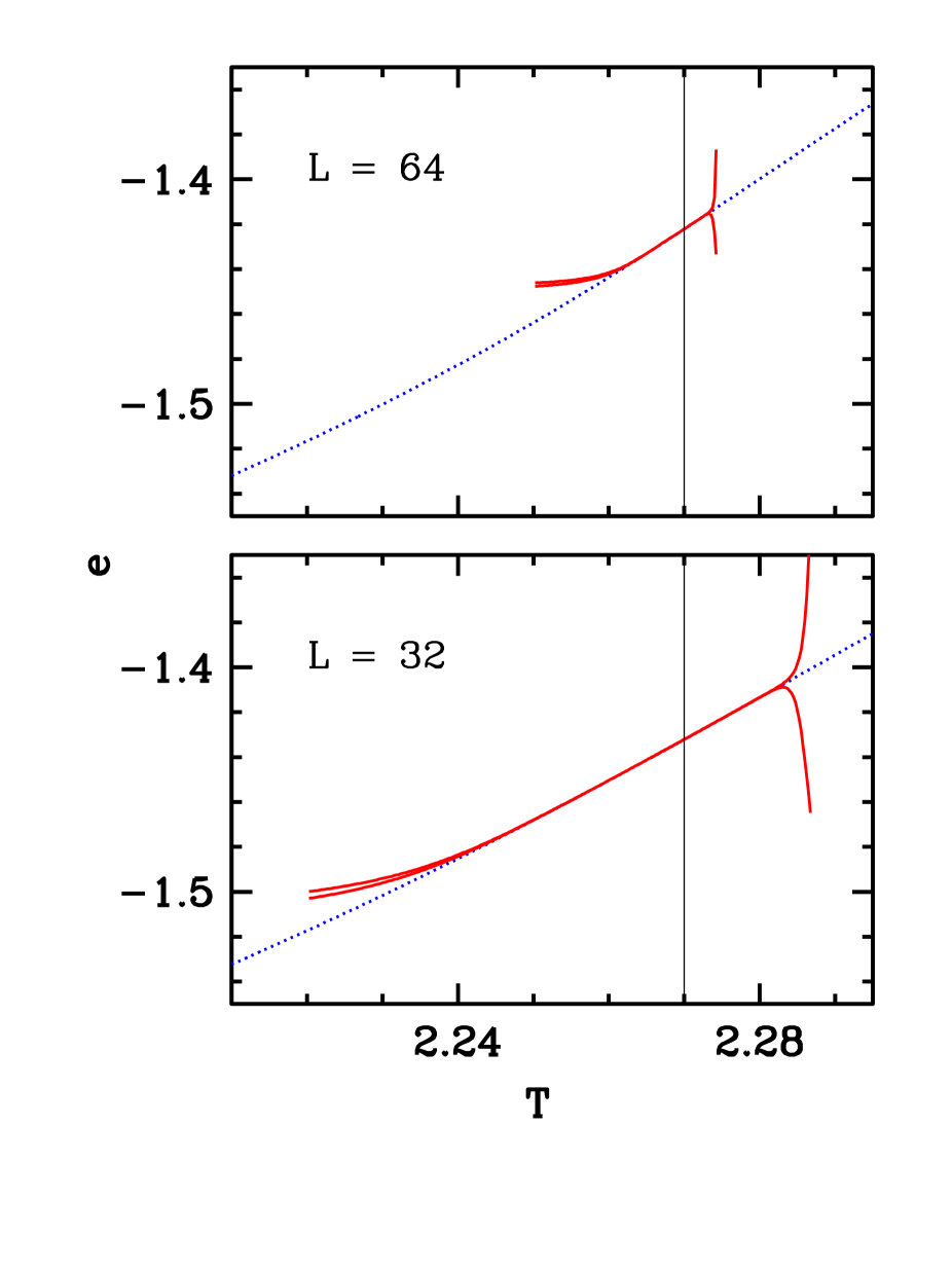
Figure 1: Energy per site vs. Temperature for the 2-D Ising Model, for $L=32$ and $L=64$. The dotted line gives the exact results obtained from the Kauffman solution. The solid lines give 14- and 15-moment extrapolations using values from a simulation at $T=2.27$ (indicated by the vertical line). Here the moments are taken without using any shifts ($\theta_{R}=0$).

A numerical test of the method was done for the two-dimensional Ising Model in square lattices of sizes 16, 32 and 64, with the Hamiltonian given in Eq. (5). Two Monte Carlo simulations were carried out using the Wolff algorithm wolf1 , at a temperature of $k_{B}T/J=2.27$, close to the critical temperature for the model. All moments of the form $\langle m^{l}(\delta\theta)^{n}\rangle$ and $\langle(\delta|m|)^{l}(\delta\theta)^{n}\rangle$ for $0\leq l,n\leq 16$ were recorded. First a short run with no shifts in either $\theta$ or $|m|$ was done, using $2\times 10^{6}$, $3\times 10^{6}$ and $4.4\times 10^{6}$ Wolff iterations for $L=16$, $32$ and $64$, respectively, after discarding transients of $120$, $170$ and $270$ iterations. The running time for this set of simulations was about $1,800$ seconds in a 2.4 GHz Pentium 4 processor. The exact solutions for the energy and the specific heath were obtained from the analytic free energy for finite lattices found by Kaufman kaufman1 . Fig. (1) shows the results of the extrapolation for the adimensional energy density $\langle\theta\rangle$ using either 14 or 15 moments numberofmoments , when no shift in $\theta$ has been implemented, compared with the exact results. It is clear that the range of applicability of the extrapolation is extremely narrow, as expected from Eq. (12). That estimate gives here $\Delta T_{32}=0.0050$ and $\Delta T_{64}=0.0013$. This estimate is quite conservative, and the figure gives ranges of numerical convergence which are 2 to 3 times longer.

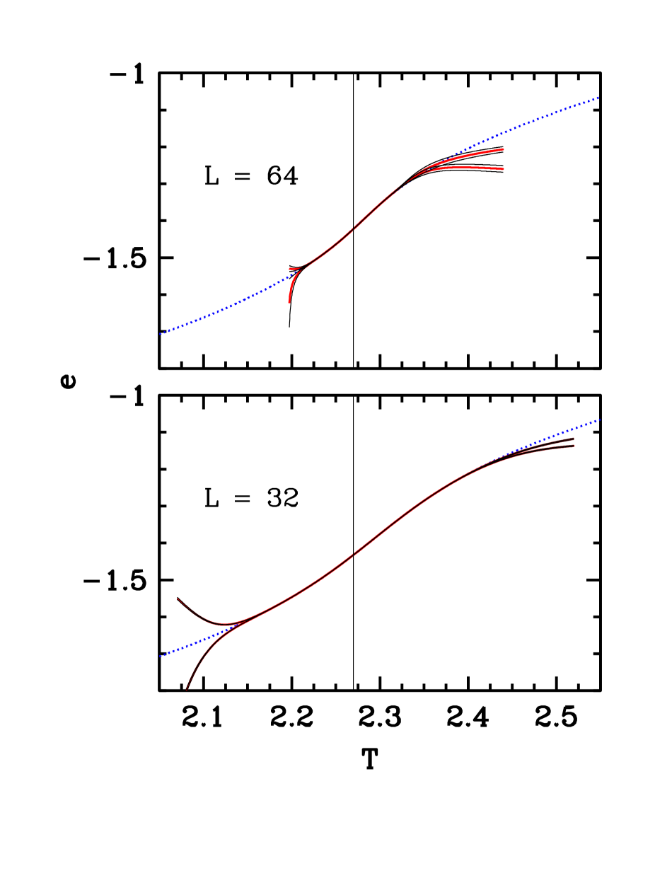
Figure 2: Energy per site vs. Temperature for the 2-D Ising Model, for $L=32$ and $L=32$. The dotted line gives the exact results obtained from the Kaufman solution. The thick solid lines give 14- and 15-moment extrapolations using values from a simulation at $T=2.27$ (indicated by the vertical line). The thin solid lines give the error bars for the extrapolations. Here the moments are taken using values of $\theta_{R}$ of $-1.432094$ for $L=32$ and $-1.422108$ for $L=64$.

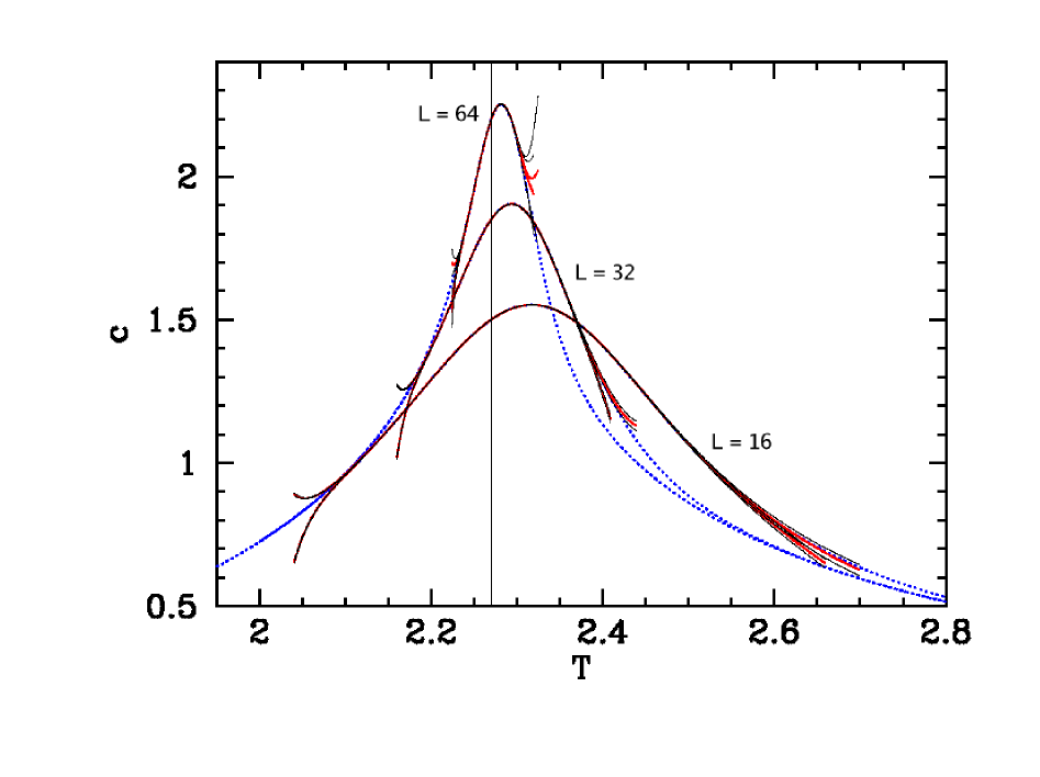
Figure 3: Specific heath per site vs. Temperature for the 2-D Ising Model, for $L=16$, $32$ and $64$. The dotted lines give the exact results obtained from the Kaufman solution. The thick solid lines give 13- and 14-moment extrapolations using values from a simulation at $T=2.27$ (indicated by the vertical line). The thin solid lines give the error bars for the extrapolations. Here the moments are taken using values of $\theta_{R}$ of $-1.451724$ for $L=16$, $-1.432094$ for $L=32$, and $-1.422108$ for $L=64$.

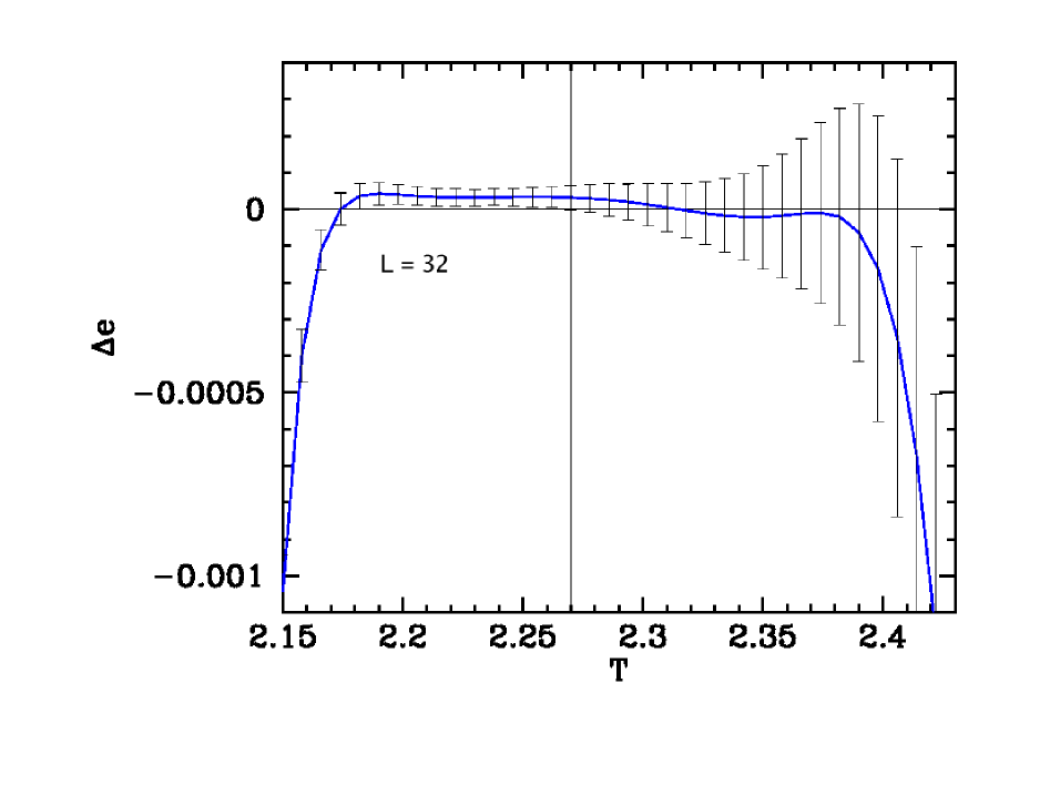
Figure 4: Error in the extrapolation of the energy density for $L=32$. The solid line gives the difference between the extrapolated energy and the exact Kaufman solution. The error bars correspond to the extrapolation. Here 15 moments were used. Here $\theta_{R}=-1.432094$.

The second simulation was a larger run where the results for $\langle\theta\rangle$ and $\langle|m|\rangle$ from the first were used as reference values $\theta_{R}$ and $|m|_{R}$ for the shifts. The total numbers of Wolff iterations were $4\times 10^{7}$, $6\times 10^{7}$ and $8.8\times 10^{7}$ for $L=16$, $32$ and $64$, respectively, after transients of $120$, $170$ and $250$ iterations were discarded. The total time for this set of simulations was about $37,000$ seconds with the same processor. Data were divided in 20 blocks in order to generate error estimates. Extrapolation for energy and specific heath were calculated. The results for the energies are given in Fig. (2), those for specific heath in Fig. (3), and in both figures a comparison with the exact results is given. It is clear that the range of applicability of the extrapolation is larger, and actually a bit larger than the estimation made in Eq. (17), which gives $\Delta T_{32}=0.061$ and $\Delta T_{64}=0.028$. Two important points should be remarked: First, for $\langle\theta\rangle$ the direction in which the extrapolated curves deviate from the correct results, for low $T$, depends on the number of moments taken into account; they deviate upwards when one uses 14 moments, and downwards when using 15 moments. A similar behavior is found for $c$, except that now the two extrapolations deviate in different directions at both ends of the range of convergence. This gives a very simple way of bounding the range of convergence of the algorithm. Second, the statistical errors in the extrapolations grow as one moves away from the simulated temperature, but the effect of this growth is smaller than the effect of the change in the number of included moments. The behavior of both types of errors are given in Fig. (4), which shows the difference between extrapolated and exact energies for $L=32$. The behavior for errors is similar for the specific heath. Notice that the statistical errors in the extrapolated results actually become smaller for temperatures a bit below the point where the simulation was carried out; this curious phenomenon has been studied in full histogram extrapolations ferrenberg3 .

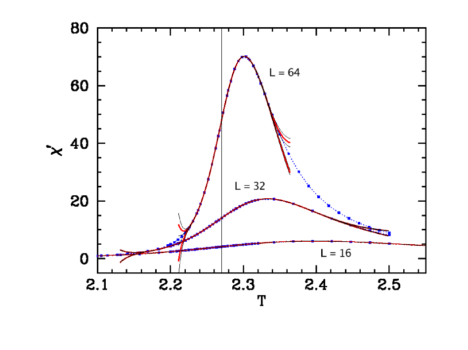
Figure 5: Susceptibility $\chi^{\prime}$, calculated using $|m|$, for the 2-D Ising model with $L=16$, $32$ and $64$. The points are from independent simulations, carried out at their nominal temperatures, an the dotted line is given only as a guide to the eye. The solid lines correspond to extrapolations from a simulation at $T=2.27$, using 15 and 16 moments.

The moments of $|m|$ were used to generate an extrapolated estimation of the susceptibility $\chi^{\prime}$, defined by $\chi^{\prime}=NK^{\prime}(\langle|m|^{2}\rangle-\langle|m|\rangle^{2})=NK^{\prime}(\langle m^{2}\rangle-\langle|m|\rangle^{2})$. This expression is used instead of the true susceptibility $\chi$ which in a numerical experiment does not give the expected peak close to the critical temperature ferrenberg4 . Fig. (5) shows a comparison between the extrapolated $\chi^{\prime}$ and values obtained in other individual simulations. These were obtained at their nominal temperatures using the Wolff algorithm. It is remarkable how the extrapolated results manage to reproduce reasonable well the peak in the susceptibility. Here one can also notice that the order of the approximation again decides in which direction the extrapolated results deviate form the actual values, and so a simple comparison between the 15- and 16-moments expansions gives bounds for the region of convergence of the method.

II.2 Example: the 2-D Ising Model with magnetic field

As mentioned before, this algorithm becomes attractive especially in cases where one has to deal with Hamiltonians composed of several operators, where the sizes of the histograms needed for reweighting may overflow the available memory. As a simple example consider again the 2-dimensional nearest-neighbor Ising Model, but now with a magnetic field. The Hamiltonian is

$${\cal H}=-J\sum_{<a,b>}S_{a}S_{b}-H\mu\sum_{a}S_{a},$$ (18)

giving a Boltzmann weight

$$\exp(-{\cal H}/k_{B}T))=\exp(K\Theta+hM),$$ (19)

where the additional definitions $M\equiv\sum_{a}S_{a}$ and $h\equiv H\mu/k_{B}T$ have been introduced. Consider now a simulation carried out at some temperature and magnetic field. Assuming that one wants to extrapolate the expectation value of some operator $\Phi$, one gets

$$\langle\Phi\rangle_{K^{\prime},h^{\prime}}=\frac{\sum_{i}\Phi_{i}\exp(K\Theta_{i}+hM_{i})\exp((K^{\prime}-K)\Theta_{i}+(h^{\prime}-h)M_{i})}{\sum_{i}\exp(K\Theta_{i}+hM_{i})\exp((K^{\prime}-K)\Theta_{i}+(h^{\prime}-h)M_{i})}.$$ (20)

As before, it is better to change all operators into their densities, defining $m\equiv M/N$ and $\phi\equiv\Phi/N$. Also, the density $\theta$ should be shifted so that its distribution is centered close to zero (this is unnecessary for $m$, since its distribution is symmetric around $m=0$). Performing these operations and the Taylor expansions for the exponential containing $\delta K$ and $\delta h$, one gets, repeating the same steps that gave Eq. (14), the following expression

$$\langle\phi\rangle_{K^{\prime}h^{\prime}}=\frac{\sum_{l=0}^{\infty}\sum_{n=0}^{\infty}(N\delta K)^{l}(N\delta h)^{n}\langle\phi(\delta\theta)^{l}m^{n}\rangle_{K,h}/(l!n!)}{\sum_{l=0}^{\infty}\sum_{n=0}^{\infty}(N\delta K)^{l}(N\delta h)^{n}\langle(\delta\theta)^{l}m^{n}\rangle_{K,h}/(l!n!)}.$$ (21)

One should pay attention here to the fact that for low temperatures the histogram $W_{K,h}(\theta,m)$ becomes bimodal in $m$, and the assumption of a distribution with a single narrow peak is no longer valid. However, close to the critical point the width in $m$ of such histogram remains small, and one can still get by with the first few moments. Occasionally, it may be convenient to work in terms of $|m|$, whose distribution remains unimodal.

The data obtained from the previous simulations were now used to generate the behavior of the magnetization and the susceptibility at non-zero values of $H$. For the magnetization one gets, after truncation

$$\langle m\rangle_{K^{\prime}h^{\prime}}=\frac{\sum_{l=0}^{l^{*}}\sum_{n=0}^{n^{*}}(N\delta K)^{l}(Nh)^{n}\langle(\delta\theta)^{l}m^{n+1}\rangle_{K,h=0}/(l!n!)}{\sum_{l=0}^{l^{*}}\sum_{n=0}^{n^{*}}(N\delta K)^{l}(Nh)^{n}\langle(\delta\theta)^{l}m^{n}\rangle_{K,h=0}/(l!n!)};$$ (22)

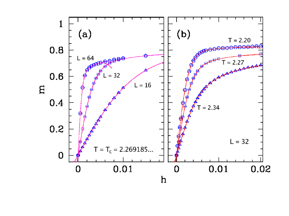
Figure 6: Magnetization vs. $H$ for the 2-D Ising model. The lines give the values extrapolated from a simulation at $T=2.27$, $H=0$, and the points, with their error bars, correspond to individual simulations carried out at their nominal $T$ and $H$ values. (a): Results for $T=T_{c}=2.269185\ldots$, with sizes $L=16$ (triangles), $32$ (squares) and $64$ (round marks). The split visible for the $L=64$ line correspond to the separation between the 14- and the 15-moments extrapolations. (b) Results for $L=32$, with temperatures $T=2.34$ (triangles), $T=2.27$ (squares) and $T=2.20$ (round marks). In both cases the extrapolated statistical errors come out smaller than the thickness of the lines.

an analogous expression is obtained for $\langle m^{2}\rangle_{K^{\prime},h^{\prime}}$, and from here the true susceptibility can be computed. The results are shown in Fig. (6), which shows: (a) magnetization vs. $H$ for $L=16$, $32$ and $64$ at the critical temperature $T_{c}=2/\ln(1+\sqrt{2})=2.269185...$, and (b) magnetization vs. $H$ for $L=32$ at $T=2.20$, $2.27$ and $2.34$. In all cases the magnetization has been extrapolated from the simulations that were carried out at $H=0$ and $T=2.27$. In a slight departure from what was done before, here the denominator in Eq. (22) was calculated using 16 moments while the sums in the numerator were truncated to $15$ or $14$ moments. The individual points have been calculated using a modified version of the Wolff algorithm, were the acceptance ratio depends on the change of energy due to a cluster flipping in the presence a magnetic field $H$. It is clear from the figure that the expansion in moments reproduces quite well the behavior of the magnetization for each temperature and lattice size, and in particular it manages to show the large growth of $m$ with $H$ as $T$ is reduced. The splits in the extrapolation curves correspond to the separation of the $15$- and $14$-moment extrapolations, and mark the end of the ranges of convergence. For small lattices these splits do not appear in the $H$ range tested here.

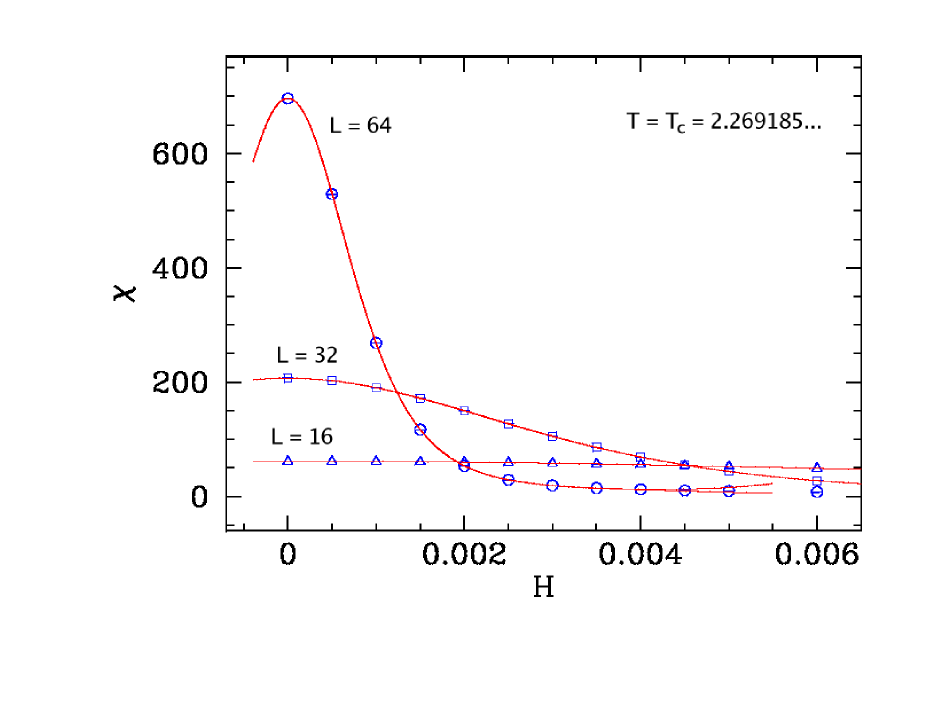
Figure 7: True susceptibility $\chi$ vs. $H$ for the 2-D Ising model. The lines give the values extrapolated from a simulation at $T=2.27$, $H=0$, and the points, with their error bars, correspond to individual simulations carried out at their nominal $T$ and $H$ values. Results shown here are for $T=T_{c}=2.269185\ldots$, with sizes $L=16$ (triangles), $32$ (squares) and $64$ (round marks). The split visible for the $L=64$ line correspond to the separation between the 14- and the 15-moments extrapolations. The extrapolated statistical errors come out smaller than the thickness of the lines.

Finally, Figs. (7) and (8) show the true susceptibility $\chi$ as a function of $H$, for $T=T_{c}$ and $L=16$, $32$ and $64$, and for $L=32$ and $T=2.20$, $2.27$ and $2.34$. It should be noticed that the extrapolation manages to cover quite well the whole peak in $\chi$. The results for $L=32$ and different temperatures also show an excellent agreement between extrapolations and individual simulations, and show how the method can really extrapolate in more than one parameter. Notice that, as expected, $\chi$ grows as $T$ is reduced, even below $T_{c}$; for $H=0$ the true susceptibility is just proportional to $\langle m^{2}\rangle$. Otherwise, the behavior the extrapolated quantities vis a vis the individual simulations at $H\neq 0$ is in all respects analogous the results found before: a very good correspondence for small $H$ —that is, close to where the simulation was carried out—, followed by a large deviation, which depends on the number of moments included in the extrapolation.

III Conclusions

This paper shows how to implement the histogram method for extrapolation of results of a Monte Carlo simulation using the moments of the histogram. This approach has several advantages over the direct method —histogram construction and posterior reweighting—, and over the method of storing configurations for their reweighting (named “histogram on the fly” in Ref. ferrenberg3 ). To start with, the resulting expressions for the extrapolated quantities are given by very simple and conceptually appealing formulas. Second, the ranges of applicability of the method become evident simply by changing the number of moments included in the extrapolation. Third, the amount of computer memory and physical storage needed are so small that one may without any problem generate several repetitions of the simulations so as to generate in a simple way the error estimates for the extrapolated quantities. And finally, this approach eliminates completely the need to choose a binning size in cases of continuous variables.

One needs however to balance these benefits against the cost of the extra approximation involved in the method. After all, replacing a full histogram for its first few moments necessarily reduces precision. How many moments one really needs to keep in any given simulation so that not too much information is lost is an issue that has to be considered with some care. On the one hand, it is clear that increasing too much the number of stored moments not only defeats one of the motivations for this approach, which is to work with a limited memory, but also necessarily runs into the limits of reliability imposed by the statistical errors of the simulation. On the other, not keeping enough moments implies a waste of simulation time. As a first approach to the answer to this question one can consider the following estimation, done here for a one-coupling Hamiltonian: consider the preliminary run needed for the estimation of $\theta_{c}$. This preliminary run can also be used to obtain a rough estimate of the width $\sigma_{\theta}$ of the distribution. Now, the order of magnitude of the moments $\langle(\delta\theta)^{n}\rangle$ will be around $\sigma_{\theta}^{n}$, and so the terms needed in an estimation with a shifted coupling look like (see Eq. (14))

$$\frac{(\Delta K)^{n}\langle(\delta\theta)^{n}\rangle}{n!}\approx\left(\frac{e\Delta K\sigma_{\theta}}{n}\right)^{n}.$$ (23)

It is not difficult to show, using a steepest descent approximation, that as a function of $n$ this expression behaves as a Gaussian centered in $n_{\max}=\Delta K\,\sigma_{\theta}$, with a width given by $\sqrt{n_{\max}}$ and height $\exp(n_{\max})$. Therefore one gets

$$\frac{(\Delta K)^{n}\langle(\delta\theta)^{n}\rangle}{n!}\approx\exp(\Delta K\sigma_{\theta})\,\exp\left(\frac{(n-\Delta K\sigma_{\theta})^{2}}{2\Delta K\sigma_{\theta}}\right).$$ (24)

The conclusion is then the following: given an initial estimation of the width $\sigma_{\theta}$ of the distribution, and assuming that a certain maximum extrapolation range $\Delta K$ is going to be used, the main contribution to the extrapolation comes from the moments with $n$ around $n_{\max}=\Delta K\sigma_{\theta}$. Besides, one finds that the moments with $n$ such that $n-n_{\max}\gg\sqrt{n_{\max}}$ are basically irrelevant. The numerical results shown here display a much larger dependence on the number of moments used than on the statistical spread of the data, suggesting that several more moments may have been used in the extrapolation before reaching the limits given by statistical spread.

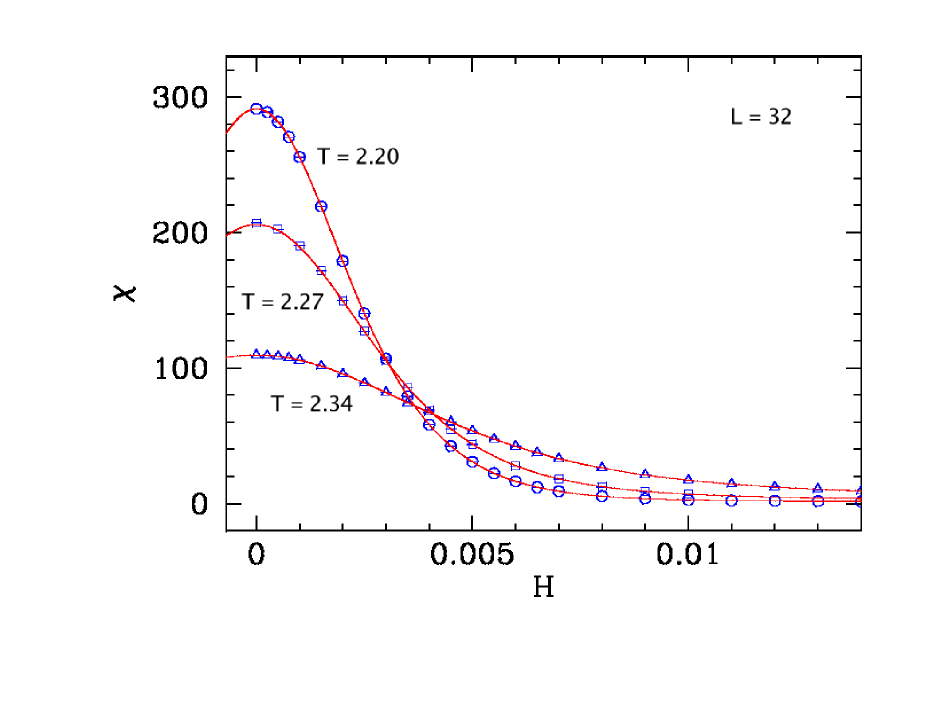
Figure 8: True susceptibility $\chi$ vs. $H$ for the 2-D Ising model. The lines give the values extrapolated from a simulation at $T=2.27$, $H=0$, and the points, with their error bars, correspond to individual simulations carried out at their nominal $T$ and $H$ values. Results shown here are for $L=32$, with temperatures $T=2.34$ (triangles), $T=2.27$ (squares) and $T=2.20$ (round marks). The extrapolated statistical errors come out smaller than the thickness of the lines.

References

- (1) Electronic address: gperez@mda.cinvestav.mx
- (2) N. Metropolis, A. W. Rosenbluth, N. M. Rosenbluth, A. M. Teller and E. Teller, J. Chem. Phys. 21, 1087 (1953).
- (3) See, e.g., M. E. J. Newman and G. T. Barkema, Monte Carlo Methods in Statistical Physics, Oxford U. P. (Oxford, 1999).
- (4) See, e.g., D. P. Landau and K. Binder, A Guide to Monte Carlo Simulations in Statistical Physics, Cambridge U. P. (Cambridge, 2000)
- (5) A. M. Ferrenberg and R. H. Swendsen, Phys. Rev. Lett. 61, 2635 (1988); Phys. Rev. Lett. 63, E1658 (1989).
- (6) A. M. Ferrenberg and R. H. Swendsen, Phys. Rev. Lett. 63, 1195 (1989).
- (7) A large list of works in the Histogram Method that predate the papers of Ferrenberg and Swendsen is given in Ref. [18] of J. Lee and J. M. Kosterlitz, Phys. Rev. B 43, 3265 (1991).
- (8) It may be argued that there is no need for such a large array to be stored, since in practice many bins will never get hit because the corresponding combination of values for the three operators (nearest-neighbor, next-nearest-neighbor and magnetic) is not allowed. This observation is correct, but in general it may be quite difficult to know beforehand which combinations of lattice operators are allowed and which are not, or even how many are allowed. It is then not possible to request the correct amount of computer memory at the start of a simulation. A possible solution is to request new memory locations only when needed, but then one is never sure about the maximum lattice size that can be safely explored.
- (9) A. M. Ferrenberg, D. P. Landau and R. H. Swendsen, Phys. Rev. E 51, 5092 (1995).
- (10) J. M. Rickman and S. R. Phillpot, Phys. Rev. Lett. 66, 349 (1991).
- (11) U. Wolff, Phys. Rev. Lett. 62, 361 (1989).
- (12) B. Kaufman, Phys. Rev. 76, 1232 (1949).
- (13) Since the numerator in the extrapolation of contains moments of the form , one can run up to when moments are kept. For simplicity, the same bound is used for the denominator. Similarly, for the extrapolation of one can run up to when moments are kept.
- (14) A. M. Ferrenberg and D. P. Landau, Phys. Rev. B 44, 5081 (1991).