Cell Dynamics Simulation of Kolmogorov-Johnson-Mehl-Avrami Kinetics of Phase Transformation

Abstract

In this study, we use the cell dynamics method to test the validity of the Kormogorov-Johnson-Mehl-Avrami (KJMA) theory of phase transformation. This cell dynamics method is similar to the well-known phase-field model, but it is a more simple and efficient numerical method for studying various scenarios of phase transformation in a unified manner. We find that the cell dynamics method reproduces the time evolution of the volume fraction of the transformed phase predicted by the KJMA theory. Specifically, the cell dynamics simulation reproduces a double-logarithmic linear KJMA plot and confirms the integral Avrami exponents $n$ predicted from the KJMA theory. Our study clearly demonstrates that the cell dynamics approach is not only useful for studying the pattern formation but also for simulating the most basic properties of phase transformation.

1 Introduction

Phase transformation occurs by the nucleation and subsequent growth of a nucleus in a system where the first-order phase transformation takes place. It has attracted much attention for more than a half century [1, 2, 3, 4, 5] from a fundamental point of view as well as from technological interests. These include the mechanical properties of metallic materials [6], the recrystallization of deformed metals [7], and the manufacturing of basic thin-film transistor devices, such as solar cells and active matrix-addressed flat-panel displays [8].

The nucleation and growth processes are often described in terms of the old standard theory called the KJMA theory developed by Kolmogorov [1], Johnson and Mehl [2], and Avrami [3, 4, 5]. According to this theory, the time evolution of the volume fraction of a new transformed phase follows the linear KJMA plot with the integral Avrami exponent $n$ that is given by the slope. However, it is recognized that this theory often fails to explain experimental results [9, 10]; neither the KJMA plot becomes linear nor the Avrami exponent becomes an integer. There is also some debate about the validity of the assumption used in the theory [11]. To resolve the discrepancy, a realistic yet efficient simulation method that could take various factors into account is indispensable.

The direct atomic-scale computer simulation of the kinetics of phase transformation using the molecular dynamics or Monte Carlo method is still a difficult task. Even the most fundamental phenomenon, such as nucleation, is not easy to study using these methods. Instead, the problem of phase transformation has been tackled using a coarse-grained Ginzburg-Landau-type model called the Cahn-Hilliard [12], Ginzburg-Landau [13] or phase-field [14, 15] model, which requires the solution of highly nonlinear partial differential equations. Since this model requires the time integration of the partial differential equations, it is not easy to simulate the long-time behavior of the dynamics of phase transformation [16] except for special traveling wave solutions [17, 18].

A model based on a cellular automaton instead of a partial differential equation can improve the efficiency of numerical integration [19, 6]. It has been used to test the KJMA theory in the recrystallization of metals. Although the cellular automaton is sufficiently flexible to implement the various local reactions of recrystallization, it does not have a direct connection to the equilibrium phase diagram. Therefore, the connection between the phase diagram and the phase transformation is not so clear compared to the Ginzburg-Landau-type model mentioned above.

In this study, instead, we use the cell dynamics method [20, 21] to study the validity of the KJMA theory. This method is attractive because it has the merit of cellular automata and is computationally efficient, and yet it keeps the connection to the phase diagram through the Landau-type free energy. The format of this paper is as follows: in §2, we review the cell dynamics method and present the necessary modification for studying the nucleation and growth. In §3, we follow closely the work by Jou and Lusk [14] and test the validity of the KJMA theory using the cell dynamics method. We conclude in section 4.

2 Cell Dynamics Method for Nucleation and Growth

To study the phase transformation, it is customary to study the partial differential equation called the phase-field model [14, 15] which is equivalent to the time-dependent Ginzburg-Landau (TDGL) [13] or Cahn-Hilliard model [12]:

$$\frac{\partial\psi}{\partial t}=-\frac{\delta\cal F}{\delta\psi},$$ (1)

where $\delta$ denotes the functional differentiation, $\psi$ is the nonconserved order parameter, and $\cal F$ is the free energy functional. This free energy is usually written as the square-gradient form

$${\cal F}[\psi]=\frac{1}{2}\int\left[D(\nabla\psi)^{2}+h(\psi)\right]{\rm d}{\bf r}.$$ (2)

The local part $h(\psi)$ of the free energy $\cal F$ determines the bulk phase diagram and the value of the order parameter in equilibrium phases. The double-well form was frequently used for $h(\psi)$ to express the two-phase coexistence and study the phase transformation between these two phases.

This TDGL equation (1) for the nonconserved order parameter $\psi$ was loosely transformed into a space-time discrete cell dynamics equation by Puri and Oono [21] following a similar transformation of the kinetic equation for the conserved order parameter called the Cahn-Hilliard-Cook equation [20]. In their cell dynamics method, the partial differential equation (1) is replaced by a finite difference equation in space and time in the form

$$\psi(t+1,n)=F[\psi(t,n)],$$ (3)

where the time $t$ is discrete and an integer, and the space is also discrete and is expressed by the integral site index $n$. The mapping $F$ is given by

$$F[\psi(t,n)]=-f(\psi(t,n))+\left[\ll\psi(t,n)\gg-\psi(t,n)\right],$$ (4)

where $f(\psi)=dh(\psi)/d\psi$, and the definition of $\ll\cdots\gg$ for a two-dimensional square grid is given by [20, 21, 22]

$$\ll\psi(t,n)\gg=\frac{1}{6}\sum_{i=\mbox{nn}}\psi(t,i)+\frac{1}{12}\sum_{i=\mbox{nnn}}\psi(t,i),$$ (5)

where “nn” denotes nearest neighbors and “nnn” next-nearest neighbors. An improved form of this mapping for a three-dimensional case was also obtained [22].

Oono and Puri [20, 21] further approximated the derivative of the local free energy $f(\psi)$ called the “map function” in the $\tanh$ form

$$f(\psi)=\frac{dh}{d\psi}\simeq\psi-A\tanh\psi,$$ (6)

with $A=1.3$ that corresponds to the free energy [23]

$$h(\psi)=-A\ln\left(\cosh\psi\right)+\frac{1}{2}\psi^{2}$$ (7)

and is the lowest order ($O(\psi^{2})$) approximation to the double well form of the free energy

$$h(\psi)=-\frac{1}{2}\psi^{2}+\frac{1}{4}\psi^{4}$$ (8)

when $A=1.5$. They [20, 21] used this simplification since this cell dynamics system is invented not to simulate the mathematical TDGL partial differential equation but to simulate and describe the behavior of nature directly. Later, Chakrabarti and Brown [23] discussed that this simplification is justified since the detailed form of the double-well potential $h(\psi)$ is irrelevant to the long-time dynamics and the scaling exponent.

Subsequently, however, several authors used the map function $f(\psi)$ directly obtained from the free energy $h(\psi)$ as it is [24, 25] and found that the cell dynamics equation (3) is still tractable numerically. Ren and Hamley [25] argued that one can easily include the effect of the asymmetry of the free energy and the asymmetric characteristic of two phases using the original form of the free energy function $f(\psi)$.

Despite the popularity of this cell dynamics method in the soft-condensed matter community as a simulator of pattern formation due to various factors, it has not yet been used to study the most fundamental problem of phase transformation by nucleation and growth. In the next section, we use a parameterized free energy function, study the kinetics of phase transformation, and test the validity of the KJMA theory.

3 Numerical Results

3.1 Two-dimensional growth of single domain

To simulate the growing stable phase after the nucleation, we have to prepare the system in a state where one phase is metastable and has the higher free energy than the other stable phase. The free energy difference between the stable and metastable phases is determined from the supersaturation in liquid condensation and from the undercooling in crystal nucleation. Microscopically, this free energy difference is necessary for the nucleus to overcome the additional curvature effect caused by the interfacial tension and to continue to grow [26].

To study the growth of the stable phase using the cell dynamics method, we consider the time-dependent Ginzburg-Landau (TDGL) equation (1) with the square gradient free energy functional (2). The local part of the free energy $h(\psi)$ we used is [14]

$$h(\psi)=\frac{1}{4}\eta\psi^{2}(1-\psi)^{2}+\frac{3}{2}\epsilon\left(\frac{\psi^{3}}{3}-\frac{\psi^{2}}{2}\right).$$ (9)

This free energy is shown in Fig. 1, where one phase at $\psi=0$ is metastable while another phase at $\psi=1$ is stable. The free energy difference $\Delta h$ between the stable phase at $\psi=1$ and the metastable phase at $\psi=0$ is solely determined from the parameter $\epsilon$:

$$\Delta h=h(\psi=0)-h(\psi=1)=\frac{\epsilon}{4}.$$ (10)

Therefore, $\epsilon$ represents the supersaturation or the undercooling.

The metastable phase at $\psi=0$ becomes unstable when $\eta=3\epsilon$, which defines the spinodal. The height $\Delta E$ of the free energy barrier at $\psi=(\eta-3\epsilon)/2\eta$ can be tuned by the parameters $\eta$ and $\epsilon$:

$$\Delta E=h\left(\psi=\frac{\eta-3\epsilon}{2\eta}\right)-h(\psi=0)=\frac{\eta^{4}-4\eta^{3}\epsilon+27\epsilon^{4}}{32\eta^{3}},$$ (11)

which vanishes when $\eta=3\epsilon$ at the spinodal.

Figure 1: Model double-well free energy (9) that can realize two-phase coexistence when $\epsilon=0$. The parameter $\epsilon$ determines the free energy difference $\Delta h$, and the parameters $\eta$ and $\epsilon$ determine the free energy barrier $\Delta E$.

The steady-state analytical solution of the TDGL with a constant interfacial velocity has been obtained in one dimension by Chan [17] when the free energy $h(\psi)$ is written in the quadratic form such as in eq. (9). Using Chan’s formula, the interfacial velocity $v$ of our TDGL model (1), (2) with the free energy (9) is given by

$$v=\sqrt{\frac{D}{2\eta}}3\epsilon=\sqrt{\frac{D}{2\eta}}12\Delta h.$$ (12)

Chan [17] further suggested that if the interfacial width is small, the interfacial velocity of a two-dimensional circular or three-dimensional spherical growing nucleus is asymptotically given by eq. (12) of the one-dimensional model. The larger the free energy difference $\epsilon$ and the lower the free energy barrier $\eta$ are, the higher the front velocity $v$ becomes.

The critical radius $R_{c}$ of a two-dimensional circular nucleus is also given analytically [17, 14]:

$$R_{c}=\frac{D}{v}=\frac{\sqrt{2\eta D}}{3\epsilon}.$$ (13)

In the metastable phase, the circular nucleus of the stable phase with a radius ($R$) smaller than $R_{c}$ shrinks, while that with a radius larger than $R_{c}$ grows and its front velocity approaches eq. (12). Again, the larger the free energy difference $\epsilon$ and the lower the free energy barrier $\eta$ are, the smaller the critical radius $R_{c}$ is.

We implemented the above free energy (9) into the cell dynamics code written by Mathematica TM [27] for the animation of spinodal decomposition developed by Gaylord and Nishidate [28], and simulated the growth of a single circular nucleus of a stable phase.

Initially, we prepared a small circular nucleus of a stable phase within a metastable phase and simulated the growth of that nucleus. The system size is 100$\times$100 cells, $D$ in eq. (2) is $D=0.5$, and the periodic boundary condition is imposed. The initial order parameter $\psi$ is randomly chosen from $0.9\leq\psi\leq 1.1$ for the circular nucleus of the stable phase and from $-0.1\leq\psi\leq 0.1$ for the metastable environment. The diameter of the initial nucleus is fixed at $d=11$. Therefore, the initial nucleus occupies a part of 11$\times$11 cells. The effective area of the stable phase is computed by counting the number of cells with the order parameter $\psi>1/2$.

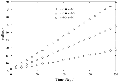
Figure 2: Evolution of effective radius of area of stable phase plotted as a function of time when $\eta=1$ and $\epsilon=0.1$ (open circles), $\eta=1.0$ and $\epsilon=0.3$ (open triangles), and $\eta=0.3$ and $\epsilon=0.1$ (open diamonds). The effective radius shows a linear time dependence, indicating a constant interfacial velocity.

Figure 2 shows the effective radius of the circular nucleus of the stable phase calculated from the effective area of the nucleus as a function of time step $t$. The nearly linear growth of the nucleus of the stable phase is clearly visible, which indicates a constant front velocity for the stable-metastable interface predicted from the analytical solution for the TDGL [17]. The velocities $v$ estimated from Fig. 2 and predicted from eq. (12) are compared in Table  1 together with the critical radius $R_{c}$ calculated from eq. (13). It can be seen that eq. (12) correctly predicts the general trend of the front velocity $v$ when the two parameters $\eta$ and $\epsilon$ are altered. Since the cell dynamics method does not solve the TDGL directly, the discrepancy between cell dynamics simulation and theoretical prediction (12) by a factor of roughly 2 is not very significant.

Table 1: Comparison of front velocities $v$ estimated by cell dynamics simulation and prediction using eq. (12) for various potential parameters $\eta$ and $\epsilon$. The corresponding critical radii $R_{c}$ are also tabulated.

$\eta$	1	1	0.7	0.5	0.4	0.3
$\epsilon$	0.1	0.3	0.1	0.1	0.1	0.1
$v$ (simulation)	0.063	0.22	0.082	0.10	0.12	0.14
$v$ [eq. (12)]	0.15	0.45	0.18	0.21	0.24	0.27
$R_{c}$ [eq. (13)]	3.3	1.1	2.8	2.4	2.1	1.8

From the above comparison of the values estimated by cell dynamics simulation and theoretical prediction using the steady-state solution of the TDGL for a two-phase system, we consider that this cell dynamics method is effective for studying the phase transformation by the growth of the multiple nucleus of the stable phase.

3.2 KJMA kinetics by cell dynamics simulation

3.2.1 Site-saturation nucleation

In site-saturation nucleation, a fixed number of nuclei are prepared initially, and subsequent growth is monitored. The KJMA theory gives an analytical expression for the volume fraction $f$ of the stable phase as a function of time $t$. In two dimensions, the formula leads to [14]

$$f=1-\exp\left(-\pi n_{0}v^{2}\left(t+t_{0}\right)^{2}\right),$$ (14)

where $n_{0}$ is the number density (number per unit area) of the randomly distributed initial nuclei. $v$ is the growth rate of the radius of each nucleus discussed in the previous section. $t_{0}$ is the origin of time which can hopefully take the incubation time of nucleation into account [15].

From eq. (14), we have

$$\log\left(-\ln(1-f)\right)=2\log\left(t+t_{0}\right)+\mbox{constant}.$$ (15)

Therefore, the KJMA theory predicts that a double logarithms $\log\left(-\ln(1-f)\right)$ versus $\log\left(t+t_{0}\right)$ is a straight line that is known as the KJMA plot with the integral tangent $n=2$, which is called the “Avrami exponent”.

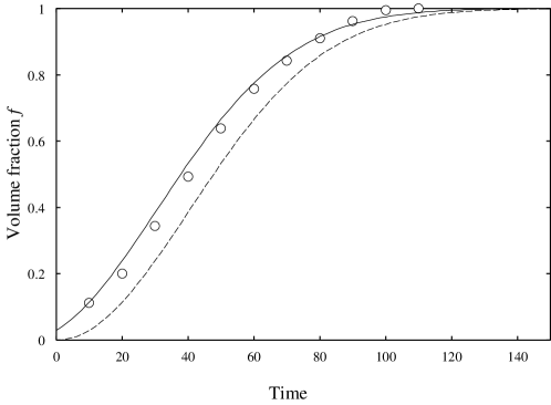
Figure 3: Evolution of volume fraction $f$ calculated by cell dynamics simulation for site-saturation nucleation as a function of time (open circles) when $\eta=1.0$ and $\epsilon=0.3$. The broken line denotes the theoretical prediction (14) with $t_{0}=0$, while the solid line denotes that with $t_{0}=10$. A better agreement between the simulation and theoretical results is attained when the incubation time $t_{0}=10$ is taken into account.

We have simulated the site-saturation nucleation using the cell dynamics method. Now a finite number of nuclei of the stable phase is distributed over the area we considered. The initial nuclei are circular and have the diameter $d=8$, which is larger than the critical radius $R_{c}$ in Table  1. Then, the evolution of the transformed volume is monitored as a function of time. Again, we have considered the 100$\times$100 system and introduced a finite number ($N_{0}=20$) of nuclei as the initial condition. Therefore, the number density of the initial nucleus is $n_{0}=20/10000=0.002$.

The time evolution of the transformed volume $f$ is plotted as a function of time $t$ in Fig. 3. When the effect of the incubation time with $t_{0}=10$ is included, a better agreement between the simulation and theoretical results is attained. This incubation time $t_{0}=10$ is the time necessary for a infinitely small nucleus to become a larger nucleus with the diameter $d=8$ in our simulation, and is estimated by fitting the theoretical curve (14) to the simulation data. Since an infinitely small nucleus cannot grow because it is smaller than the critical nucleus, we use the terminology “incubation time” to indicate both the time necessary for a critial nucleus to appear and the time necessary for it to grow to be a larger nucleus.

The KJMA plot of the double logarithm of the volume fraction $f$ is shown as a function of $\log t$ in Fig. 4, where we ignore the effect of the incubation time and set $t_{0}=0$. The time evolutions for several combinations of the potential parameters $\eta$ and $\epsilon$ are shown. They do not fit the expected straight lines.

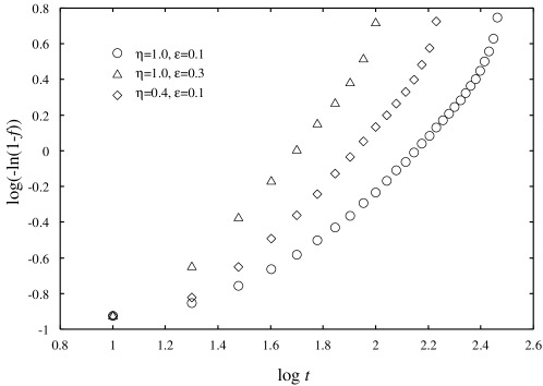
Figure 4: Evolution of volume fraction $f$ calculated by cell dynamics simulation for site-saturation nucleation as a function of time when $t_{0}=0$. The double logarithm $\log\left(-\ln(1-f)\right)$ is plotted as a function of the logarithm of time $\log t$. All data do not fit the straight lines predicted from the KJMA theory (15).

Figure 5 shows the KJMA plot when the incubation time $t_{0}$ is considered. Again, the incubation time $t_{0}$ is estimated by fitting the theoretical curve (14) to the simulation data. Now, the time evolutions for several combinations of the potential parameters $\eta$ and $\epsilon$ all fit the straight lines with almost the same Avrami exponent $n\simeq 2$, which is very close to the theoretical prediction, as shown in Table  2. The results in Figs. 4 and 5 clearly suggest that the incubation time $t_{0}$ should be carefully taken into account to deduce the Avrami exponent $n$ when we analyze experimental as well as simulation data.

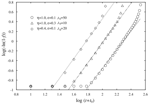
Figure 5: Same as Fig. 4 when incubation time $t_{0}$ is taken into consideration. All data follows an almost straight line and confirm the prediction of the KJMA theory given by eq. (15) with all the Avrami exponents $n$ deduced from the straight lines in the figure being close to the theoretically predicted $n=2$.

Table 2: Avrami exponent $n$ for site-saturation nucleation estimated by cell dynamics simulation for various potential parameters $\eta$ and $\epsilon$. The value theoretically predicted from the KJMA theory is $n=2$.

$\eta$	1	1	0.4
$\epsilon$	0.1	0.3	0.1
$n$ (simulation)	1.92	2.04	2.03

Figure 6 shows the evolution of the morphology of the two-dimensional system for the site-saturation nucleation when $\eta=0.4$ and $\epsilon=0.1$. We observe the almost isotropic growth of every nucleus of the stable phase. At the time step $\sim$100, almost all cells are transformed into the stable phase.

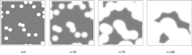
Figure 6: Typical evolution pattern of site-saturation nucleation calculated by cell dynamics simulation when $\eta=0.4$ and $\epsilon=0.1$. The white area indicates the stable phase.

3.2.2 Continuous nucleation

In the continuous nucleation, a new nuclear embryo is continuously introduced. The KJMA theory of continuous nucleation gives the analytical expression for the volume fraction $f$ of the growing stable phase. In two dimensions, it leads to [14]

$$f=1-\exp\left(-\frac{\pi\dot{n}v^{2}}{3}\left(t+t_{0}\right)^{3}\right),$$ (16)

where $\dot{n}$ is the steady nucleation rate per unit area and $v$ is the growth rate of the single nucleus discussed in the previous section.

From eq. (16), we have

$$\log\left(-\ln(1-f)\right)=3\log\left(t+t_{0}\right)+\mbox{constant}.$$ (17)

Therefore, a double logarithmic KJMA plot should give the “Avrami exponent” $n=3$ instead of $n=2$ of the site-saturation nucleation.

We have also simulated the continuous nucleation using the cell dynamics method. In our simulation, a constant nucleation rate $\dot{n}$ is achieved by introducing a new nucleus every $1/\dot{n}$ time step (nucleation time). At each nucleation time step, a position within the two-dimensional area is randomly selected. If the position is already occupied by the stable phase, no new nucleus is placed. If the position is not occupied by the stable phase, a new nucleus is placed and allowed to grow there. In this simulation, we have used a larger 200$\times$200 system to avoid the finite-size effect as much as possible. The steady nucleation rate $\dot{n}=0.1/40000$ is used. Therefore, a single nucleus is produced at every 10 time steps in the area 200$\times$200.

The time evolution of the transformed volume $f$ is plotted as a function of time $t$ in Fig. 7 as the double logarithmic KJMA plot. The time evolutions for several combinations of the potential parameters $\eta$ and $\epsilon$ show almost the same straight line with the Avrami exponent very close to the theoretically predicted $n=3$, as shown in Table  3.

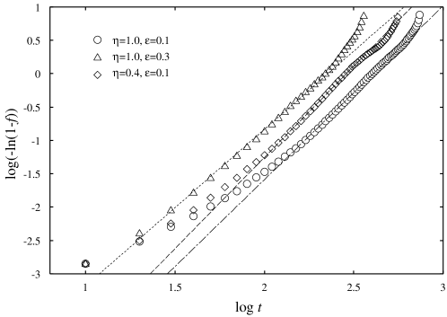
Figure 7: Evolution of volume fraction $f$ calculated by cell dynamics simulation for continuous nucleation as a function of time. The double logarithmic KJMA plot is used. All curves fit the straight lines predicted from the KJMA theory (17). The Avrami exponents deduced from the straight lines in the figure are all close to the theoretically predicted $n=3$, as summarized in Table  3.

Table 3: Avrami exponent $n$ for continuous nucleation estimated by cell dynamics simulation for various potential parameters $\eta$ and $\epsilon$. The value theoretically predicted from the KJMA theory is $n=3$.

$\eta$	1.0	1.0	0.4
$\epsilon$	0.3	0.1	0.1
$n$ (simulation)	2.35	2.60	2.73

Figure 8 shows the evolution of the morphology of the two-dimensional systems for the continuous nucleation when $\eta=0.4$ and $\epsilon=0.1$. Because a nucleus is continuously produced, almost all cells are occupied at the later stage, and then the production of a nucleus stops. The situation becomes closer to the site-saturation nucleation. The Avrami exponent $n$ smaller than the theoretically predicted $n=3$ for the continuous nucleation but closer to the site saturation nucleation $n=2$ is expected. This finite-size effect is one of the reasons why the Avrami exponent estimated from the simulation data in Table  3 is always smaller than the theoretically predicted $n=3$.

There is also a problem of incubation time in continuous nucleation. In our simulation, we have introduced a fairly large nucleus, which is sufficiently large to grow continuously. Thus, the same problem of time origin or incubation time $t_{0}$ as that for the site-saturation nucleation could occur. Since a nucleus is continuously produced, we could not incorporate the effect of incubation time in a reasonable manner in our analysis.

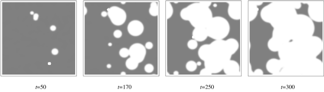
Figure 8: Typical evolution pattern of continuous nucleation simulation when $\eta=0.4$ and $\epsilon=0.1$.

In continuous nucleation, we found that the KJMA theory correctly describes the overall behavior of the time dependence of the transformed volume fraction $f$. However, there is a small inflection in the slope of the KJMA plot at around $\log(-\ln(1-f))\approx 0.0$, which can be explained by the impingement in which the growing circular grains collide with each other. The volume fraction $f$ when the impingement starts to occur is roughly estimated to be $f=\pi r^{2}/4r^{2}\approx 0.79$ using the ratio of the area of a circular grain with the radius $r$ to that of a square with the side length $2r$. Thus, the inflection of the KJMA straight line is expected at

$$\log(-\ln(1-f))=\log(-\ln(0.21))\approx 0.19,$$ (18)

which is very close to the point where the inflection is actually observed in Fig. 7. The same effect was discussed by Jou and Lusk [14]. The other factors affecting the Avrami exponent are discussed in the next subsection.

3.3 Discussion

Experimentally, a reasonably linear KJMA behavior was observed in the recrystallization of some metals and in the crystallization of metallic glasses [9]. However, a considerable variation in Avrami exponent $n$ defined by

$$\log\left(-\ln(1-f)\right)=n\log\left(t+t_{0}\right)+\mbox{constant}$$ (19)

was observed from the electrical resistivity and differential scanning calorimetry (DSC) data.

Following the argument of Christian [29], Price [9] proposed a formula for the Avrami exponent

$$n=a+b(1-q),$$ (20)

where $a$ is the nucleation component; $a=0$ for the site saturation and $a=1$ for the continuous nucleation. $b$ defines the dimensionality of the growth ($b=3$ for a three-dimensional problem and $b=2$ for our two-dimensional problem). The exponent $q$ includes contributions from various types of power-law reaction.

For example, in our cell dynamics model based on the Landau-type free energy (9), the driving force of phase transformation comes from the undercooling defined by eq. (10) that leads to the linear time-dependent growth of a circular nucleus with the constant front velocity $v$ given by eq. (12). However, as more materials are transformed into the stable phase, the driving force decreases somehow and the front velocity $v$ is expected to decelerate from eq. (12). Thus, it is reasonable to assume a power-law decay of the front velocity

$$v\propto t^{-q},$$ (21)

which exactly gives eq. (20). Hence, the Avrami exponent becomes smaller than the KJMA predicted $n=a+b$, as observed in our numerical simulations for the continuous nucleation.

There are many other factors affecting the exponent $n$. Possible reasons for the nonideal exponent and even the nonlinear growth in the KJMA plot include the nonrandomness of the nucleation site and the preferential nucleation, for example, at the grain boundary [30], the effect of the time dependence of the nucleation rate and so forth. The net result of these effects is a negative deviation from the KJMA linear plot [9], which leads to again the smaller exponent $n$ in accordance to the many experimental results and our simulation. In our cell dynamics method, these effects can be easily included by changing the probability of selecting the nucleation rate from cell to cell. Hesselbarth and Göbel [19] have included such effects in their cellular automaton and could successfully explain the deviation of experimental data from KJMA predicted data.

There is also a problem of two-stage crystallization [9, 31]. In some alloys, the KJMA plot shows an inflection in which the exponent $n$ changes markedly from a large value at an early stage to a small value at a later stage. However, our simulation data shown in Fig. 7 shows the opposite trend; the exponent $n$ is large at the later stage. This phenomena is explained by assuming that the early stage corresponds to the continuous nucleation and that the later stage corresponds to the site saturation because of the exhaustion of the nucleation site [31]. Recent theoretical model calculation supports this two-stage nucleation model [32, 33].

Our cell dynamics method could easily incorporate such a two-stage transformation by assuming that the continuous nucleation terminates at a certain stage. Then, the growth process is continuous nucleation with the exponent $n=3$ in the early stage, but it becomes site saturation with the exponent $n=2$ in the later stage. In our cell dynamics method, it is not necessary to assume a discrete lattice [32, 33] and is easier to incorporate various modifications to KJMA kinetics. Using our cell dynamics method, a more quantitative study is feasible in the future.

4 Conclusion

In this study, we used a cell dynamics method to test the validity of the Kolmogorov-Johnson-Mehl-Avrami (KJMA) kinetic theory of phase transformation. First, we used this method to study the growth of a single circular nucleus and found that the nucleus grows with a constant front velocity in accordance to the analytical solution [17]. Next, we used the cell dynamics method to simulate the growth of an ensemble of nuclei under the conditions of both the site saturation and continuous nucleation. We found a nearly linear behavior of the KJMA plot with the Avrami exponent close to the KJMA predicted value. Finally, we suggested several extensions of the cell dynamics method to study various contributions that may lead to the nonlinear KJMA behavior or nonideal Avrami exponent.

The results obtained in this study are summarized as follows:

• The cell dynamics method with a realistic free energy can succesfully simulate the steady growth of a single nucleus and confirm the prediction of Chan [17] based on the time-dependent Ginzburg-Landau (TDGL) equation.

• It can also simulate the growth of multiple nuclei and confirm the time evolution of the volume fraction of the transformed material predicted from the KJMA kinetic theory [1] and numerical simulation using TDGL [14].

• Therefore, the cell dynamics method can be used to simulate more complex scenarios of nucleation and growth.

• Our simulation indicates that the incubation time should be carefully taken into account when we deduce the Avrami exponent from the experimental and simulation data.

The cell dynamics method is similar to the time-dependent Ginzbug-Landau or Cahn-Hilliard model based on the free energy functional. In contrast to the conventional cellular automaton approach to the phase transformation [19, 6, 32, 33], no phenomenological energy that induces phase transformation is necessary. Therefore, the cell dynamics method is numerically efficient as a cellular automaton, yet it keeps the direct connection to the equilibrium phase diagram. This cell dynamics method can be used to test various scenarios of nucleation and growth in a unified manner.

References

- [1] A. N. Kolmogorov: Izv. Akad. Nauk SSSR, Ser. Mat. 3 (1937) 355.
- [2] W. A. Johnson and R. F. Mehl: Trans. AIME 135 (1939) 416.
- [3] M. Avrami: J. Chem. Phys. 7 (1939) 1103.
- [4] M. Avrami: J. Chem. Phys. 8(1940) 212.
- [5] M. Avrami: J. Chem. Phys. 9 (1941) 177.
- [6] V. Marx, F. R. Reher and G. Gottstein: Acta Mater. 47 (1999) 1219.
- [7] R. D. Doherty: Prog. Mater. Sci. 42 (1997) 39.
- [8] Y. Uemoto, E. Fujii, A. Nakamura, K. Senda and H. Takagi: IEEE Trans. Electron Devices 39 (1992) 2359.
- [9] C. W. Price: Acta Metall. Mater. 38 (1990) 727.
- [10] V. Erukhimovitch and J. Baram: Phys. Rev. B 51 (1995) 6221.
- [11] C. DeW. Van Siclen: Phys. Rev. B 54 (1996) 11845.
- [12] J. W. Cahn and J. E. Hilliard: J. Chem. Phys. 31 (1959) 688.
- [13] O. T. Valls and G. F. Mazenko: Phys. Rev. B 42 (1990) 6614.
- [14] H.-J. Jou and M. T. Lusk: Phys. Rev. B 55 (1997) 8114.
- [15] M. Castro: Phys.Rev. B 67 (2003) 035412.
- [16] T. M. Rogers, K. R. Elder and R. C. Desai: Phys. Rev. B 37 (1988) 9638.
- [17] S.-K. Chan: J. Chem. Phys. 67 (1977) 5755.
- [18] M. Iwamatsu and K. Horii: Phys. Lett. A 214 (1996) 71.
- [19] H. W. Hesselbarth and I. R. Göbel: Acta Metall. Mater. 39 (1991) 2135.
- [20] Y. Oono and S. Puri: Phys. Rev. A 38 (1988) 434.
- [21] S. Puri and Y. Oono: Phys. Rev. A 38 (1988) 1542.
- [22] P. I. C. Teixeira and B. M. Mulder: Phys. Rev. E 55 (1997) 3789.
- [23] A. Chakrabarti and G. Brown: Phys. Rev. A 46 (1992) 981.
- [24] S. Qi and Z.-G. Wang: Phys. Rev. Lett. 76 (1996) 1679.
- [25] S. R. Ren and I. W. Hamley: Macromolecules 34 (2001) 116.
- [26] M. Iwamatsu: J. Phys.: Condens. Matter 5 (1993) 7537.
- [27] S. Wolfram: The Mathematica Book, 5th ed. (Wolfram Media, Champaign IL, 2003).
- [28] R. J. Gaylord and K. Nishidate: Modeling Nature: Cellular Automata Simulation with Mathematica (Springer, Heidelberg, 1996).
- [29] J. W. Christian: The Theory of Transformations in Metals and Alloys (Pergamon Press, Oxford, 1965).
- [30] J. W. Cahn: Acta Metall. 4 (1956) 449.
- [31] J. J. Burton and R. P. Ray: J. Non-Cryst. Solids 6 (1971) 393.
- [32] A. D. Rollet, D. J. Srolovitz, R. D. Doherty and M. P. Anderson: Acta Metall. 37 (1989) 627.
- [33] M. Castro, F. Domínguez-Adame, A. Aánchez and T. Rodríguez: Appl. Phys. Lett. 75 (1999) 2205.