Optical properties of the Q1D multiband models – the transverse equation of motion approach

Abstract

The electrodynamic features of the multiband model are examined using the transverse equation of motion approach in order to give the explanation of several long-standing problems. It turns out that the exact summation of the most singular terms in powers of $1/\omega^{n}$ leads to the total optical conductivity which, in the zero-frequency limit, reduces to the results of the Boltzmann equation, for both the metallic and semiconducting two-band regime. The detailed calculations are carried out for the quasi-one-dimensional (Q1D) two-band model corresponding to imperfect charge-density-wave (CDW) nesting. It is also shown that the present treatment of the impurity scattering processes gives the DC conductivity of the ordered CDW state in agreement with the experimental observation. Finally, the DC and optical conductivity are calculated numerically for a few typical Q1D cases.

I Introduction

Current investigations of the strongly correlated electron systems often deal with collective contributions to the electrical conductivity (and to the other transport coefficients). This includes in particular the conductivity in the charge-density-wave (CDW) or spin-density-wave (SDW) ordered states. In most of those studies the electrical conductivity is determined, theoretically and experimentally, relative either to the conductivity in the metallic state or with respect to the conductivity in the semiconducting state of the pinned CDW/SDW. Obviously, the prerequisite to such procedures is the accurate evaluation of the conductivity in the metallic state or in the state of the pinned CDW/SDW, and this simple, yet not completely solved, problem is in the focus of our interest here.

Actually, using the microscopic transverse response theory, Lee, Rice and Anderson have found that the single-particle optical conductivity in the ordered CDW state with the negligible small number of scattering centers is given in terms of the semiconducting current-current correlation function which describes excitations across the gap LRA (1, 2, 3). However, it is also shown that for the typical value of the CDW gap and of the zero-frequency damping energy (arising from the impurity scattering processes) their result matches up neither the result of the longitudinal response theory KupcicPB1 (4) nor the experimental observation Degiorgi (5, 6). Yet, the longitudinal and transverse response have to coincide for fast enough (quasi)homogeneous longitudinal fields, as implicit for example in the Maxwell equations of the medium, which employ only one dielectric function.

In his textbook Mahan (7), Mahan has further shown that an alternative, so-called force-force correlation function method gives a good description of the (high-frequency) optical processes in both metallic and semiconducting systems, including various excitations within the conduction band and across the (pseudo)gaps, but also fails to reach correctly the $\omega\rightarrow 0$ limit, requiring a specific $\omega=0$ field-theory approach Mahan (7, 8, 9).

Also important is the observation that most of the transport-coefficient analyses are based on the Boltzmann equations applied to the nearly-free electron models Mahan (7, 10), completely neglecting band periodicity in the reciprocal space.

Most of these issues can be settled down using the longitudinal response theory with a particular care devoted to the continuity equation Pines (11, 12). In the present article, it will be shown that this can be done alternatively (but in a somewhat less strict way) using the gauge-invariant form of the transverse approach. For this purpose, we consider a quasi-one-dimensional (Q1D) two-band model with the impurity scattering taken into consideration.

The two bands are taken to result from the site-energy dimerization in the highly conducting direction, and, consequently, the Bloch functions and all relevant vertex functions can be determined analytically (Sec. III). Using the equation of motion approach (which is found to be the generalization of the force-force correlation function approach), the intra- and interband optical conductivity are calculated (Sec. IV). In the intraband channel of the transverse correlation functions, the most singular processes in powers of $1/\omega^{n}$ are collected, resulting in the optical conductivity which matches up the DC conductivity obtained by the Boltzmann equations Ziman (10) or by the Landau response theory Pines (11). The resulting interband conductivity in the CDW ordered state is found to be consistent with the experimental observation. Theorywise, the semiconducting current-current correlation function LRA (1, 2, 3) is replaced by a slightly modified function containing an additional factor which comes from the gauge invariant treatment of the diamagnetic current contributions. Finally (Sec. V), the optical and DC conductivity are determined for a few typical Q1D cases.

II Transverse multiband response theory

The optical conductivity tensor $\sigma_{\alpha\alpha}(\omega)$ is a measure of the absorption rate for the (transverse) electromagnetic waves traveling across the crystal, and the measured spectra, together with the DC conductivity data and other transport coefficients, are an extremely valuable source of the information about the electronic subsystem. Although some aspects of the microscopic response theory can be found in the textbooks Wooten (2, 3, 7, 8, 9, 11, 13), there is no systematic microscopic solution to the multiband optical conductivity problem. Actually, it is easy to determine macroscopic symmetry features of $\sigma_{\alpha\alpha}(\omega)$, even in a general case. In this respect, we shall combine the macroscopic symmetry features with the microscopic description of the electron-photon coupling functions (determined for a simple, exactly solvable Q1D electronic model) to develop a consistent microscopic multiband response theory.

II.1 Optical conductivity tensor

The optical conductivity analysis starts with the Hamiltonian Pines (11)

$$H = H^{\rm field}_{0}+H^{\rm el}_{0}+H^{\rm ext}_{1}+H^{\rm ext}_{2},$$ (1)

which comprises the bare photon term $H^{\rm field}_{0}$, the bare electronic Hamiltonian $H^{\rm el}_{0}$ and the first-order and the second-order electron-photon coupling term, $H^{\rm ext}_{1}$ and $H^{\rm ext}_{2}$. The bare photon contribution is

$$H^{\rm field}_{0} = \frac{1}{2}\sum_{{\bf q}\alpha}\big{[}P_{{\bf q}\alpha}^{\dagger}P_{{\bf q}\alpha}+\omega_{{\bf q}0}^{2}Q_{{\bf q}\alpha}^{\dagger}Q_{{\bf q}\alpha}\big{]}.$$ (2)

Here ${\bf q}$ and $\alpha$ are the wave vector and the polarization of the photon field $Q_{{\bf q}\alpha}$, $P_{{\bf q}\alpha}$ is the field conjugate to $Q_{{\bf q}\alpha}$, and $\omega_{{\bf q}0}=cq$ is the bare photon dispersion. The structure of a typical Q1D tight-binding electronic Hamiltonian $H^{\rm el}=H^{\rm el}_{0}+H^{\rm ext}_{1}+H^{\rm ext}_{2}$ is determined below. However, notice that general symmetry properties of $\sigma_{\alpha\alpha}(\omega)$ discussed here do not depend on details of $H^{\rm el}$.

To obtain $\sigma_{\alpha\alpha}(\omega)$, the retarded photon Green function is required footnote1 (14)

$$\langle\langle Q_{{\bf q}\alpha};Q_{-{\bf q}\alpha}\rangle\rangle_{t} = -{\rm i}\Theta(t)\langle\big{[}Q_{{\bf q}\alpha}(t),Q_{-{\bf q}}(0)]\rangle$$

$$= {\rm e}^{-\eta t}\frac{1}{2\pi}\int_{-\infty}^{\infty}{\rm d}\omega\,{\rm e}^{{\rm i}\omega t}\langle\langle Q_{{\bf q}\alpha};Q_{-{\bf q}\alpha}\rangle\rangle_{\omega},$$

with $Q_{{\bf q}\alpha}(t)=\ \displaystyle{\rm e}^{{\rm i}Ht/\hbar}Q_{{\bf q}\alpha}{\rm e}^{-{\rm i}Ht/\hbar}$ and $Q_{{\bf q}\alpha}(0)=Q_{{\bf q}\alpha}$ representing the photon fields in the Heisenberg picture at time $t$ and $t=0$, respectively. Using the equation of motion formalism, we get

$$\big{[}\omega\big{(}\omega+{\rm i}\eta\big{)}-\omega_{{\bf q}\alpha}^{2}\big{]}\langle\langle Q_{{\bf q}\alpha};Q_{-{\bf q}\alpha}\rangle\rangle_{\omega} = \hbar,$$ (4)

with the adiabatic term $\eta\rightarrow 0^{+}$. The renormalized photon frequency $\omega_{{\bf q}\alpha}$ is given by Pines (11)

$$\omega_{{\bf q}\alpha}^{2} = \omega_{{\bf q}0}^{2}+\Omega_{{\rm dia},\alpha}^{2}+4\pi\Pi_{\alpha\alpha}(\omega),$$ (5)

where $\Omega_{{\rm dia},\alpha}^{2}$ and $4\pi\Pi_{\alpha\alpha}(\omega)$ are, respectively, the diamagnetic and current-current contributions to the photon self-energy, shown in Fig. 1 (for the Q1D model under consideration, the explicit form of $\Pi_{\alpha\alpha}(\omega)$ and $\Omega_{{\rm dia},\alpha}^{2}$ is given in Secs. IV B, C and Ref. KupcicPB2 (15), respectively). Combining the Maxwell equations with Eq. (4), it can be shown that the transverse dielectric function $\varepsilon_{\alpha}(\omega)$ satisfies the relation

$$\big{[}\omega\big{(}\omega+{\rm i}\eta\big{)}\varepsilon_{\alpha}(\omega)-\omega_{{\bf q}0}^{2}\big{]}\langle\langle Q_{{\bf q}\alpha};Q_{-{\bf q}\alpha}\rangle\rangle_{\omega} = \hbar,$$ (6)

with

$$\varepsilon_{\alpha}(\omega) = 1+\frac{4\pi{\rm i}}{\omega}\sigma_{\alpha\alpha}(\omega).$$ (7)

The optical conductivity defined by Eq. (7) is

$$\sigma_{\alpha\alpha}(\omega) = \frac{\rm i}{4\pi\big{(}\omega+{\rm i}\eta\big{)}}\big{[}\Omega_{{\rm dia},\alpha}^{2}+4\pi\Pi_{\alpha\alpha}(\omega)\big{]},$$ (8)

irrespective of whether the electromagnetic field is treated as a classical or a quantum field. This is a quite general and in many respects very useful result. In the general case, with several valence bands or with several scattering channels in a single band, $\Omega_{{\rm dia},\alpha}^{2}$ includes one or more diamagnetic contributions (depending on the number of bands intersecting the Fermi level), and $\Pi_{\alpha\alpha}(\omega)$ represents all intra- and interband current-current correlation functions.

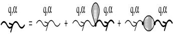
Figure 1: The Dyson equation for the photon Green function. The bare second-order (first-order) electron-photon coupling leads to the second (third) term on the right-hand side, giving rise to the diamagnetic (current-current) contribution to the photon self-energy.

The following general properties of the expression (8) are important for interpreting the measured spectra. First, there are at least two distinct structures in the optical conductivity spectrum ${\rm Re}\{\sigma_{\alpha\alpha}(\omega)\}$, the first one is a delta function at $\omega=0$, related to the diamagnetic current, and the second one represents various contributions, including the exciton contributions if the short-range dipole-dipole interactions are present Wooten (2, 16, 17, 18). This is easily seen from

$${\rm Re}\{\sigma_{\alpha\alpha}(\omega)\} = \frac{1}{4}\big{[}\Omega_{{\rm dia},\alpha}^{2}+4\pi{\rm Re}\{\Pi_{\alpha\alpha}(0)\}\big{]}\delta(\omega)$$ (9)

$$-\frac{1}{\omega}{\rm Im}\{\Pi_{\alpha\alpha}(\omega)\}.$$

Obviously, in the normal metallic or insulating state the delta-function term vanishes Kittel (13). Therefore, any consistent treatment of the electron-photon coupling functions has to fulfill the relation

$$\Omega_{{\rm dia},\alpha}^{2}+4\pi{\rm Re}\{\Pi_{\alpha\alpha}(0)\}=0.$$ (10)

The total optical conductivity in the normal metallic or insulating state can be written then in the form

$$\sigma_{\alpha\alpha}(\omega) = \frac{\rm i}{\omega}\big{[}\Pi_{\alpha\alpha}(\omega)-{\rm Re}\{\Pi_{\alpha\alpha}(0)\}\big{]}.$$ (11)

Noteworthy, in the superconducting state the sum

$$\frac{1}{2}\big{[}\Omega_{{\rm dia},\alpha}^{2}+4\pi{\rm Re}\{\Pi_{\alpha\alpha}(0)\}\big{]}$$ (12)

measures the weight of the missing area in optical conductivity spectra Schrieffer (19, 20, 21), while the single-particle contributions are still given by Eq. (11). Finally, notice that in absence of local dipolar excitations (the case of the site-energy dimerization discussed in this article) the total current-current correlation function is the sum of only two contributions describing, respectively, the creation of the “free” intra- and interband electron-hole pairs, while the processes associated with excitons (i.e. the quasiparticles representing the bound electron-hole pairs) are not present.

The optical conductivity determined by Eq. (11), with the current-current correlation function calculated by the equation of motion approach, is in the focus of the present analysis. The causality requirement Wooten (2, 13) (i.e. the Kramers–Kronig relations), the effective mass theorem KupcicPB1 (4, 22, 23) and the gauge-invariance requirement KupcicPB1 (4, 11, 15) will be used to test the obtained results. A particular care will be devoted to the non-physical singularity at $\omega=0$ related to the prefactor of $\omega^{-1}$ in Eq. (11), and to the construction of the optical conductivity model with the correct behaviour in the $\omega\rightarrow 0$ limit, giving rise to a unified description of the optical and transport phenomena.

III Electronic Hamiltonian with two qualitatively different scattering channels

Although our model is Q1D, the present response theory is quite general and the electronic Hamiltonian could represent an arbitrary multiband model. We assume that in addition to the bare electronic Hamiltonian (denoted below by ${H}_{0}$) there is a static single-particle potential (${H}^{\prime}_{0}$) characterized by a commensurate wave vector, which describes, for example, the scattering of electrons on the site-energy dimerization potential. The other single-electron scattering processes (on impurities, phonons, etc.) are represented by ${H}^{\prime}_{1}$. For most of the questions discussed here the main effects of the two-electron interactions are taken satisfactorily into account through the effective mean fields included in ${H}^{\prime}_{0}$ or ${H}^{\prime}_{1}$, footnote2 (24) resulting finally in $H^{\rm el}_{0}={H}_{0}+{H}^{\prime}_{0}+{H}^{\prime}_{1}$ in Eq. (1). $H^{\rm ext}=H^{\rm ext}_{1}+H^{\rm ext}_{2}$ couples the valence electrons to transverse electromagnetic fields. The resulting total electronic Hamiltonian is

$$H^{\rm el} = H^{\rm el}_{0}+H^{\rm ext}.$$ (13)

We start by diagonalizing the Hamiltonian ${H}_{0}+{H}^{\prime}_{0}$. As mentioned above, we consider the simplest Q1D model, where ${H}^{\prime}_{0}$ represents the site-energy dimerization in the highly conducting direction and in ${H}^{\prime}_{1}$ only the impurity scattering is taken into account. Next, we determine the related electron-photon coupling functions. At the end of this section, the multiband current-current correlation function is introduced.

III.1 Bare Hamiltonian

The single-particle properties of the Q1D site-energy-dimerization model come from the exact diagonalization of the Hamiltonian KupcicPB2 (15)

$${H}_{0}+{H}^{\prime}_{0} = \sum_{{\bf k}\sigma}\big{[}\varepsilon_{c}({\bf k})c^{\dagger}_{{\bf k}\sigma}c_{{\bf k}\sigma}+\varepsilon_{\underline{c}}({\bf k})\underline{c}^{\dagger}_{{\bf k}\sigma}\underline{c}_{{\bf k}\sigma}$$ (14)

$$\hskip 28.45274pt+\Delta\big{(}\underline{c}^{\dagger}_{{\bf k}\sigma}c_{{\bf k}\sigma}+c^{\dagger}_{{\bf k}\sigma}\underline{c}_{{\bf k}\sigma}\big{)}\big{]}.$$

The bare electron dispersions of two subbands, artificially dimerized along the highly conducting direction $a$, are

$$\varepsilon_{\underline{c},c}({\bf k}) = \pm 2t_{a}\cos{\bf k}\cdot{\bf a}-2t_{b}\cos{\bf k}\cdot{\bf b},$$ (15)

with $\varepsilon_{\underline{c}}({\bf k})\equiv\varepsilon_{c}({\bf k}\pm\pi/a\hat{x})$, and with the wave vector k restricted to the new (reduced) Brillouin zone, $-0.5\pi/a\leq k_{x}\leq 0.5\pi/a$, $-\pi/b\leq k_{y}\leq\pi/b$. $t_{a}$ and $t_{b}$ ($t_{a}\gg t_{b}>0$) are the bond energies in the direction $a$ and the perpendicular direction $b$, respectively, and $\Delta$ is the magnitude of the dimerization potential in the direction $a$. Note that such potential corresponds to imperfect nesting in Eq. (15) in contrast to dimerization in all directions; the former nesting is chosen because it is more interesting in context of the conductivity studies.

The transformations between the unperturbed states, the band index $l=c,\underline{c}$, and the Bloch states, the band index $L=C,\underline{C}$, of the form

$$l_{{\bf k}\sigma}^{\dagger} = \sum_{L}U_{\bf k}(l,L)L_{{\bf k}\sigma}^{\dagger},$$ (16)

lead to

$$H_{0} = \sum_{L{\bf k}\sigma}E_{L}({\bf k})L_{{\bf k}\sigma}^{\dagger}L_{{\bf k}\sigma},$$ (17)

with the dispersions

$$E_{\underline{C},C}({\bf k}) = \frac{1}{2}[\varepsilon_{\underline{c}}({\bf k})+\varepsilon_{c}({\bf k})]\pm\sqrt{\frac{1}{4}\varepsilon_{\underline{c}c}^{2}({\bf k})+\Delta^{2}},$$

$$\varepsilon_{\underline{c}c}({\bf k}) = \varepsilon_{\underline{c}}({\bf k})-\varepsilon_{c}({\bf k}).$$ (18)

The transformation-matrix elements are given by

$$\left(\begin{array}[]{ll}U_{\bf k}(c,C)&U_{\bf k}(c,\underline{C})\\ U_{\bf k}(\underline{c},C)&U_{\bf k}(\underline{c},\underline{C})\end{array}\right) = \left(\begin{array}[]{cc}u({\bf k})&v({\bf k})\\ -v({\bf k})&u({\bf k})\end{array}\right),$$ (23)

where $u({\bf k})=\displaystyle\cos\frac{\varphi({\bf k})}{2}$, $v({\bf k})=\displaystyle\sin\frac{\varphi({\bf k})}{2}$, with the auxiliary phase $\varphi({\bf k})$ defined in the usual way

$$\tan\varphi({\bf k}) = \frac{2\Delta}{\varepsilon_{\underline{c}c}({\bf k})}.$$ (24)

The bands are shown in Fig. 2. Hereafter, the lower (conduction) band is assumed to be partially filled and the upper (valence) band is empty. For the lower band completely filled and $\Delta\gg t_{b}$, the band structure corresponds to the commensurate CDW system, otherwise we have the metallic behaviour.

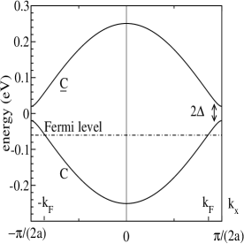
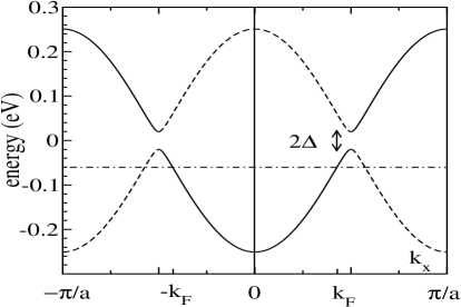
Figure 2: The electron dispersions $E_{\underline{C},C}(k_{x},0.5\pi/b)$ in the reduced (a) and extended (b) zone representation, for $2t_{a}=0.25$ eV and $\Delta=0.02$ eV. In Fig. (b), the solid and dashed lines correspond, respectively, to $u({\bf k})$ and $v({\bf k})$ in the relations $C^{\dagger}_{{\bf k}\sigma}=u({\bf k})c^{\dagger}_{{\bf k}\sigma}-v({\bf k})\underline{c}^{\dagger}_{{\bf k}\sigma}$, $\underline{C}^{\dagger}_{{\bf k}\sigma}=v({\bf k})c^{\dagger}_{{\bf k}\sigma}+u({\bf k})\underline{c}^{\dagger}_{{\bf k}\sigma}$. The dot-dashed line is the Fermi level $\mu$ in a typical metallic case.

III.2 Electron-photon coupling Hamiltonian

Using the generalized minimal substitution method for the tight-binding electrons KupcicPB1 (4, 15), we obtain that the conduction electrons described by the Hamiltonian (14) are coupled to the external electromagnetic fields through

$$H^{\rm ext} = \sum_{l}\sum_{{\bf k}\sigma}\sum_{{\bf q}\alpha}\delta H_{0}^{l}({\bf k},{\bf q})l_{{\bf k}+{\bf q}\sigma}^{\dagger}l_{{\bf k}\sigma},$$ (25)

where, to the second order in the vector potential $A_{\alpha}({\bf q})$,

$$\delta H_{0}^{l}({\bf k},{\bf q}) \approx -\frac{\partial\varepsilon_{l}({\bf k})}{\partial k_{\alpha}}\frac{e}{\hbar c}A_{\alpha}({\bf q})+\frac{1}{2}\frac{\partial^{2}\varepsilon_{l}({\bf k})}{\partial k_{\alpha}^{2}}\bigg{(}\frac{e}{\hbar c}\bigg{)}^{2}A_{\alpha}^{2}({\bf q}).$$

The photon annihilation operator $A_{{\bf q}\alpha}$ enters in Eq. (LABEL:eq22) through

$$A_{\alpha}({\bf q})\hskip 5.69054pt=\hskip 5.69054pt\sqrt{\frac{4\pi c^{2}}{V}}Q_{{\bf q}\alpha},$$

$$A_{\alpha}^{2}({\bf q})\hskip 5.69054pt=\hskip 5.69054pt\sum_{{\bf q}^{\prime}}A_{\alpha}({\bf q}-{\bf q}^{\prime})A_{\alpha}({\bf q}^{\prime}),$$

where

$$Q_{{\bf q}\alpha} = \sqrt{\frac{\hbar}{2\omega_{{\bf q}\alpha}}}\big{[}A_{{\bf q}\alpha}+A^{\dagger}_{-{\bf q}\alpha}\big{]}$$ (27)

is the electromagnetic displacement field of Eq. (2) Pines (11). Finally, in the Bloch representation the coupling Hamiltonian becomes

$$H^{\rm ext} = H^{\rm ext}_{1}+H^{\rm ext}_{2}=-\frac{1}{c}\sum_{{\bf q}\alpha}A_{\alpha}({\bf q})\hat{J}_{\alpha}(-{\bf q})$$ (28)

$$\hskip 14.22636pt+\frac{{e}^{2}}{2mc^{2}}\sum_{{\bf q}\alpha}A^{2}_{\alpha}({\bf q})\hat{\gamma}_{\alpha\alpha}(-{\bf q};2),$$

with

$$\hskip 22.76219pt\hat{J}_{\alpha}({\bf q}) = \sum_{LL^{\prime}}\sum_{{\bf k}\sigma}J^{LL^{\prime}}_{\alpha}({\bf k})L_{{\bf k}\sigma}^{\dagger}L^{\prime}_{{\bf k}+{\bf q}\sigma},$$ (29)

$$\hskip 22.76219pt\hat{\gamma}_{\alpha\alpha}({\bf q};2) = \sum_{LL^{\prime}}\sum_{{\bf k}\sigma}\gamma^{LL^{\prime}}_{\alpha\alpha}({\bf k};2)L_{{\bf k}\sigma}^{\dagger}L^{\prime}_{{\bf k}+{\bf q}\sigma},\hskip 14.22636pt(25^{\prime})$$

representing, respectively, the current density and Raman Genkin (22, 15) density operators. The structure of the related vertex functions $J^{LL^{\prime}}_{\alpha}({\bf k})$ and $\gamma^{LL^{\prime}}_{\alpha\alpha}({\bf k};2)$ is given in Appendix A.

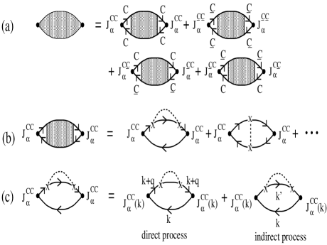
Figure 3: (a) The Bloch representation of the current-current correlation function of the two-band model (14), with the current vertices given by Eqs. (74) and (A2^′). The shaded square is the electron-hole propagator defined by Eq. (32). (b) The intraband current-current correlation function at high-frequencies (the leading term in powers of $(H_{1}^{\prime})^{2}/\omega$). (c) The structure of the high-frequencies self-energy term. The direct processes are associated with the creation of an electron-hole pair with wave vectors k and ${\bf k}+{\bf q}$ (${\bf q}$ is the wave vector of the external field), while the indirect processes involve the impurity-assisted electron-hole pairs with wave vectors ${\bf k}$ and ${\bf k}^{\prime}+{\bf q}\approx{\bf k}^{\prime}$, or ${\bf k}+{\bf q}\approx{\bf k}$ and ${\bf k}^{\prime}$ (${\bf k}^{\prime}-{\bf k}$ is the momentum relaxed on impurities, and the crosses represent the impurity scattering).

III.3 Single-particle scattering processes

We consider here only the intraband impurity scattering processes in the perturbation

$$H_{1}^{\prime} = \sum_{L}\sum_{{\bf k}{\bf k}^{\prime}\sigma}V^{LL}({\bf k},{\bf k}^{\prime})L_{{\bf k}\sigma}^{\dagger}L_{{\bf k}^{\prime}\sigma},$$ (30)

for which one usually assumes $V^{LL}({\bf k},{\bf k}^{\prime})=V^{LL}({\bf k}-{\bf k}^{\prime})$ Abrikosov (8, 9). This form of $H_{1}^{\prime}$ is consistent with the regime in which $\varepsilon_{\underline{c}c}({\bf k}_{\rm F})\gg\hbar/\tau$ ($\tau$ is the relaxation time defined below). The generalization is straightforward.

III.4 Current-current correlation function

In the equation of motion approach Pines (11) used in the next section, the starting point is the current-current correlation function of Eqs. (8)–(12) shown in Fig. 3. It is defined by LRA (1, 2, 7, 15)

$$\Pi_{\alpha\alpha}({\bf q},t) = \frac{1}{\hbar V}\langle\langle\hat{J}_{\alpha}({\bf q});\hat{J}_{\alpha}(-{\bf q})\rangle\rangle_{t}$$ (31)

$$\equiv -\frac{{\rm i}}{\hbar V}\;\Theta(t)\langle\big{[}\hat{J}_{\alpha}({\bf q},t),\hat{J}_{\alpha}(-{\bf q},0)\big{]}\rangle.$$

Here the current operator $\hat{J}_{\alpha}({\bf q})$ includes all intra- and interband current density fluctuations, as seen from Eq. (29). According to Fig. 3, $\Pi_{\alpha\alpha}({\bf q},t)$ comprises two intraband and two interband contributions, and the problem is reduced, as will be seen immediately below, to the self-consistent calculation of intra- and interband electron-hole propagator in presence of the perturbation $H_{1}^{\prime}$. In Eq. (31), as well as in Eqs. (32), (34), (37) and (38), the usual notation for the retarded correlation functions is used: $\langle\langle\hat{A},\hat{B}\rangle\rangle_{t}=-{\rm i}\Theta(t)\langle\big{[}\hat{A}(t),\hat{B}(0)\big{]}\rangle$, with $\hat{A}(t)$ being the operator $\hat{A}$ in the Heisenberg picture.

IV Equation of motion approach

IV.1 Generalized correlation functions

The retarded electron-hole propagator

$$\!\!\!\!\!\!\!\!{\cal D}_{1}^{LL^{\prime}}({\bf k},{\bf k}_{+},{\bf k}_{+}^{\prime},{\bf k}^{\prime},t)=\langle\langle L_{{\bf k}\sigma}^{\dagger}L^{\prime}_{{\bf k}+{\bf q}\sigma};{L^{\prime}}_{{\bf k}^{\prime}+{\bf q}\sigma}^{\dagger}L_{{\bf k}^{\prime}\sigma}\rangle\rangle_{t}$$

$$\hskip 14.22636pt\equiv-{\rm i}\Theta(t)\langle\big{[}\big{(}L_{{\bf k}\sigma}^{\dagger}L^{\prime}_{{\bf k}+{\bf q}\sigma}\big{)}_{t},\big{(}{L^{\prime}}_{{\bf k}^{\prime}+{\bf q}\sigma}^{\dagger}L_{{\bf k}^{\prime}\sigma}\big{)}_{0}]\rangle$$

$$\hskip 14.22636pt={\rm e}^{-\eta t}\frac{1}{2\pi}\int_{-\infty}^{\infty}{\rm d}\omega\,{\rm e}^{{\rm i}\omega t}{\cal D}_{1}^{LL^{\prime}}({\bf k},{\bf k}_{+}^{\prime},{\bf k}_{+},{\bf k}^{\prime},\omega)$$ (32)

(${\bf k}_{+}$ is the abbreviation for ${\bf k}+{\bf q}$) is the central quantity to all long-wavelength correlation functions, as can be seen from Fig. 4, or from the expression

$$\!\!\!\!\!\!\!\!\chi_{f,g}({\bf q},t)=\frac{1}{\hbar V}\sum_{LL^{\prime}}\sum_{{\bf k}{\bf k}^{\prime}\sigma}f^{LL^{\prime}}({\bf k},{\bf k}+{\bf q})g^{L^{\prime}L}({\bf k}^{\prime}+{\bf q},{\bf k}^{\prime})$$

$$\hskip 56.9055pt\times{\cal D}_{1}^{LL^{\prime}}({\bf k},{\bf k}_{+},{\bf k}_{+}^{\prime},{\bf k}^{\prime},t),$$ (33)

which represents a generalized long-wavelength correlation function, with $f^{LL^{\prime}}({\bf k},{\bf k}+{\bf q})$ and $g^{L^{\prime}L}({\bf k}^{\prime}+{\bf q},{\bf k}^{\prime})$ being the charge, current, Raman or some other vertex functions. In Eq. (32) the abbreviation $(\hat{A}\hat{B})_{t}=\hat{A}(t)\hat{B}(t)$ is used.

Figure 4: The generalized correlation function in notations of Fig. 3.

The symmetry of the $f^{LL^{\prime}}({\bf k},{\bf k}+{\bf q})$ and $g^{L^{\prime}L}({\bf k}^{\prime}+{\bf q},{\bf k}^{\prime})$ vertices, together with the nature of the singularity of the leading term in the perturbation series, determines the summation rule for the related Feynman diagrams. The simplest way to collect the most singular diagrams is to consider the equations of motion connecting ${\cal D}_{1}^{LL^{\prime}}({\bf k},{\bf k}_{+},{\bf k}_{+}^{\prime},{\bf k}^{\prime},t)$ with the correlation function ${\cal D}_{2}^{LL^{\prime}}({\bf k},{\bf k}_{+},{\bf k}_{+}^{\prime},{\bf k}^{\prime},t)$ defined as

$$\!\!\!\!\!\!\!\!{\cal D}_{2}^{LL^{\prime}}({\bf k},{\bf k}_{+},{\bf k}_{+}^{\prime},{\bf k}^{\prime},t)$$ (34)

$$\hskip 42.67912pt=\langle\langle\big{[}L_{{\bf k}\sigma}^{\dagger}L^{\prime}_{{\bf k}+{\bf q}\sigma},H^{\prime}];{L^{\prime}}_{{\bf k}^{\prime}+{\bf q}\sigma}^{\dagger}L_{{\bf k}^{\prime}\sigma}\rangle\rangle_{t}.$$

The direct calculation gives the exact relation

$$\hbar\big{[}{\cal D}^{LL^{\prime}}_{0}({\bf k},{\bf k}_{+},\omega)\big{]}^{-1}{\cal D}_{1}^{LL^{\prime}}({\bf k},{\bf k}_{+},{\bf k}_{+}^{\prime},{\bf k}^{\prime},\omega)$$ (35)

$$\hskip 14.22636pt=\hbar\delta_{{\bf k},{\bf k}^{\prime}}\big{[}f_{L}({\bf k})-f_{L^{\prime}}({\bf k}_{+})\big{]}+{\cal D}_{2}^{LL^{\prime}}({\bf k},{\bf k}_{+},{\bf k}_{+}^{\prime},{\bf k}^{\prime},\omega).$$

Here

$$\hbar\big{[}{\cal D}^{LL^{\prime}}_{0}({\bf k},{\bf k}_{+},\omega)\big{]}^{-1}=\hbar(\omega+{\rm i}\eta)+E_{L}({\bf k})-E_{L^{\prime}}({\bf k}_{+})$$

(36)

is a useful abbreviation. ${\cal D}_{2}^{LL^{\prime}}({\bf k},{\bf k}_{+},{\bf k}_{+}^{\prime},{\bf k}^{\prime},\omega)$ is the Fourier transform of ${\cal D}_{2}^{LL^{\prime}}({\bf k},{\bf k}_{+},{\bf k}_{+}^{\prime},{\bf k}^{\prime},t)$, and $f_{L}({\bf k})\equiv f(E_{L}({\bf k}))=\langle{L}_{{\bf k}\sigma}^{\dagger}L_{{\bf k}\sigma}\rangle=\big{[}1+\exp\{\beta[E_{L}({\bf k})-\mu]\}\big{]}^{-1}$ is the Fermi–Dirac function, with $\beta=1/(k_{\rm B}T)$.

The way to evaluate ${\cal D}_{2}^{LL^{\prime}}({\bf k},{\bf k}_{+},{\bf k}_{+}^{\prime},{\bf k}^{\prime},t)$ depends on the choice of representation of this function. There are two alternative ways,

$${\cal D}_{2}^{LL^{\prime}}({\bf k},{\bf k}_{+},{\bf k}_{+}^{\prime},{\bf k}^{\prime},t)$$ (37)

$$\hskip 28.45274pt=-{\rm i}\Theta(t)\langle\big{[}\big{[}L_{{\bf k}\sigma}^{\dagger}L^{\prime}_{{\bf k}+{\bf q}\sigma},H^{\prime}\big{]}_{t},\big{(}{L^{\prime}}_{{\bf k}^{\prime}+{\bf q}\sigma}^{\dagger}L_{{\bf k}^{\prime}\sigma}\big{)}_{0}]\rangle$$

or

$${\cal D}_{2}^{LL^{\prime}}({\bf k},{\bf k}_{+},{\bf k}_{+}^{\prime},{\bf k}^{\prime},t)$$ (38)

$$\hskip 14.22636pt=-{\rm i}\Theta(t)\langle\big{[}\big{[}L_{{\bf k}\sigma}^{\dagger}L^{\prime}_{{\bf k}+{\bf q}\sigma},H^{\prime}\big{]}_{0},\big{(}{L^{\prime}}_{{\bf k}^{\prime}+{\bf q}\sigma}^{\dagger}L_{{\bf k}^{\prime}\sigma}\big{)}_{-t}]\rangle,$$

leading to two different self-consistent schemes (one described below and another encountered in the longitudinal response theory Pines (11)), both giving, as will be argued below, the same result. Again, $[\hat{A},\hat{B}]_{t}$ is the abbreviation for $[\hat{A}(t),\hat{B}(t)]$.

It is important to realize at the outset that the first term on the right-hand side of Eq. (35) is significant for all interband correlation functions $\chi_{f,g}({\bf q},t)$ in Eq. (33), irrespective of the vertex symmetries. The probability for the direct creation of the interband electron-hole pair is proportional here to $f_{L}({\bf k})-f_{L^{\prime}}({\bf k}_{+})\approx f_{L}({\bf k})-f_{L^{\prime}}({\bf k})$, so that all occupied states in the conduction band(s) are equally important. For vertices $f^{LL^{\prime}}({\bf k},{\bf k}+{\bf q})$ and $g^{L^{\prime}L}({\bf k}^{\prime}+{\bf q},{\bf k}^{\prime})$ taken to represent the intraband current vertices, the correlation function $\chi_{f,g}({\bf q},t)$ in Eq. (33) becomes the intraband current-current correlation function $\Pi^{\rm intra}_{\alpha\alpha}({\bf q},t)$. According to the discussion of Sec. II A, the related intraband optical conductivity is ruled by the prefactor $\omega^{-1}$ in Eq. (11). The direct processes in Eq. (35) (see the first term on the right-hand side of Fig. 3(c)) related to $f_{C}({\bf k})-f_{C}({\bf k}_{+})\rightarrow 0$ are insignificant, and $\Pi^{\rm intra}_{\alpha\alpha}({\bf q},t)$ can be adequately described by the second, indirect term in this equation (the second term in Fig. 3(c); see also Fig. 5), with ${\cal D}_{2}^{LL^{\prime}}({\bf k},{\bf k}_{+},{\bf k}_{+}^{\prime},{\bf k}^{\prime},t)$ given by Eq. (38).

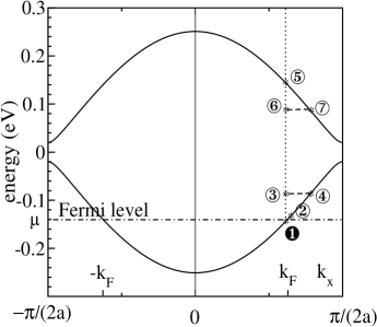
Figure 5: The direct intraband ($1\rightarrow 2$), indirect intraband ($1\rightarrow 3\rightarrow 4$), direct interband ($1\rightarrow 5$) and indirect interband ($1\rightarrow 6\rightarrow 7$) optical excitations. In this article the second and third processes are considered, the indirect intraband, using the exact summation of the impurity scattering processes, and the direct interband, using the phenomenological treatment of the impurity scattering. The dotted line is the photon dispersion, and the dashed line corresponds to the impurity scattering.

Before turning to the evaluation of $\Pi^{\rm intra}_{\alpha\alpha}({\bf q},t)$ it is interesting to contrast this conclusion with its analog in the longitudinal response theory. In the longitudinal approach, the long-range Coulomb forces are activated, and the first term in Eq. (35) dominates the intraband charge-charge correlation function, even in the dynamic limit, since the small probability for the intraband electron-hole pair creation, proportional to $f_{C}({\bf k})-f_{C}({\bf k}_{+})$, cancels out the $q^{-2}$ singularity of the long-range forces, which is the well-known RPA result. The indirect scattering processes, on the other hand, are proportional to the effective intraband charge vertex, analogous to the effective intraband current vertex introduced below, Eq. (45). Since the bare long-wavelength intraband charge vertex satisfies $q({\bf k}+{\bf q},{\bf k})\approx q({\bf k},{\bf k})=e$, where $e$ is the bare electron charge, the effective intraband charge vertex for the indirect scattering processes vanishes, because $q({\bf k},{\bf k})-q({\bf k}^{\prime},{\bf k}^{\prime})=0$. Since the longitudinal and transverse approaches are to be equivalent, this means that the direct longitudinal processes are to be equivalent to the indirect transverse processes in the intraband channel, while the contributions of both the indirect longitudinal and the direct transverse scattering processes are to be negligible. This issue will be further discussed in Sec. IV B 5.

The above transverse approach can now be applied to the current-current correlation function of the two band model, rewritten in the form

$$\Pi_{\alpha\alpha}({\bf q},t) = \frac{1}{\hbar V}\sum_{LL^{\prime}}\sum_{{\bf k}{\bf k}^{\prime}\sigma}J^{LL^{\prime}}_{\alpha}({\bf k})J^{L^{\prime}L}_{\alpha}({\bf k}^{\prime})$$ (39)

$$\hskip 14.22636pt\times{\cal D}_{1}^{LL^{\prime}}({\bf k},{\bf k}_{+},{\bf k}_{+}^{\prime},{\bf k}^{\prime},t).$$

Here the vertices $f^{LL^{\prime}}({\bf k},{\bf k}+{\bf q})$ and $g^{L^{\prime}L}({\bf k}^{\prime}+{\bf q},{\bf k}^{\prime})$ in Eq. (33) are replaced by $J^{LL^{\prime}}_{\alpha}({\bf k},{\bf k}+{\bf q})\approx J^{LL^{\prime}}_{\alpha}({\bf k})$ and $J^{L^{\prime}L}_{\alpha}({\bf k}^{\prime}+{\bf q},{\bf k}^{\prime})\approx J^{L^{\prime}L}_{\alpha}({\bf k}^{\prime})$, respectively. Optical processes relevant to the two-band model (including the indirect interband ones not considered in the present analysis) are illustrated in Fig. 5.

In order to make presentation of the results more transparent, we shall first determine the intraband contributions, and then give the analysis of the interband optical excitations. For the sake of brevity, in the next section the (intra)band index $C$ will be omitted ($E_{C}({\bf k})\rightarrow E({\bf k})$, $J^{CC}_{\alpha}({\bf k})\rightarrow J_{\alpha}({\bf k})$, …, with $C_{{\bf k}\sigma}^{\dagger}\rightarrow c_{{\bf k}\sigma}^{\dagger}$). It should be noticed that the results obtained below for the intraband optical conductivity are quite general, i.e. they cover various physically different regimes. As explained in Sec. IV B 2, when the electron filling of the dimerized band varies between 0 and 1, the electronic system transforms from an electron-like semiconducting, through a metallic, into a hole-like semiconducting regime. A more detailed discussion of this issue is given in Sec. V, in context of the total optical conductivity.

IV.2 Intraband optical conductivity

According to the aforementioned arguments, the intraband optical processes are described by the equations

$$\!\!\!\!\!\!\!\!\hbar{\cal D}_{0}^{-1}({\bf k},{\bf k}_{+},\omega){\cal D}_{1}({\bf k},{\bf k}_{+},{\bf k}_{+}^{\prime},{\bf k}^{\prime},\omega)$$

$$\hskip 71.13188pt={\cal D}_{2}({\bf k},{\bf k}_{+},{\bf k}_{+}^{\prime},{\bf k}^{\prime},\omega),$$ (40)

$$\!\!\!\!\!\!\!\!\hbar{\cal D}_{0}^{-1}({\bf k}^{\prime},{\bf k}^{\prime}_{+},\omega){\cal D}_{2}({\bf k},{\bf k}_{+},{\bf k}_{+}^{\prime},{\bf k}^{\prime},\omega)$$

$$\hskip 28.45274pt=-{\cal D}_{3}({\bf k},{\bf k}_{+},{\bf k}_{+}^{\prime},{\bf k}^{\prime},\omega)$$

$$\hskip 42.67912pt+\hbar\langle\big{[}\big{[}c_{{\bf k}\sigma}^{\dagger}c_{{\bf k}+{\bf q}\sigma},H^{\prime}\big{]},{c}_{{\bf k}^{\prime}+{\bf q}\sigma}^{\dagger}c_{{\bf k}^{\prime}\sigma}]\rangle,$$ (41)

where ${\cal D}_{0}^{-1}({\bf k}^{\prime},{\bf k}^{\prime}_{+},\omega)$ is the intraband term in Eq. (36) and ${\cal D}_{3}({\bf k},{\bf k}_{+},{\bf k}_{+}^{\prime},{\bf k}^{\prime},\omega)$ is the Fourier transform of the force-force correlation function Mahan (7, 25, 15)

$${\cal D}_{3}({\bf k},{\bf k}_{+},{\bf k}_{+}^{\prime},{\bf k}^{\prime},t)$$ (42)

$$\hskip 14.22636pt=-{\rm i}\Theta(t)\langle\big{[}\big{[}c_{{\bf k}\sigma}^{\dagger}c_{{\bf k}+{\bf q}\sigma},H^{\prime}\big{]}_{0},\big{[}c_{{\bf k}^{\prime}+{\bf q}\sigma}^{\dagger}c_{{\bf k}^{\prime}\sigma},\,H^{\prime}\big{]}_{-t}]\rangle.$$

The second term in Eq. (41) is the ground-state average of the four-operator product at $t=0$. It is off-diagonal in the Bloch representation, and its value can be obtained by putting $E({\bf k}^{\prime}_{+})-E({\bf k}^{\prime})\approx 0$ in the left-hand side of Eq. (41) and then taking the formal limit $\omega\rightarrow 0$. The result is

$$\!\!\!\!\!\!\!\!\hbar\langle\big{[}\big{[}c_{{\bf k}\sigma}^{\dagger}c_{{\bf k}+{\bf q}\sigma},H^{\prime}\big{]},{c}_{{\bf k}^{\prime}+{\bf q}\sigma}^{\dagger}c_{{\bf k}^{\prime}\sigma}]\rangle$$

$$\hskip 56.9055pt\approx{\cal D}_{3}({\bf k},{\bf k}_{+},{\bf k}_{+}^{\prime},{\bf k}^{\prime},\omega=0).$$ (43)

For the impurity scattering, we have the cancellation of this constant term with its counterpart obtained by the electron $\rightleftharpoons$ hole replacement (see Eq. (51), for example), but for a time-dependent perturbation $H_{1}^{\prime}$, Eq. (43) achieves an interesting structure, as pointed out in Refs. Gotze (25, 26)

Due to the large velocity of light, the energy and wave vector transfers in the external points of the intraband current-current correlation function fulfill $\hbar\omega\gg E({\bf k}^{\prime}_{+})-E({\bf k}^{\prime})$, and the factors ${\cal D}_{0}({\bf k},{\bf k}_{+},\omega)$ and ${\cal D}_{0}({\bf k}^{\prime},{\bf k}^{\prime}_{+},\omega)$ in Eqs. (40) and (41), representing the propagator of the virtual electron-hole pairs (related to the process $1\rightarrow 3$ in Fig. 5), can be replaced by $1/\omega$. The resulting intraband correlation function becomes

$$\Pi^{\rm intra}_{\alpha\alpha}(\omega)=-\frac{1}{\hbar V(\hbar\omega)^{2}}\sum_{{\bf k}{\bf k}^{\prime\prime}{\bf k}_{1}{\bf k}^{\prime\prime}_{1}\sigma}\big{[}J_{\alpha}({\bf k})-J_{\alpha}({\bf k}^{\prime\prime})\big{]}$$

$$\hskip 28.45274pt\times\big{[}J_{\alpha}({\bf k}^{\prime\prime}_{1})-J_{\alpha}({\bf k}_{1})\big{]}\bigg{<}V({\bf k}-{\bf k}^{\prime\prime})V({\bf k}^{\prime\prime}_{1}-{\bf k}_{1})$$

$$\times\big{[}{\cal D}_{1}({\bf k},{\bf k}^{\prime\prime},{\bf k}_{1}^{\prime\prime},{\bf k}_{1},\omega)-{\cal D}_{1}({\bf k},{\bf k}^{\prime\prime},{\bf k}_{1}^{\prime\prime},{\bf k}_{1},0)\big{]}\bigg{>}.$$ (44)

$\langle\ldots\rangle$ is here and subsequently the average over the impurity sites Mahan (7).

Figure 6: (a) The indirect contributions to the intraband current-current correlation function in the equation of motion approach. The open square is the effective current vertex, and the dashed line represents the related force-force correlation functions (see, for example, the discussion of the force-force correlation function method in Sec. 8.1.B of Ref. Mahan (7)). (b) The leading term in the high-frequency limit. On the right-hand side, the products $V({\bf k}-{\bf k}^{\prime\prime})J_{\alpha}({\bf k})/(\hbar\omega)$ and $V({\bf k}-{\bf k}^{\prime\prime})J_{\alpha}({\bf k}^{\prime\prime})/(\hbar\omega)$ are encircled into the effective vertex. The dot is the bare intraband current vertex.

The diagrammatic representation of $\Pi^{\rm intra}_{\alpha\alpha}({\bf q},\omega)$ is given in Fig. 6(a), with the structure of the leading term, proportional to $(H_{1}^{\prime})^{2}/\omega$, shown explicitly in Fig. 6(b). The expression

$$j_{\alpha}({\bf k},{\bf k}^{\prime\prime}) = \frac{V({\bf k}-{\bf k}^{\prime\prime})}{\hbar\omega}\big{[}J_{\alpha}({\bf k})-J_{\alpha}({\bf k}^{\prime\prime})\big{]}$$ (45)

can be recognized as an effective current vertex for the indirect intraband photon absorption/emission processes, and is a sum of two terms encircled in Fig. 6(b). Notice also that ${\cal D}_{1}({\bf k},{\bf k}^{\prime\prime},{\bf k}_{1}^{\prime\prime},{\bf k}_{1},\omega)-{\cal D}_{1}({\bf k},{\bf k}^{\prime\prime},{\bf k}_{1}^{\prime\prime},{\bf k}_{1},0)$ is proportional to $\omega$, canceling out the factor of $\omega^{-1}$ in one of the effective vertices.

It is important to notice that in the leading term (Fig. 6(b)) the expression (44) is identical to the result of the force-force correlation function method Mahan (7). While the latter method is usually limited to the examination of this leading term, or to the summation of irrelevant higher order diagrams which results in the well-known Hopfield formula Mahan (7), the present approach is focused instead on the exact summation of the most singular contributions in powers of $(H_{1}^{\prime})^{2}/\omega$ and should be regarded as a generalization of the standard force-force correlation function approach.

IV.2.1 Proper electron-hole representation

After determining the structure of the external points (i.e. the effective vertices) in the diagram shown in Fig. 6(a), we have to find the internal structure of the diagram. The latter is represented by the indirect (impurity-assisted) electron-hole propagator ${\cal D}_{1}({\bf k},{\bf k}^{\prime\prime},{\bf k}_{1}^{\prime\prime},{\bf k}_{1},\omega)$, characterized by the momentum transfer ${\bf k}-{\bf k}^{\prime\prime}$, rather than by the negligibly small external momentum transfer ${\bf k}_{+}-{\bf k}={\bf q}$ of the direct processes in Eq. (35). Its internal structure is determined here by the self-consistent solution of the exact equation

$$\!\!\!\!\!\!\!\!\hbar{\cal D}^{-1}_{0}({\bf k},{\bf k}^{\prime\prime},\omega){\cal D}_{1}({\bf k},{\bf k}^{\prime\prime},{\bf k}_{1}^{\prime\prime},{\bf k}_{1},\omega)$$ (46)

$$=\hbar\delta_{{\bf k},{\bf k}_{1}}\delta_{{\bf k}^{\prime\prime},{\bf k}_{1}^{\prime\prime}}\big{[}f({\bf k})-f({\bf k}^{\prime\prime})\big{]}+{\cal D}_{2}({\bf k},{\bf k}^{\prime\prime},{\bf k}_{1}^{\prime\prime},{\bf k}_{1},\omega).$$

${\cal D}_{1}({\bf k},{\bf k}^{\prime\prime},{\bf k}_{1}^{\prime\prime},{\bf k}_{1},\omega)$ represents the electron-hole pair created by the indirect photon absorption of Fig. 5, which means that the energy transfer $\hbar\omega$ is close to the electron-hole pair energy $E({\bf k})-E({\bf k}^{\prime\prime})$. The wave vectors k and ${\bf k}^{\prime\prime}$ (${\bf k}_{1}$ and ${\bf k}^{\prime\prime}_{1}$, as well) are independent of each other, and therefore the first term in Eq. (46) dominates the low-energy physics, preferring the optical processes between the states $E({\bf k})\approx\mu$ and $E({\bf k}^{\prime\prime})\approx\mu$.

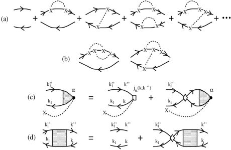
Figure 7: (a) A few leading contributions included in the self-consistent treatment of Eq. (46). (b) Typical contributions omitted in the self-consistent scheme. (c) The self-consistent equation of the kernel ${\cal F}_{\alpha}({\bf k}^{\prime\prime}_{1},{\bf k}_{1},\omega)$ and (d) of the electron-hole propagator ${\cal D}_{1}({\bf k},{\bf k}^{\prime\prime},{\bf k}_{1}^{\prime\prime},{\bf k}_{1},\omega)$. The diamond represents the electron-hole self-energy consisting of the single-particle self-energy and vertex-correction contributions.

In combining Eq. (46) with the equation of motion for ${\cal D}_{2}({\bf k},{\bf k}^{\prime\prime},{\bf k}_{1}^{\prime\prime},{\bf k}_{1},\omega)$ (see Eq. (57) for more detail) it is sufficient to collect only the terms in the summation which are relevant to the self-consistent equation for the kernel ${\cal F}_{\alpha}({\bf k}_{1}^{\prime\prime},{\bf k}_{1},\omega)$ in the current-current correlation function (see Figs. 7(c,d), and the criterion of the validity shown in Figs. 7(a,b))

$$\Pi^{\rm intra}_{\alpha\alpha}(\omega)=-\frac{1}{\hbar V(\hbar\omega)^{2}}\sum_{{\bf k}_{1}{\bf k}^{\prime\prime}_{1}\sigma}\bigg{<}\big{[}J_{\alpha}({\bf k}^{\prime\prime}_{1})-J_{\alpha}({\bf k}_{1})\big{]}$$

$$\hskip 42.67912pt\times\big{[}{\cal F}_{\alpha}({\bf k}_{1}^{\prime\prime},{\bf k}_{1},\omega)-{\cal F}_{\alpha}({\bf k}_{1}^{\prime\prime},{\bf k}_{1},0)\big{]}\bigg{>},$$ (47)

where

$$\!\!\!\!\!\!\!\!{\cal F}_{\alpha}({\bf k}_{1}^{\prime\prime},{\bf k}_{1},\omega)=\sum_{{\bf k}{\bf k}^{\prime\prime}}V({\bf k}-{\bf k}^{\prime\prime})V({\bf k}^{\prime\prime}_{1}-{\bf k}_{1})$$

$$\hskip 14.22636pt\times\big{[}J_{\alpha}({\bf k})-J_{\alpha}({\bf k}^{\prime\prime})\big{]}{\cal D}_{1}({\bf k},{\bf k}^{\prime\prime},{\bf k}_{1}^{\prime\prime},{\bf k}_{1},\omega).$$ (48)

The idea of the present approach is the self-consistent treatment of Eqs. (46) and (IV.2.1), which represent two equations connecting the electron-hole propagator ${\cal D}_{1}({\bf k},{\bf k}^{\prime\prime},{\bf k}_{1}^{\prime\prime},{\bf k}_{1},\omega)$ with the kernel ${\cal F}_{\alpha}({\bf k}_{1}^{\prime\prime},{\bf k}_{1},\omega)$. The solution is based on the expansion

$${\cal D}_{1}({\bf k},{\bf k}^{\prime\prime},{\bf k}_{1}^{\prime\prime},{\bf k}_{1},\omega)=\sum_{n=0}^{\infty}{\cal D}_{1}^{(2n)}({\bf k},{\bf k}^{\prime\prime},{\bf k}_{1}^{\prime\prime},{\bf k}_{1},\omega),$$ (49)

where ${\cal D}_{1}^{(2n)}({\bf k},{\bf k}^{\prime\prime},{\bf k}_{1}^{\prime\prime},{\bf k}_{1},\omega)$ includes only the self-consistent terms proportional to $(H_{1}^{\prime})^{2n}/\omega^{n}$.

As easily seen in the longitudinal analysis, the self-consistent expression for ${\cal D}_{1}({\bf k},{\bf k}^{\prime\prime},{\bf k}_{1}^{\prime\prime},{\bf k}_{1},\omega)$, with ${\bf k}^{\prime\prime}\rightarrow{\bf k}+{\bf q}$, plays the leading role. Accordingly, to compare both response theories, one needs the self-consistent scheme for ${\cal F}_{\alpha}({\bf k}_{1}^{\prime\prime},{\bf k}_{1},\omega)$ and the recurrence relations for ${\cal D}_{1}^{(2n)}({\bf k},{\bf k}^{\prime\prime},{\bf k}_{1}^{\prime\prime},{\bf k}_{1},\omega)$ (see Sec. IV B 3).

For pedagogical reasons, it is convenient first to consider the zeroth order contribution to (47) and define the effective number of conduction electrons and the related electron-hole damping energy.

IV.2.2 High-frequency limit

The direct calculation gives the first term in the expansion (49)

$${\cal D}_{1}^{(0)}({\bf k},{\bf k}^{\prime\prime},{\bf k}_{1}^{\prime\prime},{\bf k}_{1},\omega)$$ (50)

$$\hskip 28.45274pt=\delta_{{\bf k},{\bf k}_{1}}\delta_{{\bf k}^{\prime\prime},{\bf k}_{1}^{\prime\prime}}\big{[}f({\bf k})-f({\bf k}^{\prime\prime})\big{]}{\cal D}_{0}({\bf k},{\bf k}^{\prime\prime},\omega).$$

The related contribution to the current-current correlation function (which is a good approximation for $\Pi^{\rm intra}_{\alpha\alpha}(\omega)$ at high frequencies) is given by

$$\Pi^{\rm intra,(0)}_{\alpha\alpha}(\omega)=\frac{1}{\big{(}\hbar\omega\big{)}^{2}}\frac{1}{V}\sum_{{\bf k}{\bf k}^{\prime\prime}\sigma}J_{\alpha}({\bf k})\big{(}J_{\alpha}({\bf k})-J_{\alpha}({\bf k}^{\prime\prime})\big{)}$$

$$\hskip 28.45274pt\times\big{[}f({\bf k})-f({\bf k}^{\prime\prime})\big{]}\langle|V({\bf k}-{\bf k}^{\prime\prime})|^{2}\rangle$$

$$\hskip 56.9055pt\times\frac{1}{\hbar}\big{[}{\cal D}_{0}({\bf k},{\bf k}^{\prime\prime},\omega)-{\cal D}_{0}({\bf k}^{\prime\prime},{\bf k},\omega)\big{]}$$ (51)

$$\hskip 28.45274pt\approx\frac{1}{\big{(}\hbar\omega\big{)}^{2}}\frac{1}{V}\sum_{{\bf k}{\bf k}^{\prime\prime}\sigma}J_{\alpha}({\bf k})\big{(}J_{\alpha}({\bf k})-J_{\alpha}({\bf k}^{\prime\prime})\big{)}$$

$$\hskip 42.67912pt\times\big{[}f(E({\bf k}))-f(E({\bf k})+\hbar\omega)\big{]}\langle|V({\bf k}-{\bf k}^{\prime\prime})|^{2}\rangle$$

$$\hskip 56.9055pt\times\frac{1}{\hbar}\big{[}{\cal D}_{0}({\bf k},{\bf k}^{\prime\prime},\omega)+{\cal D}_{0}({\bf k}^{\prime\prime},{\bf k},\omega)\big{]}.\hskip 14.22636pt(47^{\prime})$$

For the impurity scattering processes, the real part of this function is negligible, while the imaginary part is given by

$${\rm Im}\{\Pi^{\rm intra(0)}_{\alpha\alpha}(\omega)\}\approx-\frac{1}{\big{(}\hbar\omega\big{)}^{2}}\frac{1}{V}\sum_{{\bf k}\sigma}J^{2}_{\alpha}({\bf k})$$ (52)

$$\hskip 56.9055pt\times\big{[}f(E({\bf k}))-f(E({\bf k})+\hbar\omega)\big{]}\frac{\hbar}{\tau({\bf k},\omega)},$$

where the electron-hole damping energy is

$$\frac{\hbar}{\tau({\bf k},\omega)}=\sum_{{\bf k}^{\prime\prime}}\langle|V({\bf k}-{\bf k}^{\prime\prime})|^{2}\rangle\bigg{(}1-\frac{J_{\alpha}({\bf k}^{\prime\prime})}{J_{\alpha}({\bf k})}\bigg{)}$$

$$\hskip 56.9055pt\times(-)\frac{2}{\hbar}{\rm Im}\big{\{}{\cal D}_{0}({\bf k},{\bf k}^{\prime\prime},\omega)\big{\}}.$$ (53)

Furthermore, in this case, the frequency dependent part in $1/\tau({\bf k},\omega)$ is negligibly small, and we can put the average over the Fermi surface $\langle 1/\tau({\bf k},0)\rangle_{\rm FS}\equiv 1/\tau$ in Eq. (52) instead of $1/\tau({\bf k},\omega)$. We finally get KupcicPB2 (15)

$${\rm Im}\{\Pi^{\rm intra,(0)}_{\alpha\alpha}(\omega)\}\approx-\frac{e^{2}n^{\rm eff}_{\rm intra,\alpha}}{m}\frac{1}{\omega\tau},$$ (54)

with

$$n^{\rm eff}_{\rm intra,\alpha} = -\frac{m}{e^{2}}\frac{1}{V}\sum_{{\bf k}\sigma}J^{2}_{\alpha}({\bf k})\frac{\partial f({\bf k})}{\partial E({\bf k})}$$ (55)

being the effective number of conduction electrons. The behaviour of $n^{\rm eff}_{\rm intra,a}$ with band filling $\delta$ is shown in Fig. 8 for a few typical values of the ratio $\Delta/(2t_{a})$, and compared to the prediction of the free-electron and free-hole approximation. Notice that for $\Delta>2t_{a}\gg 2t_{b}$ one obtains the well-known result $n^{\rm eff}_{\rm intra,a}\propto\sin k_{{\rm F}x}2a=\sin\delta\pi$ ($2a$ is the primitive-cell parameter of the dimerized lattice).

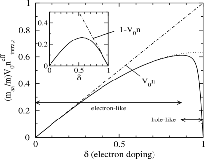
Figure 8: The effective number of conduction electrons (55) shown in the dimensionless form, for $2t_{a}=0.25$ eV, $t_{b}\rightarrow 0$, $T=10$ K and $\Delta=0$ (dotted line), 10 meV (solid line). The dot-dashed line is the dimensionless concentration of conduction electrons $V_{0}n=2ak_{\rm F}/\pi\equiv\delta$, i.e. the prediction of the free-electron approximation. $V_{0}$ is the primitive cell volume and $m_{aa}=\hbar^{2}/(2t_{a}a^{2})$ is the mass scale parameter. The doping regions with the electron-like ($\partial n_{{\rm intra},a}^{\rm eff}/\partial\delta>0$) and hole-like ($\partial n_{{\rm intra},a}^{\rm eff}/\partial\delta<0$) conductivity are also indicated. Inset: The effective number $(m_{aa}/m)V_{0}n_{{\rm intra},a}^{\rm eff}$ for $2t_{a}=0.25$ eV, $t_{b}\rightarrow 0$, $T=10$ K and $\Delta=0.25$ eV. The dot-dashed line is the prediction of the free-hole approximation, $1-V_{0}n$.

Beyond this approximation the expression (51) requires the evaluation of two coupled integrations over k and ${\bf k}^{\prime\prime}$. In the low-dimensional electronic systems, where the van Hove singularities in the band structure may play important role, this is not a trivial task.

The most outstanding advantage of the present approach is the fact that the effective current vertex $j_{\alpha}({\bf k},{\bf k}^{\prime\prime})$ consists of two terms, which, together with two terms in $j_{\alpha}({\bf k}_{1}^{\prime\prime},{\bf k}_{1})$, give four contributions to $\Pi^{\rm intra,(0)}_{\alpha\alpha}(\omega)$, two of them representing the so-called self-energy contributions, and the other two the vertex corrections (see Fig. 6(b)) Mahan (7, 25). We shall show next that in the $n$th order term in (49) the single-particle vertex corrections and the single-particle self-energy contributions are also treated on equal footing, even if the relaxation processes on impurities are treated beyond the approximation $1/\tau({\bf k},\omega)\approx 1/\tau$.

IV.2.3 Kernel in the low-frequency limit

The effects of the impurity scattering on the correlation function (41) can be exhibited in the following way:

$$\!\!\!\!\!\!\!\!{\cal D}_{2}({\bf k},{\bf k}^{\prime\prime},{\bf k}_{1}^{\prime\prime},{\bf k}_{1},\omega)=\sum_{\bf q}V({\bf q})\big{[}{\cal D}_{1}({\bf k},{\bf k}^{\prime\prime}-{\bf q},{\bf k}_{1}^{\prime\prime},{\bf k}_{1},\omega)$$

$$\hskip 71.13188pt-{\cal D}_{1}({\bf k}+{\bf q},{\bf k}^{\prime\prime},{\bf k}_{1}^{\prime\prime},{\bf k}_{1},\omega)\big{]}.$$ (56)

When combined with this expression, Eqs. (46) and (50) lead to

$$\!\!\!\!\!\!\!\!{\cal D}_{1}({\bf k},{\bf k}^{\prime\prime},{\bf k}_{1}^{\prime\prime},{\bf k}_{1},\omega)\approx{\cal D}_{1}^{(0)}({\bf k},{\bf k}^{\prime\prime},{\bf k}_{1}^{\prime\prime},{\bf k}_{1},\omega)$$ (57)

$$\hskip 56.9055pt+\frac{1}{\hbar}{\cal D}_{0}({\bf k},{\bf k}^{\prime\prime},\omega)\sum_{\bf q}|V({\bf q})|^{2}$$

$$\hskip 28.45274pt\times\frac{1}{\hbar}\big{\{}{\cal D}_{0}({\bf k},{\bf k}^{\prime\prime}+{\bf q},\omega)+{\cal D}_{0}({\bf k}+{\bf q},{\bf k}^{\prime\prime},\omega)\big{\}}$$

$$\times\big{[}{\cal D}_{1}({\bf k},{\bf k}^{\prime\prime},{\bf k}_{1}^{\prime\prime},{\bf k}_{1},\omega)-{\cal D}_{1}({\bf k}+{\bf q},{\bf k}^{\prime\prime}+{\bf q},{\bf k}_{1}^{\prime\prime},{\bf k}_{1},\omega)\big{]}.$$

On the right-hand side of this equation, only the self-consistent terms are taken into account. The first term in the brackets represents the single-particle self-energy contributions and the second one the single-particle vertex corrections. It is important to remember again that these corrections are the largest for $E({\bf k})\approx E({\bf k}^{\prime\prime})$, so that ${\cal D}_{0}({\bf k},{\bf k}^{\prime\prime},\omega)$ can be approximated by $\omega^{-1}$. As a consequence, the solution of this equation can be sought in powers of $|V({\bf q})|^{2}/\omega$. However, due to the dependence on ${\bf k}+{\bf q}$ and ${\bf k}^{\prime\prime}+{\bf q}$ of the vertex-corrections term, we have to turn back to the kernel (IV.2.1) and apply several changes to its dummy variables to obtain the self-consistent description of ${\cal F}_{\alpha}({\bf k}_{1}^{\prime\prime},{\bf k}_{1},\omega)$ and the desired recurrence relations between the contributions ${\cal D}_{1}^{(2n)}({\bf k},{\bf k}^{\prime\prime},{\bf k}_{1}^{\prime\prime},{\bf k}_{1},\omega)$. The kernel is described by

$${\cal F}_{\alpha}({\bf k}_{1}^{\prime\prime},{\bf k}_{1},\omega)-{\cal F}_{\alpha}^{(0)}({\bf k}_{1}^{\prime\prime},{\bf k}_{1},\omega)$$

$$\hskip 28.45274pt=\frac{1}{\omega}\sum_{{\bf k}{\bf k}^{\prime\prime}}\big{|}V({\bf k}-{\bf k}^{\prime\prime})\big{|}^{2}\big{[}J_{\alpha}({\bf k}^{\prime\prime})-J_{\alpha}({\bf k})\big{]}$$

$$\hskip 42.67912pt\times{\cal D}_{1}({\bf k},{\bf k}^{\prime\prime},{\bf k}_{1}^{\prime\prime},{\bf k}_{1},\omega)\Sigma({\bf k},{\bf k}^{\prime\prime},\omega),$$ (58)

where

$$\hbar\Sigma({\bf k},{\bf k}^{\prime\prime},\omega)$$ (59)

$$\hskip 14.22636pt=-\sum_{{\bf q}}\langle|V({\bf q}-{\bf k}^{\prime\prime})|^{2}\rangle\bigg{(}1-\frac{J_{\alpha}({\bf q})}{J_{\alpha}({\bf k}^{\prime\prime})}\bigg{)}\frac{1}{\hbar}{\cal D}_{0}({\bf k},{\bf q},\omega)$$

$$\hskip 28.45274pt-\sum_{{\bf q}}\langle|V({\bf q}-{\bf k})|^{2}\rangle\bigg{(}1-\frac{J_{\alpha}({\bf q})}{J_{\alpha}({\bf k})}\bigg{)}\frac{1}{\hbar}{\cal D}_{0}({\bf q},{\bf k}^{\prime\prime},\omega)$$

is the electron-hole self-energy and ${\cal F}_{\alpha}^{(0)}({\bf k}_{1}^{\prime\prime},{\bf k}_{1},\omega)$ is the kernel corresponding to the replacement of ${\cal D}_{1}({\bf k},{\bf k}^{\prime\prime},{\bf k}_{1}^{\prime\prime},{\bf k}_{1},\omega)$ in Eq. (IV.2.1) by ${\cal D}_{1}^{(0)}({\bf k},{\bf k}^{\prime\prime},{\bf k}_{1}^{\prime\prime},{\bf k}_{1},\omega)$. The only approximation made in the derivation of Eq. (58) is

$$J_{\alpha}({\bf k}-{\bf k}^{\prime\prime}+{\bf q})-J_{\alpha}({\bf q})\approx\big{[}J_{\alpha}({\bf k})-J_{\alpha}({\bf k}^{\prime\prime})\big{]}\frac{J_{\alpha}({\bf q})}{J_{\alpha}({\bf k}^{\prime\prime})},$$

(60)

which allows a simple description of the vertex corrections in ${\cal F}_{\alpha}({\bf k}_{1}^{\prime\prime},{\bf k}_{1},\omega)$, and which treats correctly the disappearance of the forward scattering contributions (${\bf k}\approx{\bf k}^{\prime\prime}$) to both $\Sigma({\bf k},{\bf k}^{\prime\prime},\omega)$ and ${\cal F}_{\alpha}({\bf k}_{1}^{\prime\prime},{\bf k}_{1},\omega)$. As briefly discussed at the end of Sec. IV B 5, this approximation is directly related to the restrictions enforced by the the continuity equation for the charge density. Similarly, the definition (49), together with the self-consistent relations (57) and (58), gives rise to the recurrence relations illustrated in Fig. 7(d):

$${\cal D}_{1}^{(2n)}({\bf k},{\bf k}^{\prime\prime},{\bf k}_{1}^{\prime\prime},{\bf k}_{1},\omega)$$ (61)

$$\hskip 42.67912pt=\frac{-\Sigma({\bf k},{\bf k}^{\prime\prime},\omega)}{\omega}{\cal D}_{1}^{(2n-2)}({\bf k},{\bf k}^{\prime\prime},{\bf k}_{1}^{\prime\prime},{\bf k}_{1},\omega)$$

$$\hskip 42.67912pt=\bigg{(}\frac{-\Sigma({\bf k},{\bf k}^{\prime\prime},\omega)}{\omega}\bigg{)}^{n}{\cal D}_{1}^{(0)}({\bf k},{\bf k}^{\prime\prime},{\bf k}_{1}^{\prime\prime},{\bf k}_{1},\omega).$$

IV.2.4 Memory-function approximation

The simplest way to solve Eq. (58) is to replace $\Sigma({\bf k},{\bf k}^{\prime\prime},\omega)$ by its imaginary part averaged over the Fermi surface, ${\rm i}/\tau(\omega)$. As mentioned above, for the impurity scattering processes, the real part of $\Sigma({\bf k},{\bf k}^{\prime\prime},\omega)$ can be ignored. Even if ${\rm Re}\{\Sigma({\bf k},{\bf k}^{\prime\prime},\omega)\}$ is not small, we can turn back to the electronic Hamiltonian and tray to include the ${\rm Re}\{\Sigma({\bf k},{\bf k}^{\prime\prime},\omega)\}$ effects into the effective single-particle Hamiltonian, and to diagonalize it, as we did here with the scattering processes on the dimerization potential $H_{0}^{\prime}$. The real part of the new self-energy $\Sigma({\bf k},{\bf k}^{\prime\prime},\omega)$ is minimized in this way, with only the imaginary part playing an important role in Eq. (61).

In this case, we obtain the expression

$${\cal F}_{\alpha}({\bf k}_{1}^{\prime\prime},{\bf k}_{1},\omega) \approx {\cal F}_{\alpha}^{(0)}({\bf k}_{1}^{\prime\prime},{\bf k}_{1},\omega)\frac{\omega}{\omega+{\rm i}/\tau(\omega)},$$ (62)

which leads to the well-known results of the memory-function approximation KupcicPB2 (15, 25, 26)

$$\Pi^{\rm intra}_{\alpha\alpha}(\omega) \approx -\frac{{e}^{2}n^{\rm eff}_{\rm intra,\alpha}}{m}\frac{{\rm i}/\tau(\omega)}{\omega+{\rm i}/\tau(\omega)},$$

$$\sigma^{\rm intra}_{\alpha\alpha}(\omega) \approx \frac{\rm i}{\omega}\frac{{e}^{2}n^{\rm eff}_{\rm intra,\alpha}}{m}\frac{\omega}{\omega+{\rm i}/\tau(\omega)},$$ (63)

with $\hbar/\tau(\omega)$ being the intraband memory (relaxation) function. This result is consistent with the causality requirement,

$${\rm Re}\{\sigma^{\rm intra}_{\alpha\alpha}(-\omega)\} = {\rm Re}\{\sigma^{\rm intra}_{\alpha\alpha}(\omega)\},$$

$${\rm Im}\{\sigma^{\rm intra}_{\alpha\alpha}(-\omega)\} = -{\rm Im}\{\sigma^{\rm intra}_{\alpha\alpha}(\omega)\},$$ (64)

provided that $\tau(\omega)=\tau$. If $\tau(\omega)$ is frequency dependent, the corresponding ${\rm Re}\{\Sigma({\bf k},{\bf k}^{\prime\prime},\omega)\}$ is non-zero, but the result (63) is still acceptable. For ${\rm Re}\{\Sigma({\bf k},{\bf k}^{\prime\prime},\omega)\}$ not too large we can introduce the effects of ${\rm Re}\{\Sigma({\bf k},{\bf k}^{\prime\prime},\omega)\}$ through the mass redefinition $m\rightarrow m(\omega)$ through the Kramers–Kronig relations. The result is the generalized Drude formula for the intraband optical conductivity.

Here we show two important results. First, the memory-function approximation, which in the traditional form has not been found to be transparent, can be understood as a simple replacement $\Sigma({\bf k},\omega)\rightarrow{\rm i}/\tau(\omega)$ of the exact-summation result given below. Second, the memory-function results are acceptable even in the cases with the pronounced optical excitations across a gap (or pseudogap) (where $n^{\rm eff}_{\rm intra,\alpha}\ll n$; see, for example, the hole-like semiconducting regime in Fig. 8 at $\delta\approx 1$), provided that the electron group velocity $v_{\alpha}({\bf k})=J_{\alpha}({\bf k})/e$ in Eq. (55) is determined using the relation (77). The intraband conductivity spectrum obtained in this way is related with the interband conductivity spectrum through the well-controlled conductivity sum rule KupcicPB2 (15).

IV.2.5 Exact summation

In the case where the wave vector dependence of the imaginary part of $\Sigma({\bf k},{\bf k}^{\prime\prime},\omega)$ is significant and the real part of $\Sigma({\bf k},{\bf k}^{\prime\prime},\omega)$ is not too large the full recurrence relations for ${\cal D}_{1}^{(2n)}({\bf k},{\bf k}^{\prime\prime},{\bf k}_{1}^{\prime\prime},{\bf k}_{1},\omega)$ can be used to obtain the intraband current-current correlation function. The result is

$$\Pi^{\rm intra}_{\alpha\alpha}(\omega)=\frac{1}{V}\sum_{{\bf k}{\bf k}^{\prime\prime}\sigma}\big{[}J_{\alpha}({\bf k})-J_{\alpha}({\bf k}^{\prime\prime})\big{]}^{2}\frac{\langle|V({\bf k}-{\bf k}^{\prime\prime})|^{2}\rangle}{\hbar\omega}$$

$$\hskip 42.67912pt\times\big{[}f({\bf k})-f({\bf k}^{\prime\prime})\big{]}\frac{1}{\hbar}\frac{{\cal D}_{0}({\bf k},{\bf k}^{\prime\prime},\omega)}{\hbar\omega+\hbar\Sigma({\bf k},{\bf k}^{\prime\prime},\omega)},$$ (65)

$$\hskip 28.45274pt\approx\frac{1}{V}\sum_{{\bf k}{\bf k}^{\prime\prime}\sigma}J^{2}_{\alpha}({\bf k})\frac{\partial f({\bf k})}{\partial E({\bf k})}\frac{1}{\hbar\omega+\hbar\Sigma({\bf k},{\bf k}^{\prime\prime},\omega)}$$

$$\hskip 56.9055pt\times\langle|V({\bf k}-{\bf k}^{\prime\prime})|^{2}\rangle\bigg{(}1-\frac{J_{\alpha}({\bf k}^{\prime\prime})}{J_{\alpha}({\bf k})}\bigg{)}$$

$$\hskip 56.9055pt\times\frac{1}{\hbar}\big{[}{\cal D}_{0}({\bf k},{\bf k}^{\prime\prime},\omega)+{\cal D}_{0}({\bf k}^{\prime\prime},{\bf k},\omega)\big{]}.\hskip 14.22636pt(61^{\prime})$$

Physically the most important case corresponds to the approximation $\Sigma({\bf k},{\bf k}^{\prime\prime},\omega)\approx\Sigma({\bf k},{\bf k},\omega)=\Sigma({\bf k},\omega)$. In this case, we obtain

$$\Pi^{\rm intra}_{\alpha\alpha}(\omega)\approx-\frac{1}{V}\sum_{{\bf k}\sigma}J^{2}_{\alpha}({\bf k})\frac{\partial f({\bf k})}{\partial E({\bf k})}\frac{\Sigma({\bf k},\omega)}{\omega+\Sigma({\bf k},\omega)}.\hskip 14.22636pt(61^{\prime\prime})$$

The final form of the optical conductivity comes from Eqs. ($61^{\prime\prime}$) and (11)

$$\sigma^{\rm intra}_{\alpha\alpha}(\omega)\approx\frac{\rm i}{\omega}\frac{1}{V}\sum_{{\bf k}\sigma}J^{2}_{\alpha}({\bf k})(-)\frac{\partial f({\bf k})}{\partial E({\bf k})}\frac{\omega}{\omega+\Sigma({\bf k},\omega)},$$

(66)

which is the result identical to the result of the longitudinal response theory.

The longitudinal response theory gives a simpler way to obtain the same $\sigma^{\rm intra}_{\alpha\alpha}(\omega)$. The difference between the two approaches is in the way how the continuity equation connecting the charge density and current density fluctuations is treated. The consideration of the direct processes of the wave vector q in the longitudinal approach allows a more precise treatment of the continuity equation, in the way analogous to the Landau response theory Pines (11, 12). But here only an approximate solution is possible, since the theory is formulated in terms of the indirect intraband processes (of the wave vector ${\bf k}-{\bf k}^{\prime\prime}$).

IV.2.6 Zero-frequency limit

First significant consequence of the present exact summation method is the behaviour of the intraband optical conductivity in the zero-frequency limit. When the real part of $\Sigma({\bf k},\omega)$ is small enough, we can write

$$\Sigma({\bf k},\omega) \approx {\rm i}\Sigma^{\prime\prime}({\bf k},0)\equiv{\rm i}/\tau({\bf k}),$$ (67)

resulting in the DC conductivity which is equal to the well-known Boltzmann result Mahan (7, 10)

$$\sigma^{\rm intra}_{\alpha\alpha}(0)\equiv\sigma^{\rm DC}_{\alpha\alpha} = (-)\frac{1}{V}\sum_{{\bf k}\sigma}J_{\alpha}^{2}({\bf k})\frac{\partial f({\bf k})}{\partial E({\bf k})}\tau({\bf k})$$ (68)

$$= \frac{e^{2}\tau_{0}}{mV_{0}}\frac{m}{m_{aa}}\tilde{n}^{\rm eff}_{\rm intra,\alpha}.$$

Here

$$\tilde{n}^{\rm eff}_{\rm intra,\alpha} = \frac{m_{aa}}{m}V_{0}n^{\rm eff}_{\rm intra,\alpha}$$

$$= (-)\frac{m_{aa}}{N}\sum_{{\bf k}\sigma}v^{2}_{\alpha}({\bf k})\frac{\partial f({\bf k})}{\partial E({\bf k})}\frac{\tau({\bf k})}{\tau_{0}},\hskip 36.98857pt(51^{\prime})$$

is the effective number of conduction electrons shown in the dimensionless form and $\tau_{0}=\tau({\bf k}=0)$ is the temperature dependent ${\bf k}=0$ relaxation time. The relation (66), together with Eq. (70), gives the complete description of the optical conductivity in a general multiband model, with the symmetry of the intra- and interband current vertices playing an essential role. Thus, Eq. (68) provides the direct link between the low-frequency optical conductivity and various transport coefficients not only in the single-band but also in the multiband models.

IV.3 Interband optical conductivity

The approximation in which the ${\cal D}_{2}({\bf k},{\bf k}^{\prime\prime},{\bf k}_{1},\omega)$ term in Eq. (35) is omitted leads to the ideal interband current-current correlation function and to the ideal interband conductivity characterized by a sharp threshold at the energy $E_{\underline{C}}({\bf k}_{\rm F})-E_{C}({\bf k}_{\rm F})$ LRA (1, 2, 3, 15). The former one is given by

$$\Pi_{\alpha\alpha}^{\rm inter}(\omega) = \frac{1}{V}\sum_{{\bf k}\sigma}|J_{{\alpha}}^{\underline{C}C}({\bf k})|^{2}\bigg{\{}\frac{f_{C}({\bf k})-f_{\underline{C}}({\bf k})}{\hbar\omega-E_{\underline{C}C}({\bf k})+{\rm i}\hbar\eta}$$ (69)

$$\hskip 28.45274pt+\frac{f_{\underline{C}}({\bf k})-f_{C}({\bf k})}{\hbar\omega+E_{\underline{C}C}({\bf k})+{\rm i}\hbar\eta}\bigg{\}},$$

with $E_{\underline{C}C}({\bf k})=E_{\underline{C}}({\bf k})-E_{C}({\bf k})$. The latter one comes from Eqs. (11) and (69)

$$\sigma_{\alpha\alpha}^{\rm inter}(\omega) = \frac{\mathrm{i}}{\omega}\frac{1}{V}\sum_{{\bf k}\sigma}\frac{\hbar\omega|J_{{\alpha}}^{\underline{C}C}({\bf k})|^{2}}{E_{\underline{C}C}({\bf k})}$$ (70)

$$\hskip 14.22636pt\times\frac{2\big{[}f_{C}({\bf k})-f_{\underline{C}}({\bf k})\big{]}}{\hbar\omega+{\rm i}\hbar\eta-E^{2}_{\underline{C}C}({\bf k})/\big{(}\hbar\omega\big{)}},$$

with $\eta=0$ put in the numerator and $\eta\rightarrow 0^{+}$ in the denominator. The leading term in the interband electron-hole self-energy

$$\hbar\Sigma_{LL^{\prime}}({\bf k},\omega) = -\sum_{{\bf q}}\bigg{[}\langle|V^{L^{\prime}L^{\prime}}({\bf q}-{\bf k})|^{2}\rangle\frac{1}{\hbar}{\cal D}_{0}^{LL^{\prime}}({\bf k},{\bf q},\omega)$$ (71)

$$+\langle|V^{LL}({\bf q}-{\bf k})|^{2}\rangle\frac{1}{\hbar}{\cal D}_{0}^{LL^{\prime}}({\bf q},{\bf k},\omega)\bigg{]}$$

comes from the single-particle self-energy contributions. A reasonable generalization for the interband optical conductivity is given by Eq. (70) with the replacement $\eta$ by ${\rm Im}\{\Sigma_{\underline{C}C}({\bf k},\omega)\}$.

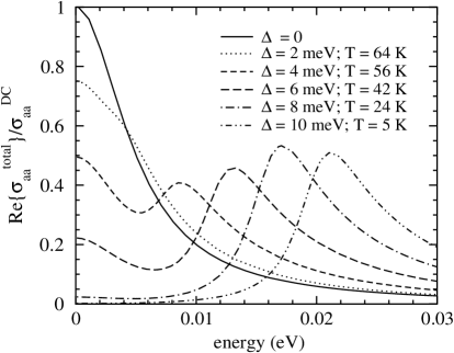
Figure 9: The development of the normalized total single-particle optical conductivity with temperature in the ordered CDW state: $\Delta(T)=\Delta_{0}\sqrt{1-T/T_{\rm CDW}}$, $\Delta_{0}=10$ meV, $T_{\rm CDW}=66$ K, $k_{\rm F}=0.5\pi/a$, $2t_{a}=0.25$ eV, $t_{b}\rightarrow 0$ and $\hbar\Gamma_{\rm intra}=\hbar\Gamma_{\rm inter}=$ 5 meV. $\sigma_{aa}^{\rm DC}$ labels the DC conductivity at $\Delta=0$.

The interplay between the self-energy and vertex-corrections terms in $\Sigma_{\underline{C}C}({\bf k},\omega)$, the correct treatment of the indirect interband optical excitations, as well as the role of the effective mass theorem in resolving all these issues will be explained elsewhere KupcicUP (12). It should be noticed here that the Landau-like function (70) gives the in-gap optical conductivity slightly different from the corresponding Lindhard-like function, as easily seen by comparing Fig. 9 with Fig. 4 reported in Ref. KupcicPB2 (15). The understanding of the difference between these two results is of general importance as well, and will be discussed in detail in Ref. KupcicUP (12).

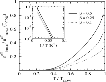
Figure 10: The temperature dependence of the normalized effective number of conduction electrons in the ordered CDW state for different values of exponent $\beta$: $\Delta_{0}=10$ meV, $T_{\rm CDW}=66$ K, $k_{\rm F}=0.5\pi/a$, $2t_{a}=0.25$ eV, $t_{b}\rightarrow 0$ and $\hbar\Gamma_{\rm intra}=\hbar\Gamma_{\rm inter}=$ 5 meV. Notice that this figure also represents the temperature behaviour of the normalized DC conductivity, since $\sigma_{aa}^{\rm DC}(T)/\sigma_{aa}^{\rm DC}(T_{\rm CDW})\approx\tilde{n}_{{\rm intra},a}^{\rm eff}(T)/\tilde{n}_{{\rm intra},a}^{\rm eff}(T_{\rm CDW})$.

V Comparison with experiments

In the simples limit, $\Sigma_{CC}({\bf k},\omega)\approx{\rm i}\Gamma_{\rm intra}$ and $\Sigma_{C\underline{C}}({\bf k},\omega)\approx{\rm i}\Gamma_{\rm inter}$, the optical conductivity of the present two-band model,

$$\sigma_{\alpha\alpha}(\omega) = \sigma^{\rm intra}_{\alpha\alpha}(\omega)+\sigma^{\rm inter}_{\alpha\alpha}(\omega),$$ (72)

is a function of the Fermi wave vector ${\bf k}_{\rm F}$, three band parameters, $t_{a}$, $t_{b}$ and $\Delta$, and two damping energies, $\hbar\Gamma_{\rm intra}$ and $\hbar\Gamma_{\rm inter}$. For $k_{{\rm F}x}\approx 0.5\pi/a$, the model illustrates optical properties of various Q1D imperfectly nested CDW systems (including both the ordered CDW state and the pseudogap effects at temperatures above the critical temperature $T_{\rm CDW}$). In this section, we shall briefly discuss a few qualitative results important to the Q1D CDW systems. First, the temperature dependence of the DC and optical conductivity in the ordered CDW state is discussed for the strictly 1D case ($t_{b}\rightarrow 0$). Then we contrast the interband conductivity found here to the oversimplified semiconducting optical conductivity usually encountered in the textbooks LRA (1, 2, 3).

V.1 DC conductivity in the ordered CDW state

The temperature dependence in $k_{\rm B}T$, $\Delta(T)$, $\Gamma_{\rm intra}(T)$ and $\Gamma_{\rm inter}(T)$ is responsible for the transfer with increasing/decreasing temperature of the optical conductivity spectra between the intraband and interband channels. This effect is particularly large in the vicinity of the metal-to-insulator phase transition. It should be noticed that, in the approximation in which $\tau({\bf k})\rightarrow\tau_{0}=1/\Gamma_{\rm intra}$ is set in Eq. ($51^{\prime}$), the temperature dependence of $\sigma_{\alpha\alpha}^{\rm DC}$ is given by the product of the effective number of conduction electrons $\tilde{n}^{\rm eff}_{{\rm intra},\alpha}(T)$ and the relaxation time $\tau_{0}(T)$. We have two adjustable parameters at any temperature, and the analysis of the DC conductivity data is thus possible only by the combination with the optical conductivity measurements. The latter method allows also the determination of the magnitude of CDW order parameter $\Delta_{0}$ and the critical exponent $\beta$ in $\Delta(T)=\Delta_{0}\big{(}1-T/T_{\rm CDW}\big{)}^{\beta}$, as well as the bond energy $t_{a}$ and the damping energy $\Gamma_{\rm inter}$.

In Figs. 9 and 10 the optical conductivity normalized to the DC conductivity at $\Delta=0$ and the temperature dependence of the DC conductivity are shown for typical values of the parameters.

V.2 Optical conductivity of a simple semiconductor

The typical result for the interband conductivity in the ordered CDW state is shown in Fig. 11 (solid and dotted curves), and compared to the data measured in the blue bronze K_0.3MoO₃ (diamonds) Degiorgi (5). Notice that the gauge-invariance factor $\hbar\omega/E_{\underline{C}C}({\bf k})$ in Eq. (70) ensures the disappearance of $\sigma_{\alpha\alpha}^{\rm inter}(0)$ at $T\rightarrow 0$, independently of the value of the phenomenologically introduced damping energy $\hbar\Gamma_{\rm inter}$. The dashed curve is the prediction of the usual optical model for semiconductors LRA (1, 2, 3), with the factor $\hbar\omega/E_{\underline{C}C}({\bf k})$ absent, which is characterized by a significant (but non-physical) contribution to $\sigma^{\rm DC}_{\alpha\alpha}$ at $T\rightarrow 0$.

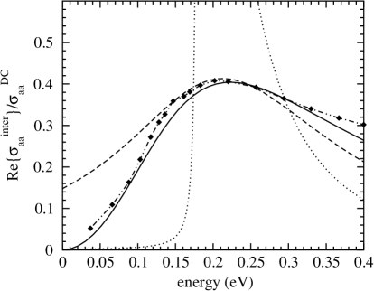
Figure 11: The interband optical conductivity (70) ($\hbar\eta\rightarrow\hbar\Gamma_{\rm inter}$), for $2t_{a}=0.4$ eV, $t_{b}\rightarrow 0$, $\Delta=0.09$ eV, $k_{\rm F}=0.5\pi/a$, $T=10$ K and $\hbar\Gamma_{\rm inter}=$ 0.3 eV (solid curve) and 1 meV (dotted curve). The dashed curve is the prediction of the usual (gauge-non-invariant) optical conductivity for semiconductors, calculated using the same band parameters, with $\hbar\Gamma_{\rm inter}=$ 0.15 eV. $\sigma^{\rm DC}_{aa}$ is the DC conductivity of the $\Delta=0$, $\hbar\Gamma_{\rm intra}=$ 0.15 eV case. The diamonds are experimental data measured in K_0.3MoO₃ at $T=10$ K Degiorgi (5).

VI Conclusion

In this article, the response of the conduction electrons in a Q1D multiband model to the transverse electromagnetic fields has been studied in presence of two scattering mechanisms. In contrast to the coherent scattering on the site-energy-dimerization potential, the impurity scattering processes give negligibly small contribution to the real part of the electron self-energy, but dominate in the relaxation processes in both the intra- and interband optical excitations. We determine the current-current correlation function, i.e. the optical conductivity of the related two-band model as a function of band filling. The transverse equation of motion approach has been used to collect the most singular contributions to the optical conductivity. It is shown that the present multiband optical analysis represents a generalization of the usual force-force correlation function method, and that in the DC limit it approaches correctly the results of Boltzmann equations, due to its gauge-invariant form. The present optical conductivity model gives the frequency and temperature dependences of the single-particle contributions to the optical conductivity spectra in the ordered CDW state which are consistent with both the experimental observation and the prediction of the longitudinal response theory. It is explained that, while the response to the longitudinal fields is associated with the direct electron-hole pair excitations, the response to the transverse electromagnetic fields can be understood in terms of the indirect (impurity-assisted) electron-hole pair excitations.

Appendix A Current and static Raman vertices

The vertex functions in the expression (29) depend on the unperturbed vertices $J^{ll}_{\alpha}({\bf k})=(e/\hbar)\partial\varepsilon_{l}({\bf k})/\partial k_{\alpha}$ and $\gamma^{ll}_{\alpha\alpha}({\bf k};2)=(m/\hbar^{2})\partial^{2}\varepsilon_{l}({\bf k})/\partial k_{\alpha}^{2}$ in the way

$$J^{LL^{\prime}}_{\alpha}({\bf k}) = \sum_{l}U_{\bf k}(l,L)U^{*}_{\bf k}(l,L^{\prime})J^{ll}_{\alpha}({\bf k}),$$

$$\gamma^{LL^{\prime}}_{\alpha\alpha}({\bf k};2) = \sum_{l}U_{\bf k}(l,L)U^{*}_{\bf k}(l,L^{\prime})\gamma^{ll}_{\alpha\alpha}({\bf k};2).$$ (73)

For the $\alpha=a$ polarization of the electromagnetic fields, the result is

$$J^{\underline{C}\underline{C},CC}_{a}({\bf k}) = \mp\big{[}u^{2}({\bf k})-v^{2}({\bf k})\big{]}J^{cc}_{a}({\bf k})$$ (74)

$$= \mp\cos\varphi({\bf k})J^{cc}_{a}({\bf k}),$$

$$J^{\underline{C}C}_{a}({\bf k}) = 2u({\bf k})v({\bf k})J^{cc}_{a}({\bf k})$$

$$= \sin\varphi({\bf k})J^{cc}_{a}({\bf k}),\hskip 85.35826pt({\rm A2}^{\prime})$$

$$\gamma^{\underline{C}\underline{C},CC}_{aa}({\bf k};2) = \mp\big{[}u^{2}({\bf k})-v^{2}({\bf k})\big{]}\gamma^{cc}_{aa}({\bf k};2)$$ (75)

$$= \mp\cos\varphi({\bf k})\gamma^{cc}_{aa}({\bf k};2).$$

Similarly, for $\alpha=b$

$$J^{\underline{C}\underline{C},CC}_{b}({\bf k})\hskip 5.69054pt=\hskip 5.69054ptJ^{cc}_{b}({\bf k}), J^{\underline{C}C}_{b}({\bf k})\hskip 5.69054pt=\hskip 5.69054pt0,$$

$$\gamma^{\underline{C}\underline{C},CC}_{bb}({\bf k};2) = \gamma^{cc}_{bb}({\bf k};2).$$ (76)

Finally, using Eqs. (18), (74) and (76) we can check the Ward identity Mahan (7) which connects the intraband current vertex $J^{LL}_{\alpha}({\bf k})$ with the electron group velocity $v^{L}_{\alpha}({\bf k})$

$$J^{LL}_{\alpha}({\bf k}) = ev^{L}_{\alpha}({\bf k})\hskip 5.69054pt=\hskip 5.69054pt\frac{e}{\hbar}\frac{\partial E_{L}({\bf k})}{\partial k_{\alpha}}.$$ (77)

References

- (1) P. A. Lee, T. M. Rice and P. W. Anderson, Solid State Commun. 14 (1974) 703.
- (2) F. Wooten, Optical Properties of Solids, Academic Press, 1972; N. W. Ashcroft and K. Sturm, Phys. Rev. B 3 (1971) 1898.
- (3) G. Grüner, Density Waves in Solids, Addison-Wesley, New York, 1994.
- (4) I. Kupčić, Physica B 322 (2002) 154.
- (5) L. Degiorgi, St. Thieme, B. Alavi, G. Grüner, R. H. Mckenzie, K. Kim and F. Levy, Physics and Chemistry of Low-Dimensional Inorganic Conductors, eds. C. Schlenker at al., Plenum Press, New York, 1996, p. 337.
- (6) K. Kim, R. H. Mckenzie and J. W. Wilkins, Phys. Rev. Lett. 71 (1993) 4015.
- (7) G. D. Mahan, Many-Particle Physics, Plenum Press, New York, 1990.
- (8) A. A. Abrikosov, L. P. Gorkov and I. E. Dzyaloshinski, Methods of Quantum Field Theory in Statistical Physics, Dover Publications, New York, 1975.
- (9) S. Doniach and E. H. Sondheimer, Green’s Functions for Solid State Physicists, W. A. Benjamin, London, 1974.
- (10) J. M. Ziman, Electrons and Phonons, Oxford University Press, London, 1972.
- (11) D. Pines and P. Noziéres, The Theory of Quantum Liquids I, Addison-Wesley, New York, 1989.
- (12) I. Kupčić and S. Barišić, to be published.
- (13) C. Kittel, Introduction to Solid State Physics, John Wiley and Sons, New York, 1996.
- (14) Notice the redundant adiabatic factor in the Fourier transformation, which is necessary in the differential treatment of the retarded correlation functions.
- (15) I. Kupčić, Physica B 344 (2004) 27.
- (16) S. L. Adler, Phys. Rev. 126 (1962) 413.
- (17) N. Wieser, Phys. Rev. 129 (1962) 63.
- (18) P. Županović, A. Bjeliš and S. Barišić, Z. Phys. B 97 (1995) 113.
- (19) J. R. Schrieffer, Theory of Superconductivity, W. A. Benjamin, New York, 1964.
- (20) D. C. Mattis and J. Bardeen, Phys. Rev. 111 (1958) 412.
- (21) M. Tinkham, Introduction to Superconductivity, Krieger, 1980.
- (22) A. A. Abrikosov and V. M. Genkin, Zh. Eksp. Teor. Fiz. 65 (1973) 842 (Sov. Phys. JETP 38 (1974) 417).
- (23) N. W. Ashcroft and N. D. Mermin, Solid State Physics, Saunders College Publishing, 1976.
- (24) In contrast to that, in the longitudinal approach, based on the charge-charge correlation functions, the long-range Coulomb interactions play the crucial role.
- (25) W. Götze and P. Wölfle, Phys. Rev. B 6 (1972) 1226.
- (26) T. Giamarchi, Phys. Rev. B 44 (1991) 2904.