Nonaffine Correlations in Random Elastic Media

Abstract

Materials characterized by spatially homogeneous elastic moduli undergo affine distortions when subjected to external stress at their boundaries, i.e., their displacements ${\mathbf{u}}({\mathbf{x}})$ from a uniform reference state grow linearly with position ${\mathbf{x}}$, and their strains are spatially constant. Many materials, including all macroscopically isotropic amorphous ones, have elastic moduli that vary randomly with position, and they necessarily undergo nonaffine distortions in response to external stress. We study general aspects of nonaffine response and correlation using analytic calculations and numerical simulations. We define nonaffine displacements ${\mathbf{u}}^{\prime}({\mathbf{x}})$ as the difference between ${\mathbf{u}}({\mathbf{x}})$ and affine displacements, and we investigate the nonaffinity correlation function ${\mathcal{G}(\mathbf{x})}=\langle[{\mathbf{u}}^{\prime}({\mathbf{x}})-{\mathbf{u}}^{\prime}(0)]^{2}\rangle$ and related functions. We introduce four model random systems with random elastic moduli induced by locally random spring constants (none of which are infinite), by random coordination number, by random stress, or by any combination of these. We show analytically and numerically that ${\mathcal{G}(\mathbf{x})}$ scales as $A|{\mathbf{x}}|^{-(d-2)}$ where the amplitude $A$ is proportional to the variance of local elastic moduli regardless of the origin of their randomness. We show that the driving force for nonaffine displacements is a spatial derivative of the random elastic constant tensor times the constant affine strain. Random stress by itself does not drive nonaffine response, though the randomness in elastic moduli it may generate does. We study models with both short and long-range correlations in random elastic moduli.

I Introduction

In the classical theory of elasticity Landau and Lifshitz (1986); Born and Huang (1954); Love (1944); Chaikin and Lubensky (1995), an elastic material is viewed as a spatially homogeneous medium characterized by a spatially constant elastic-modulus tensor $K_{ijkl}$. When such a medium is subjected to uniform stresses at its boundaries, it will undergo a homogeneous deformation with a constant strain. Such homogeneous deformations are called affine. This picture of affine strain is generally valid at length scales large compared to any characteristic inhomogeneities: displacements averaged over a sufficiently large volume are affine (at least in dimensions greater than two). It applies not only to regular periodic crystals, but also to polycrystalline materials like a typical bar of steel. At more microscopic scales, however, individual particles in an elastic medium do not necessarily follow trajectories defined by uniform strain in response to external stress: they undergo nonaffine rather than affine displacements. The only systems that are guaranteed to exhibit affine distortions at the microscopic scale are periodic solids with a single atom per unit cell. Atoms within a multi-atom unit cell of a periodic solid will in general undergo nonaffine distortions Jaric and Mohanty (1988), and atoms in random and amorphous solids will certainly undergo nonaffine distortions. Such distortions can lead to substantial corrections to the Born-Huang Born and Huang (1954) expression for macroscopic elastic moduli.

Research on fragile Durian (1995, 1997); Langer and Liu (1997); Tewari et al. (1999); Evans and Cates (2000), granular Jaeger et al. (1996); Halsey and Mehta (2002), crosslinked polymeric Rubinstein and Panyukov (1997, 2002); Glatting et al. (1997); Everaers (1998); Svaneborg et al. (2004); Sommer and Lay (2002), and biological materials Mackintosh et al. (1995); Head et al. (2003a, b, c); Wilhelm and Frey (2003), particularly in small samples, has sparked a renewed interest in the nature of nonaffine response and its ramifications. Liu and Langer Langer and Liu (1997) introduced various measures of nonaffinity, in particular the mean-square deviation from affinity of individual particles in model foams subjected to shear. Tanguy et al. Tanguy et al. (2002) in their simulation of amorphous systems of Lennard-Jones beads found substantial nonaffine response and a resultant size-dependence to the macroscopic elastic moduli. Lemaitre and Maloney Lemaitre and Maloney (2005) relate nonaffinity to a random force field induced by an initial affine response. Head et al. Head et al. (2003a, b, c) studied models of crosslinked semi-flexible rods in two-dimensions and found two types of behavior depending on the density of rods. In dense systems, the response is close to affine and is dominated by rod compression, whereas in more dilute systems, the response is strongly nonaffine and dominated by rod bending.

The recent work discussed above provides valuable insight into the nature of nonaffine response. It does not, however, provide a general framework in which to describe it. In this paper, we provide a such a framework for describing the long-wavelength properties of nonaffinity, and we verify its validity with numerical calculations of these properties on a number of zero-temperature central-force lattice models specifically designed to demonstrate our ideas. Our hope is that this framework will prove a useful tool for studying more realistic models of amorphous glasses, granular material, and jammed systems, particularly at zero temperature just above the jamming transition Liu and Nagel (1998); O’Hern et al. (2001, 2003). We are currently applying them to jammed systems Vernon et al. (2005) and to networks of semi-flexible polymers Didonna and Levine (2005).

Though nonaffinity concerns the displacement of individual particles at the microscopic scale, we show that general aspects of nonaffine response in random and amorphous systems can be described in terms of a continuum elastic model characterized by a local elastic-modulus tensor $K_{ijkl}({\mathbf{x}})$ at point ${\mathbf{x}}$, consisting of a spatially uniform average part $K_{ijkl}$ and a locally fluctuating part $\delta K_{ijkl}({\mathbf{x}})$, and possibly a local stress tensor $\tilde{\sigma}_{ij}({\mathbf{x}})$ with vanishing mean. We show that under stress leading to a macroscopic strain $\gamma_{ij}$, the random part of the elastic-modulus tensor, in conjunction with the strain $\gamma_{ij}$, acts as a source of nonaffine displacement $u^{\prime}_{i}({\mathbf{x}})$ proportional to $\partial_{j}\delta K_{ijkl}\gamma_{kl}$. For small $\delta K_{ijkl}$ and $\gamma_{ij}$, the Fourier transform of the correlation function $G_{ij}({\mathbf{x}},0)$ of the displacement ${\mathbf{u}}^{\prime}({\mathbf{x}})$ can be expressed schematically as $\gamma^{2}\Delta^{K}({\mathbf{q}})/(q^{2}K^{2})$ where $\Delta^{K}({\mathbf{q}})$ represents the Fourier transform of relevant components of the correlation function of the random part of the elastic-modulus tensor and $K$ represents the average elastic-modulus tensor. At length scales large compared to the correlation length $\xi$ of the random elastic modulus, $\Delta^{K}({\mathbf{q}})$ is a constant $\Delta^{K}$, and the nonaffinity correlation function in $d$ dimensions scales as $(\Delta^{K}/K^{2})\gamma^{2}|{\mathbf{x}}|^{-(d-2)}$, which exhibits, in particular, a logarithmic divergence in two dimensions; at length scales smaller than $\xi$, $\Delta^{K}({\mathbf{q}})\sim q^{-\phi}$, where $\phi$ can be viewed as a critical exponent, and the nonaffinity correlation function scales as $|{\mathbf{x}}|^{\phi+2-d}$ for $\phi<d$. For simplicity, we focus on zero-temperature systems. Our analytic approach is, however, easily generalized to nonzero temperature in systems with unbreakable bonds. At nonzero temperature, the dominant, long-distance behavior of nonaffinity correlation functions is the same as at zero temperature.

Our numerical studies were carried out on systems composed of sites either on regular periodic lattices or on random lattices constructed by sampling a Lennard-Jones liquid and connecting nearest-neighbor sites with unbreakable central force springs. We allowed the spring constants of the springs, their preferred lengths, or both to vary randomly. The local elastic modulus at a particular site in these models depends on the strength and length of springs connected to that site as well as on the number of springs connected to it. Thus, a periodic lattice with random spring constants and an amorphous lattice with random site coordination numbers both have a random local elastic constant. Their nonaffinity correlation function should, therefore, exhibit similar behavior, as our calculations and simulations verify. It is important to note that macroscopically isotropic systems are always amorphous and, therefore, always have a random elastic-modulus tensor and exhibit nonaffine response. For simplicity, we do not consider systems in which any spring is infinitely rigid (i.e., has an infinite spring constant). With appropriate coarse graining of $\delta K_{ijkl}({\mathbf{x}})$, however, our primary analytical results are expected to apply to this more general case.

The outline of this paper is as follows. In Sec. II, we derive familiar formulae for the elastic energy of central-force lattices and introduce our continuum model, giving special attention to the nature of random stresses. In Sec. III, we use the continuum model to calculate nonaffine response functions in different dimensions for systems with random elastic moduli with both short- and long-range correlations and with random stress tensors relative to a uniform state, and we calculate the correlation function of local rotations induced by nonaffine distortions. In Sec. IV, we present numerical results for the four model systems we consider: periodic lattices with random elastic constants without (Model A) and with (Model B) random stress, and amorphous lattices with random elastic constants without (Model C) and with (Model D) random stress. Four appendices present calculational details: Appendix A derives the independent components of the $8$th rank modulus correlator in an isotropic medium, App. B calculates the general form of the nonaffinity correlation function as a function of wavevector, App. C calculates the asymptotic forms as a function of separation ${\mathbf{x}}$ of the nonaffinity correlation function, and App. D calculates the correlation function of local vorticity.

II Models and Definitions

II.1 Notation and Model Energy

We consider model elastic networks in which particles occupy sites on periodic or random lattices in their force-free equilibrium state. Thus, particle ${\mathbf{\ell}}$ is at lattice position ${\mathbf{R}}_{{\mathbf{\ell}}0}$ in equilibrium. When the lattices are distorted, particle ${\mathbf{\ell}}$ undergoes a displacement ${\mathbf{u}}_{{\mathbf{\ell}}}$ to a new position

$${\mathbf{R}}_{{\mathbf{\ell}}}={\mathbf{R}}_{{\mathbf{\ell}}0}+{\mathbf{u}}_{{\mathbf{\ell}}}.$$ (1)

We will refer to the equilibrium lattice, with lattice positions ${\mathbf{R}}_{{\mathbf{\ell}}0}$, as the reference lattice or reference space, and the space into which the lattice is distorted via the displacements ${\mathbf{u}}_{{\mathbf{\ell}}}$ as the target space. Pairs of particles ${\mathbf{\ell}}$ and ${\mathbf{\ell}}^{\prime}$ are connected by unbreakable central-force springs on the bond $b\equiv<{\mathbf{\ell}}^{\prime},{\mathbf{\ell}}>$. The coordination number of each particle (or site) is equal to the number of particles (or sites) to which it is connected by bonds. The potential energy, $V_{b}(R_{b})$, of the spring on bond $b$ depends only on the magnitude,

$$R_{b}=|{\mathbf{R}}_{{\mathbf{\ell}}^{\prime}}-{\mathbf{R}}_{{\mathbf{\ell}}}|,$$ (2)

of the vector connecting particles ${\mathbf{\ell}}$ and ${\mathbf{\ell}}^{\prime}$. The total potential energy is thus

$$U_{T}=\sum_{b}V_{b}(R_{b})\equiv\frac{1}{2}\sum_{{\mathbf{\ell}},{\mathbf{\ell}}^{\prime}}V_{<{\mathbf{\ell}}^{\prime},{\mathbf{\ell}}>}(|{\mathbf{R}}_{{\mathbf{\ell}}^{\prime}}-{\mathbf{R}}_{{\mathbf{\ell}}}|).$$ (3)

We will consider anharmonic potentials

$$V_{b}=\frac{1}{2}k_{b}(R_{b}-R_{bR})^{2}+\frac{1}{4}g_{b}(R_{b}-R_{bR})^{4},$$ (4)

with both harmonic and quartic components, where $R_{bR}$ is the rest length of bond $b$. We assume that both $k_{b}$ and $g_{b}$ are finite. The harmonic limit is obtained when the quartic coefficient $g_{b}$ vanishes, in which case, $k_{b}$ is the harmonic spring constant.

We will only study systems in which there is an equilibrium reference state with particle positions $\{{\mathbf{R}}_{{\mathbf{\ell}}0}\}$ in which the force on each site is zero. The length $R_{b0}\equiv|{\mathbf{R}}_{{\mathbf{\ell}}^{\prime}0}-{\mathbf{R}}_{{\mathbf{\ell}}0}|$ of each bond $b$ in this configuration does not have to coincide with its rest length $R_{bR}$. As we shall see in more detail shortly, it is possible to have the total force on every site be zero but still have nonzero forces on each bond.

The potential energy of the lattice can be expanded in terms of the discrete lattice nonlinear strain Born and Huang (1954),

$$v_{b}=\frac{1}{2}(R_{b}^{2}-R_{b0}^{2})={\mathbf{R}}_{b0}\cdot\Delta{\mathbf{u}}_{b}+\frac{1}{2}(\Delta{\mathbf{u}}_{b}\cdot\Delta{\mathbf{u}}_{b})$$ (5)

relative to the reference state, where $\Delta{\mathbf{u}}_{b}={\mathbf{u}}_{{\mathbf{\ell}}^{\prime}}-{\mathbf{u}}_{\ell}$. The discrete strain variable, $v_{b}$, is by construction invariant with respect to rigid rotations of the sample, i.e., it is invariant under $R_{{\mathbf{\ell}}i}\rightarrow U_{ij}R_{{\mathbf{\ell}}j}$, where $U_{ij}$ is any ${\mathbf{\ell}}$-independent rotation matrix. To second order in $v_{b}$ in an expansion about a reference lattice with lattice sites ${\mathbf{R}}_{{\mathbf{\ell}}0}$, the potential energy is Born and Huang (1954)

$$\Delta U_{T}=\sum_{b}R_{b0}^{-1}{\tilde{F}}(b)v_{b}+\frac{1}{2}\sum_{b}R_{b0}^{-2}k(b)v_{b}^{2},$$ (6)

where ${\tilde{F}}(b)=|\tilde{\mathbf{F}}(b)|$ is the magnitude of the force,

$$\tilde{\mathbf{F}}(b)=-V_{b}^{\prime}(R_{b0}){\mathbf{R}}_{b0}/R_{b0},$$ (7)

acting on bond $b$ and

$$k(b)=V_{b0}^{\prime\prime}(R_{b0})-R_{b0}^{-1}V_{b0}^{\prime}(R_{b0})$$ (8)

is the effective spring constant of bond $b$, which reduces to $k_{b}$ when $R_{b0}=R_{bR}$. $k(b)$ is never infinite because we we assume $k_{b}$ and $g_{b}$ are finite. The equilibrium bond-length $R_{b0}$ for each bond is determined by the condition that the total force at each site ${\mathbf{\ell}}$ vanish at ${\mathbf{u}}_{{\mathbf{\ell}}}=0$:

$$F_{i}({\mathbf{\ell}})=-\left.\frac{\partial\Delta U_{T}}{\partial u_{{\mathbf{\ell}}i}}\right|_{{\mathbf{u}}_{{\mathbf{\ell}}}=0}=\sum_{{\mathbf{\ell}}^{\prime}}{\tilde{F}}_{i}(<{\mathbf{\ell}}^{\prime},{\mathbf{\ell}}>).$$ (9)

This equilibrium condition only requires that the total force on each site, arising from all of the springs attached to it, be zero Alexander (1998). It does not require that the force $\tilde{\mathbf{F}}(b)$ be equal to zero on every bond $b$.

In equilibrium, when Eq. (9) is satisfied, the part of $v_{b}$ linear in $\Delta{\mathbf{u}}_{b}$ disappears from $\Delta U_{T}$. In this case, it is customary to express $\Delta U_{T}$ to harmonic order in $\Delta{\mathbf{u}}_{b}$:

$$\Delta U_{T}^{\rm har}=\frac{1}{2}\sum_{b}[V_{b}^{\prime\prime}e_{b0i}e_{b0j}+R_{b0}^{-1}V_{b}^{\prime}(\delta_{ij}-e_{b0i}e_{b0j})]\Delta u_{bi}\Delta u_{bj},$$ (10)

where $e_{b0i}=R_{b0i}/R_{b0}$ is the unit vector directed along bond $b$. Thus the harmonic potential on each bond decomposes into a parallel part, proportional to $V_{b}^{\prime\prime}$, directed along the bond and a transverse part, proportional to $R_{b0}^{-1}V_{b}^{\prime}$, directed perpendicular to the bond. The transverse part vanishes when the force on the bond vanishes.

The harmonic energy $\Delta U_{T}^{\rm har}$ does not preserve the invariance with respect to arbitrary rotations of the full nonlinear strain energy $\Delta U_{T}$ of Eq. (6), under which

$$\Delta u_{bi}\rightarrow\Delta u^{\prime}_{bi}-(U_{ij}-\delta_{ij})R_{b0j}+U_{ij}\Delta u_{bj},$$ (11)

where $U_{ij}$ is a rotation matrix. It does, however preserve this invariance up to order $\theta^{2}$ but not order $\theta^{2}\Delta u_{b}$ and $\theta(\Delta u_{b})^{2}$, where $\theta$ is a rotation angle. For small $\bm{\theta}$,

$$\Delta{\mathbf{u}}^{\prime}_{b}=\Delta{\mathbf{u}}_{b}+\bm{\theta}\times{\mathbf{R}}_{b0}+O(\theta^{2},\theta\Delta u_{b}),$$ (12)

and ${\mathbf{e}}_{b0}\cdot\Delta{\mathbf{u}}^{\prime}_{b}={\mathbf{e}}_{b0}\cdot\Delta{\mathbf{u}}_{b}+O(\theta^{2},\theta\Delta u_{b})$. Thus, the part of the harmonic energy arising from the $k(b)$ term in Eq. (6) is invariant to the order stated above. The invariance of the force term of Eq. (6) is more subtle. Under the above transformation of Eq. (12), $(\Delta u^{\prime}_{b})^{2}=(\Delta u_{b})^{2}+2\bm{\theta}\times{\mathbf{R}}_{b}\cdot\Delta{\mathbf{u}}_{b}+(\bm{\theta}\times{\mathbf{R}}_{b})^{2}+O(\theta^{2}\Delta u_{b},\theta(\Delta u_{b})^{2})$, and it would seem that there are terms of order $\theta$, and $\theta^{2}$ in $\Delta U_{T}^{\rm har}$. These terms vanish, however, upon summation over ${\mathbf{\ell}}$ and ${\mathbf{\ell}}^{\prime}$ because of the equilibrium force condition of Eq. (9). Thus, the full $\Delta U_{T}^{\rm har}$ is invariant under rotations up to order $\theta^{2}$.

II.2 Definition of Models

We will consider the following simple models of random lattices.

Model A: Random, zero-force bonds on a periodic lattice. In this model, all sites lie on a periodic Bravais lattice with all bond lengths constant and equal to $R_{b0}$, and the rest length $R_{bR}$ of each bond is equal to $R_{b0}$. The force $\tilde{\mathbf{F}}(b)$ on each bond is zero, but the spring constant $k_{b}$ and other properties of the potential $V_{b}$ can vary from site to site. Each lattice site has the same coordination number.

Model B: Random, finite-force bonds on an originally periodic lattice. In this model, sites are originally on a regular periodic lattice, but rest bond lengths $R_{bR}$ are not equal to the initial constant bond length on the lattice. Sites in this model will relax to positions $R_{{\mathbf{\ell}}0}$ with bond lengths $R_{b0}=|{\mathbf{R}}_{{\mathbf{\ell}}^{\prime}0}-{\mathbf{R}}_{{\mathbf{\ell}}0}|$ such that the force ${\mathbf{F}}({\mathbf{\ell}})$ at each site ${\mathbf{\ell}}$ is zero but the force $\tilde{\mathbf{F}}(b)$ exerted by each bond $b$ is in general not. This model has random stresses and, as we shall see, random elastic moduli as well. The bond vectors ${\mathbf{R}}_{b0}$ and spring constant $k_{b}$ are random variables, but the coordination number of each site is not. Random stresses in an originally periodic lattice necessarily induce randomness in the elastic moduli relative to the relaxed lattices with zero force at each site.

Model C: Random, zero-force bonds on a random lattice. In this model, lattice sites are at random positions and have random coordination numbers. The equilibrium length $R_{b0}$ varies from bond to bond. The rest length $R_{bR}$ of each bond is equal to its equilibrium length so that the force $\tilde{\mathbf{F}}(b)$ of each bond is zero. This model, which is meant to describe an amorphous material, is macroscopically but not microscopically homogeneous and isotropic.

Model D: Random finite-force bonds on a random lattice. This is the most general model, and it is the one that provides the best description of glassy and random granular materials. In it, the rest lengths $R_{bR}$, the spring constants $k_{b}$, and the coordination number are all random variables. Like Model C, this model describes macroscopically isotropic and homogeneous amorphous material.

Though Models A, B, and C can be viewed as subsets of the most general model D, we find it useful to treat them as distinct models because they each isolate separate causes of randomness in the local elastic modulus or stress. One of our goals, for example, is to show analytically and numerically that the non-affinity correlations arising from structural randomness in models C and D have exactly the same form as those arising from the more controlled periodic models A and B. Another is to study the different effects of random elastic moduli and random stress.

In all of these models the random elastic-modulus tensor can in principle exhibit either short- or long-range correlations in space. To investigate the effects of such long-range correlations, we explicitly construct spring constant distributions with long-range correlations in model A. We will also find evidence of long-range correlations in model C when the reference lattice has correlated crystalline domains.

II.3 Continuum Models

In the continuum limit, when spatial variations are slow on a scale set by the lattice spacing, the equilibrium lattice positions become continuous positions ${\mathbf{x}}$ in the reference space: ${\mathbf{R}}_{{\mathbf{\ell}}0}\rightarrow{\mathbf{x}}$; and the target-space position and displacement vectors become functions of ${\mathbf{x}}$: ${\mathbf{R}}_{{\mathbf{\ell}}}\rightarrow{\mathbf{R}}({\mathbf{x}})$ and ${\mathbf{u}}_{{\mathbf{\ell}}}\rightarrow{\mathbf{u}}({\mathbf{x}})$. In this limit, the lattice strain $v_{b}$ becomes

$$v_{b}\approx R_{bi}^{0}R_{bj}^{0}u_{ij}({\mathbf{x}}),$$ (13)

where

$$u_{ij}({\mathbf{x}})=\frac{1}{2}(\partial_{i}u_{j}+\partial_{j}u_{i}+\partial_{i}{\mathbf{u}}\cdot\partial_{j}{\mathbf{u}})$$ (14)

is the full Green-Saint Venant Lagrangian nonlinear strain Love (1944); Landau and Lifshitz (1986); Chaikin and Lubensky (1995), which is invariant with respect to rigid rotations in the target space [i.e., with respect to rigid rotations of ${\mathbf{R}}({\mathbf{x}})$]. Sums over lattice sites of the form $\sum_{{\mathbf{\ell}}}S({\mathbf{\ell}})$, for any function $S({\mathbf{\ell}})$, can be replaced by integrals $\int d^{d}xS({\mathbf{x}})/v({\mathbf{x}})$ where $v({\mathbf{x}})$ is the volume of the Voronoi cell centered at position ${\mathbf{x}}={\mathbf{R}}_{{\mathbf{\ell}}0}$. The continuum energy is then

$${\cal H}=\int d^{d}x\left[\frac{1}{2}K_{ijkl}({\mathbf{x}})u_{ij}({\mathbf{x}})u_{kl}({\mathbf{x}})+{\tilde{\sigma}}_{ij}({\mathbf{x}})u_{ij}({\mathbf{x}})\right],$$ (15)

where

$${\tilde{\sigma}}_{ij}({\mathbf{x}})=-\frac{1}{2v({\mathbf{x}})}\sum_{{\mathbf{\ell}}^{\prime}}{\tilde{F}}_{i}(b)R_{b0j}|_{b=<{\mathbf{\ell}}^{\prime},{\mathbf{\ell}}>}$$ (16)

is a local symmetric stress tensor at ${\mathbf{x}}$ where the sum over ${\mathbf{\ell}}^{\prime}$ is over all bonds with one end at ${\mathbf{\ell}}$ and

$$K_{ijkl}({\mathbf{x}})=\frac{1}{2v({\mathbf{x}})}\sum_{{\mathbf{\ell}}^{\prime}}k(b)R_{b0}^{-2}R_{b0i}R_{b0j}R_{b0k}R_{b0l}|_{b=<{\mathbf{\ell}}^{\prime},{\mathbf{\ell}}>}$$ (17)

is the local elastic-modulus tensor pressure . Because it depends only on the full nonlinear strain $u_{ij}({\mathbf{x}})$, the continuum energy ${\cal H}$ of Eq. (15) is invariant with respect to rigid rotations in the target space. This is a direct result of the fact that we consider only internal forces between particles. The stress tensor ${\tilde{\sigma}}_{ij}({\mathbf{x}})$ is generated by these internal forces, and as a result, it multiplies $u_{ij}$ in ${\cal H}$. It is necessarily symmetric, and it transforms like a tensor in the reference space. (It is not, however, the second Piola-Kirchoff tensor Marsden and Hughes (1968), $\sigma_{ij}^{II}=\delta{\cal H}/\delta u_{ij}({\mathbf{x}})=K_{ijkl}u_{kl}+{\tilde{\sigma}}_{ij}$, which also transforms in this way.) External stresses, on the other hand, specify a force direction in the target space and couple to the linear part of the strain.

Since $K_{ijkl}({\mathbf{x}})$ in Eq. (17) arises from central forces on bonds, it and its average over randomness obey the Cauchy relations Love (1944); Born and Huang (1954), $K_{ijkl}({\mathbf{x}})=K_{ikjl}({\mathbf{x}})=K_{iljk}({\mathbf{x}})$, in addition to the more general symmetry relations, $K_{ijkl}({\mathbf{x}})=K_{jikl}({\mathbf{x}})=K_{ijlk}({\mathbf{x}})=K_{klij}({\mathbf{x}})$. The Cauchy relations reduce the number of independent elastic moduli in the average modulus $K_{ijkl}=\langle K_{ijkl}({\mathbf{x}})\rangle$ below the maximum number permitted for a given point-group symmetry (for the lowest symmetry, from 21 to 15). In particular, they reduce the number of independent moduli in isotropic and hexagonal systems from two to one, setting the Lamé coefficients $\lambda$ and $\mu$ equal to each other. In our analytical calculations, we will, however, treat $\lambda$ and $\mu$ as independent. The Cauchy limit is easily obtained by setting $\lambda=\mu$.

The stress tensor ${\tilde{\sigma}}_{ij}({\mathbf{x}})$ is generated entirely by internal forces on bonds. The elastic-modulus tensor $K_{ijkl}({\mathbf{x}})$ depends on the local effective spring constant $k(b)$, the length and direction of the bond vectors ${\mathbf{R}}_{b0}$, and the site coordination number; and it will be a random function of position if any of these variables are random functions of position. Thus $K_{ijkl}({\mathbf{x}})$ is a random function of position in Models A to D. The stress tensor ${\tilde{\sigma}}_{ij}({\mathbf{x}})$ is nonzero only if the bond forces are nonzero. It is thus a random function of position only in Models B and D.

We require that the continuum limit of our lattice models be in mechanical equilibrium when ${\mathbf{u}}({\mathbf{x}})=0$. This means that the linear variation of ${\cal H}$ with respect to ${\mathbf{u}}({\mathbf{x}})$ must be zero, i.e., that

$$\delta{\cal H}=\int d^{d}x{\tilde{\sigma}}_{ij}({\mathbf{x}})\partial_{j}\delta u_{i}({\mathbf{x}})=0$$ (18)

for any $\delta u_{i}({\mathbf{x}})$. $\delta u_{i}({\mathbf{x}})$ can be decomposed into a constant strain part and a part whose average strain vanishes: $\delta u_{i}({\mathbf{x}})=\delta\gamma_{ij}x_{j}+\delta{\mathbf{u}}^{\prime}({\mathbf{x}})$ where $\int d^{d}\partial_{j}\delta u^{\prime}_{i}({\mathbf{x}})=0$. Equilibrium with respect to variations in $\gamma_{ij}$ implies that the spatial average of ${\tilde{\sigma}}_{ij}$ is zero. Equilibrium with respect to $\delta{\mathbf{u}}^{\prime}({\mathbf{x}})$ implies that when ${\mathbf{x}}$ is in the interior of the sample,

$$f_{i}({\mathbf{x}})=\partial_{j}{\tilde{\sigma}}_{ij}({\mathbf{x}})=\partial_{j}{\tilde{\sigma}}_{ji}=0,$$ (19)

where ${\mathbf{f}}$ is the force density that is a vector in the target space. In addition, $\int dS_{j}{\tilde{\sigma}}_{ij}({\mathbf{x}})\delta u^{\prime}_{j}({\mathbf{x}})=0$ for any $\delta u_{j}({\mathbf{x}})$, where the integral is over the surface of the sample, implying that ${\tilde{\sigma}}_{ij}({\mathbf{x}}_{B})=0$ for points ${\mathbf{x}}_{B}$ on the surface.

Thus, we see that equilibrium conditions in the reference space impose stringent constraints on the random stress tensor ${\tilde{\sigma}}_{ij}({\mathbf{x}})$: its spatial average must be zero, its values on sample surfaces must be zero, and it must be purely transverse, i.e., it must have no longitudinal components parallel to the gradient operator. Though the linear part of $u_{ij}$ does not contribute to the stress term in ${\cal H}$, the nonlinear part still does, and ${\cal H}$ can be written as

$${\cal H} = \frac{1}{2}\int d^{d}x\left[K_{ijkl}({\mathbf{x}})u_{ij}({\mathbf{x}})u_{kl}({\mathbf{x}})\right.$$ (20)

$$\left.+{\tilde{\sigma}}_{ij}({\mathbf{x}})\partial_{i}u_{k}({\mathbf{x}})\partial_{j}u_{k}({\mathbf{x}})\right].$$

Because of the constraints on ${\tilde{\sigma}}_{ij}$, this free energy is identical to that of Eq. (15). It is invariant with respect to rotations in the target space even though it is written so that the explicit dependence on the rotationally invariant strain is not so evident rot_inv .

As we have seen, the spatial average of ${\tilde{\sigma}}_{ij}({\mathbf{x}})$ is zero; it only has a random fluctuating part in models we consider. The elastic-modulus tensor $K_{ijkl}({\mathbf{x}})$, on the other hand, has an average part and a random part with zero mean:

$$K_{ijkl}({\mathbf{x}})=K_{ijkl}+\delta K_{ijkl}({\mathbf{x}}).$$ (21)

We will view both ${\tilde{\sigma}}_{ij}({\mathbf{x}})$ and $\delta K_{ijkl}({\mathbf{x}})$ as quenched random variables with zero mean.

III Strains and nonaffinity

Consider a reference elastic body in the shape of a regular parallelepiped. When such a body is subjected to stresses that are uniform across each of its faces, it will undergo a strain deformation in which its boundary sites at positions ${\mathbf{x}}_{B}$ distort to new positions

$$R_{i}({\mathbf{x}}_{B})=\Lambda_{ij}x_{Bj},$$ (22)

where $\Lambda_{ij}$ is the deformation gradient tensor Marsden and Hughes (1968). If the medium is spatially homogeneous, then $\Lambda_{ij}\equiv\delta_{ij}+\gamma_{ij}$ determines the displacements of all points in the medium: $R_{i}({\mathbf{x}})=\Lambda_{ij}x_{j}$ or $u_{i}({\mathbf{x}})=\gamma_{ij}x_{j}$. Such a distortion is called affine. In inhomogeneous elastic media, there will be local deviations from affinity [Fig. 1] described by a displacement variable ${\mathbf{u}}^{\prime}({\mathbf{x}})$ defined via

$$R_{i}({\mathbf{x}})=\Lambda_{ij}x_{j}+u^{\prime}_{i}({\mathbf{x}})$$ (23)

or, equivalently,

$$u_{i}({\mathbf{x}}) = \gamma_{ij}x_{j}+u^{\prime}_{i}({\mathbf{x}})$$ (24)

$$u_{ij}({\mathbf{x}}) \approx \gamma_{ij}^{S}x_{j}+(\partial_{i}u^{\prime}_{j}+\partial_{j}u^{\prime}_{i}$$ (25)

$$+\gamma_{ip}\partial_{j}u^{\prime}_{p}+\gamma_{jp}\partial_{i}u^{\prime}_{p})/2,$$

where the final equation contains only terms up to linear order in ${\mathbf{u}}^{\prime}$ and where $\gamma_{ij}^{S}=(\gamma_{ij}+\gamma_{ji}+\gamma_{ik}\gamma_{jk})/2$. Since distortions at the boundary are constrained to satisfy Eq. (22), $u^{\prime}_{i}({\mathbf{x}}_{B})$ is zero for all points ${\mathbf{x}}_{B}$ on the boundary. It is often useful to consider periodic boundary conditions in which ${\mathbf{u}}^{\prime}({\mathbf{x}})$ has the same value (possibly not zero) on opposite sides of the parallelepiped. This condition implies

$$\int d^{d}x\partial_{j}u^{\prime}_{i}({\mathbf{x}})=\oint dS_{j}u^{\prime}_{i}=0.$$ (26)

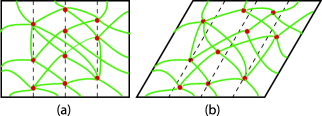
Figure 1: Sheared elastic medium with nonaffine displacements. (a) Unsheared reference state. (b) Sheared state with nonaffine displacements. Under affine distortions, points on on the vertical dotted lines in (a) would map to points on the slanted dotted lines parallel to the left and right of boundaries of the sheared sample in (b); under nonaffine distortion, they do not. [Color online]

III.1 Nonaffinity in $1d$

Figure 2: Schematic diagram of nonaffine distortion in a one-dimensional lattice with random spring constants. The top figures shows the undistorted lattice of $N$ sites with random spring constants $k_{\ell}$ and constant lattice spacing $a$. The bottom figures shows that stretched lattice with length $\gamma Na$ and random lattice spacings $a_{\ell}=\gamma+u^{\prime}_{\ell}-u^{\prime}_{\ell-1}$.

To develop quantitative measures of nonaffinity, it is useful to consider a simple one-dimensional model, which can be solved exactly. We study a one-dimensional periodic lattice, depicted in Fig. 2 with sites labelled by $\ell=0,...,N$, whose equilibrium positions are $R_{\ell 0}=a\ell$, where $a$ is the rest bond length. Harmonic springs with spring constant $k_{\ell}\equiv k+\delta k_{\ell}$ connect sites $\ell$ and $\ell-1$, where $k=(\sum_{\ell}k_{\ell})/N$ is the average spring constant and $\sum_{\ell}\delta k_{\ell}=0$. The lattice is stretched from its equilibrium length $Na$ to a new length $L=\gamma Na$. If all $k_{\ell}$’s were equal, the lattice would undergo an affine distortion with $R_{\ell}=\gamma a\ell$. When the $k_{\ell}$’s are random, sites undergo an additional nonaffine displacement $u^{\prime}_{\ell}$ so that $R_{\ell}=\gamma a\ell+u^{\prime}_{\ell}$. The energy is thus

$${\cal H}=\frac{1}{2}\sum_{\ell=1}^{N}k_{\ell}(\gamma a+u^{\prime}_{\ell}-u^{\prime}_{\ell-1})^{2}.$$ (27)

In equilibrium, the force $F_{\ell}=-\partial{\cal H}/\partial u^{\prime}_{\ell}$ on each bond is zero. The resulting equation for $u^{\prime}_{\ell}$ is

$$F_{\ell}=k_{\ell+1}(\gamma a+u^{\prime}_{\ell+1}-u^{\prime}_{\ell})-k_{\ell}(\gamma a+u^{\prime}_{\ell}-u^{\prime}_{\ell-1})=0,$$ (28)

which can be rewritten as

$$-\Delta_{+}k_{\ell}\Delta_{-}u^{\prime}_{\ell}=\gamma a\Delta_{+}\delta k_{l},$$ (29)

where $\Delta_{+}$ and $\Delta_{-}$ are difference operators defined via $\Delta_{+}A_{\ell}=A_{\ell+1}-A_{\ell}$ and $\Delta_{-}=A_{\ell}-A_{\ell-1}$ for any function $A_{\ell}$. The Fourier transforms of $\Delta_{+}$ and $\Delta_{-}$ are, respectively, $\Delta_{+}(q)=e^{iq}-1$ and $\Delta_{-}(q)=1-e^{-iq}$. Equations (28) and (29) must be supplemented with boundary conditions. We use periodic boundary conditions for which $u^{\prime}_{N}=u^{\prime}_{0}$ or equivalently

$$\sum_{\ell=1}^{N}\Delta_{-}u^{\prime}_{\ell}=0.$$ (30)

The solution to Eq. (29) can be written as the sum of a solution,

$$u_{\ell}^{I}=-(\Delta_{+}k_{\ell}\Delta_{-})^{-1}\gamma a\Delta_{+}\delta k_{\ell}=-\gamma a\Delta_{-}^{-1}\frac{\delta k_{\ell}}{k_{\ell}},$$ (31)

to the inhomogeneous equation and a solution,

$$\Delta_{+}k_{\ell}\Delta_{-}u_{\ell}^{H}=0,$$ (32)

to the homogeneous one. The latter solution is $u_{\ell}^{H}=\Delta_{-}^{-1}C/k_{\ell}$ where $C$ is an as yet undetermined constant. Adding the two solutions we obtain

$$u^{\prime}_{\ell}=\Delta_{-}^{-1}\left(-\gamma a\frac{\delta k_{\ell}}{k_{\ell}}+\frac{C}{k_{\ell}}\right),$$ (33)

which implies $\Delta_{-}u^{\prime}_{\ell}=(-\gamma a\delta k_{\ell}+C)/k_{\ell}$. The boundary condition of Eq. (30) determines $C$, and the final solution for $u^{\prime}_{\ell}$ is

$$u^{\prime}_{\ell} =-\gamma a\Delta_{-}^{-1}\frac{1}{k_{\ell}}\left[\delta k_{\ell}-(\sum k_{\ell}^{-1})^{-1}\sum k_{\ell}^{-1}\delta k_{\ell}\right]$$

$$=\gamma a\Delta_{-}^{-1}\left(\frac{k_{\ell}^{-1}}{N^{-1}\sum k_{\ell}^{-1}}-1\right)\equiv-\gamma a\Delta_{-}^{-1}S_{\ell}.$$ (34)

The quantity

$$S_{\ell}=1-\frac{(1+p_{\ell})^{-1}}{N^{-1}\sum_{1}^{\infty}(1+p_{\ell})^{-1}}$$ (35)

depends only on the ratio $p_{\ell}=\delta k_{\ell}/k$.

Equation (34) is the complete solution for $u^{\prime}_{\ell}$ for an arbitrary set of spring constants $k_{\ell}$. In our model, these spring constants are taken to be random variables, and information about the nonaffinity is best represented by correlation functions of the nonaffine displacement, averaged over the ensemble of random $k_{\ell}$’s. The simplest of these is the two-point function $G(\ell-\ell^{\prime})=\langle u^{\prime}_{\ell^{\prime}}u^{\prime}_{\ell}\rangle$, where $\langle\,\,\rangle$ represents an average over $k_{\ell}$. $G(\ell-\ell^{\prime})$ is easily calculated from Eq. (34); its Fourier transform is

$$G(q)=(\gamma a)^{2}\frac{\Delta^{S}(q)}{2(1-\cos q)},$$ (36)

where $\Delta^{S}(q)$ is the Fourier transform of $\Delta^{S}(\ell^{\prime}-\ell)=\langle S_{\ell^{\prime}}S_{\ell}\rangle$.

There are several important observations that follow from the expression Eq. (36) and that generalize to higher dimensions.

$\bullet$ $\Delta^{S}(\ell^{\prime},\ell)$ depends only on the ratios $\delta k_{\ell}/k$ and $\delta k_{\ell^{\prime}}/k$, and it increases with increasing width of the distribution of $\delta k_{\ell}$. To lowest order in averages in $\delta k_{\ell}$,

$$\Delta^{S}(\ell^{\prime},\ell) = k^{-2}[\Delta^{k}(\ell^{\prime},\ell)-N^{-1}\sum_{\ell_{1}}\Delta^{k}(\ell,\ell_{1})]$$ (37)

$$\rightarrow k^{-2}\Delta^{k}(\delta_{\ell,\ell^{\prime}}-N^{-1}),$$

where $\Delta^{k}(\ell^{\prime},\ell)=\langle\delta k_{\ell^{\prime}}\delta k_{\ell}\rangle$. The final form applies to uncorrelated distributions in which spring constants on different bonds are independent and $\langle\delta k_{\ell}\delta k_{\ell^{\prime}}\rangle=\Delta^{k}\delta_{\ell,\ell^{\prime}}$. As the width of the distribution increases, higher moments in $\delta k_{\ell}$ become important in $\Delta^{S}(\ell^{\prime},\ell)$. If we assume that the only nonvanishing fourth order moments are of the form $\Delta^{(k,4)}(\ell^{\prime},\ell)=\langle(\delta k_{\ell^{\prime}})^{2}(\delta k_{\ell})^{2}\rangle$, then the fourth-order contributions to $\Delta^{S}$ are

$$k^{4}\Delta^{(S,4)}(\ell^{\prime},\ell)$$

$$=\left(1-\frac{4}{N}+\frac{6}{N^{3}}\right)\left[\Delta^{(k,4)}(\ell^{\prime},\ell)-\frac{1}{N}\sum_{\ell_{1}}\Delta^{(k,4)}(\ell^{\prime},\ell_{1})\right]$$

$$+2\left(1-\frac{3}{N^{2}}\right)\Delta^{(k,4)}(0)\left(\delta_{\ell^{\prime},\ell}-\frac{1}{N}\right)$$

$$-\frac{1}{N}\left(2-\frac{3}{N}\right)\sum_{\ell_{1}}\Delta^{(k,4)}(\ell,\ell_{1})\left(\delta_{\ell,\ell^{\prime}}-\frac{1}{N}\right).$$ (38)

For uncorrelated distributions, $\Delta^{(k,4)}(\ell,\ell^{\prime})=\Delta^{(k,4)}\delta_{\ell,\ell^{\prime}}+(\Delta^{k})^{2}(1-\delta_{\ell,\ell^{\prime}})$. Thus, for uncorrelated distributions in the limit $N\rightarrow\infty$,

$$\Delta^{S}(q)=\left(\frac{\Delta^{k}}{k^{2}}+\frac{3\Delta^{(k,4)}-(\Delta^{k})^{2}}{k^{4}}\right)(1-\delta_{q,0})$$ (39)

to fourth order in $\delta k_{\ell}$. Note that the constraint $\sum_{\ell}\delta k_{\ell}=0$ requires $\sum_{\ell}\Delta^{S}(\ell,\ell^{\prime})=\sum_{\ell^{\prime}}\Delta^{S}(\ell,\ell^{\prime})=0$ and thus that $\Delta^{S}(q=0)=0$. This condition is imposed by the factor $1-\delta_{q,0}$ in Eq. (39), which implies that $\lim_{q\rightarrow 0}\Delta^{S}(q)\neq\Delta^{S}(q=0)=0$, i.e., $\Delta^{S}(q)$ does not approach zero as some power of $q$ as $q\rightarrow 0$.

It is easy to verify that Eq. (39) is exactly the same result that would have been obtained using only the solution [Eq. (31)] to the inhomogeneous equation for $u^{\prime}_{\ell}$ with $\delta k_{\ell}/k_{\ell}$ replaced by $\delta k_{\ell}/k_{\ell}-N^{-1}\sum_{\ell}\delta k_{\ell}/k_{\ell}$. Thus, to obtain the solution for $G(q)$ to leading order $1/N$, we can ignore the boundary condition, Eq. (30), and use the solution to the inhomogeneous equation with the constraint that $q^{2}G(q)$ be zero at $q=0$. This observation will considerably simplify our analysis of the more complicated higher-dimensional problem.

$\bullet$ If correlations in $\delta k_{\ell}$ are of finite range, then $\Delta^{S}(q)$ has a well defined $q\rightarrow 0$ limit. In this limit,

$$G(q)=(\gamma a)^{2}\frac{\Delta^{S}(0)}{q^{2}}\approx\frac{(\gamma a)^{2}}{q^{2}k^{2}}\Delta^{k}(q=0),$$ (40)

where $\Delta^{A}(0)\equiv\lim_{q\rightarrow 0}\Delta^{A}(q)$ for $A=S,k$. Thus, there is a $q^{-2}$ divergence in $G(q)$, and the spatial correlation function $\mathcal{G}(\ell^{\prime},\ell)=\langle(u_{\ell}^{\prime}-u_{\ell})^{2}\rangle$ diverges linearly in separation

$$\mathcal{G}(\ell,\ell^{\prime})\sim(\gamma a)^{2}\Delta^{S}(0)|\ell^{\prime}-\ell|\sim(\gamma a)^{2}\frac{\Delta^{k}(0)}{k^{2}}|\ell^{\prime}-\ell|.$$ (41)

$\bullet$ If correlations in $S_{\ell}$ extend out to a distance $\xi$, then $\Delta^{S}(q\xi)$ becomes a function of $q\xi$. Long-range correlations in $S_{\ell}$ will lead to long range correlations in $G(q)\sim q^{-2}\Delta^{S}(q\xi)$, and $\mathcal{G}(\ell,0)$ will grow more rapidly than $\ell$ for $1\ll\ell\ll\xi$. It is possible that this is the correlation length that diverges at the jamming point $J$ in granular media Wyart et al. (2005); Silbert et al. (2005). We will discuss this point further in Sec. III.5.

III.2 Nonaffinity for $d>1$

The nonaffinity correlation function,

$$G_{ij}({\mathbf{x}},{\mathbf{x}}^{\prime})=\langle u^{\prime}_{i}({\mathbf{x}})u^{\prime}_{j}({\mathbf{x}}^{\prime})\rangle,$$ (42)

for $d>1$ has a form very similar to that for $d=1$, except that it has more complex tensor indices. We will be primarily interested in the scalar part of this function, obtained by tracing over the indices $i$ and $j$. The Fourier transform of this function scales as

$$G({\mathbf{q}})\equiv G_{ii}({\mathbf{q}})\sim\frac{\gamma^{2}}{q^{2}}\Delta^{S}({\mathbf{q}})\sim\frac{\gamma^{2}}{q^{2}}\frac{\Delta^{K}({\mathbf{q}})}{K^{2}},$$ (43)

where $\gamma$ represents the appropriate components of the applied strain and $\Delta^{S}({\mathbf{x}},{\mathbf{x}}^{\prime})$ is in general a nonlinear function of the ratio of the fluctuating components $\delta K_{ijkl}({\mathbf{x}})$ of the elastic-modulus tensor to its uniform components $K_{ijkl}$. To lowest order in the variance, $\Delta^{S}\sim\Delta^{K}/K^{2}$ where $\Delta^{K}$ represents components of the variance of the elastic-modulus tensor and $K$ components of its average. Thus, the nonaffinity correlation function in coordinate space is proportional to $|{\mathbf{x}}|^{-(d-2)}$ in dimension $d$, or

$$\mathcal{G}({\mathbf{x}}) = \langle({\mathbf{u}}^{\prime}({\mathbf{x}})-{\mathbf{u}}^{\prime}(0))^{2}\rangle$$ (44a)

$$\sim A\ln(|{\mathbf{x}}|/B)\qquad d=2$$ (44b)

$$\sim C-D|{\mathbf{x}}|^{-1}\qquad d=3,$$ (44c)

where

$$A = \frac{1}{\pi}\gamma^{2}\Delta^{S}(0)\approx\frac{1}{\pi}\gamma^{2}\frac{\Delta^{K}(0)}{K^{2}}$$ (45a)

$$B = (\alpha\Lambda)^{-1}$$ (45b)

$$C = \gamma^{2}\Delta^{S}(0)\frac{\Lambda}{\pi^{2}}$$ (45c)

$$D = \frac{1}{\pi}\gamma^{2}\Delta^{S}(0),$$ (45d)

where $\Lambda=2\pi/a$ is the upper momentum cutoff for a spherical Brillouin zone with $a$ the short distance cutoff and $\alpha=0.8905$ is evaluated in App. C. The length $B$ depends on the spatial form and range $\xi$ of local elastic-modulus correlations. We will derive explicit forms for it shortly. In our numerical simulations, we allow the bond spring constant $k_{b}$ to be a random variable with variance $\Delta^{k}=\langle(\delta k_{b})^{2}\rangle$. Variations in $k_{b}$ in general induce changes in all of the components of $\delta K_{ijkl}$, and $\Delta^{S}$ is an average of a function of $\delta k_{b}/k$ where $k$ is the average of $k_{b}$.

In general ${\mathcal{G}(\mathbf{x})}$ also has anisotropic contributions whose angular average is zero. We will not consider these contributions in detail, but we do evaluate them analytically in App. C.

When a sample is subjected to a distortion via stresses at its boundaries, the strains can be expressed in terms of an affine strain and deviations from it. Using the expressions in Eq. (25) for these strains, we obtain the energy

$$\delta{\cal H} = \frac{1}{2}\int\{K_{ijkl}\partial_{j}u^{\prime}_{i}\partial_{l}u^{\prime}_{k}$$ (46)

$$+[\delta K_{ijkl}({\mathbf{x}})+\delta_{ik}{\tilde{\sigma}}_{jl}({\mathbf{x}})]\partial_{j}u^{\prime}_{i}\partial_{l}u^{\prime}_{k}$$

$$+2\delta K_{ijkl}({\mathbf{x}})\gamma_{kl}\partial_{j}u^{\prime}_{i}\}$$

to lowest order in $\gamma_{ij}$. Minimizing $\delta{\cal H}$ with respect to ${\mathbf{u}}^{\prime}$, we obtain

$$-\partial_{j}[K_{ijkl}+\delta K_{ijkl}({\mathbf{x}})+\delta_{ik}{\tilde{\sigma}}_{jl}({\mathbf{x}})]\partial_{l}u^{\prime}_{k}=\partial_{j}\delta K_{ijkl}({\mathbf{x}})\gamma_{kl}.$$ (47)

This equation shows that the random part of the elastic-modulus tensor times the affine strain acts as a source that drives nonaffine distortions. The random stress, which is transverse, does not drive nonaffinity; it is the continuum limit of the random force. The operator $-\partial_{j}K_{ijkl}^{T}({\mathbf{x}})\partial_{l}\delta({\mathbf{x}}-{\mathbf{x}}^{\prime})\equiv\chi_{ik}^{-1}({\mathbf{x}},{\mathbf{x}}^{\prime})$, where $K_{ijkl}^{T}({\mathbf{x}})=K_{ijkl}+\delta K_{ijkl}({\mathbf{x}})+\delta_{ik}{\tilde{\sigma}}_{jl}({\mathbf{x}})$ is the continuum limit of the dynamical matrix or Hessian discussed in Refs. Lemaitre and Maloney (2005) and Tanguy et al. (2002). The matrix $\chi_{ij}({\mathbf{x}},{\mathbf{x}}^{\prime})$ is the response $\delta u_{i}({\mathbf{x}})/\delta f_{i}({\mathbf{x}}^{\prime})$ of the displacement to an external force. The formal solution to Eq. (47) for $u^{\prime}_{i}({\mathbf{x}})$ in terms of $\delta K_{ijkl}({\mathbf{x}})$ and ${\tilde{\sigma}}_{ij}({\mathbf{x}})$ is trivially obtained by operating on both sides with $\chi_{pi}({\mathbf{x}},{\mathbf{x}}^{\prime})$:

$$u^{\prime}_{i}({\mathbf{x}})=\int d^{d}x^{\prime}\chi_{ip}({\mathbf{x}}-{\mathbf{x}}^{\prime})\partial^{\prime}_{j}\delta K_{pjkl}({\mathbf{x}}^{\prime})\gamma_{kl},$$ (48)

The random component of the elastic modulus appears both explicitly and in a hidden form in $\chi_{ip}$ in this equation.

Equation (48) is the solution to the inhomogeneous equation, Eq. (47). Solutions to the homogeneous equation should be added to Eq. (48) to ensure that the boundary condition ${\mathbf{u}}^{\prime}({\mathbf{x}}_{B})=0$ for points ${\mathbf{x}}_{B}$ on the sample boundary is met. As in the $1D$ case, however, the contribution from the homogeneous solution vanishes in the infinite volume limit and can be ignored.

To lowest order in the randomness, we replace $\chi_{ip}$ in Eq. (48) with its nonrandom counterpart, $\chi_{ip}^{0}({\mathbf{x}}-{\mathbf{x}}^{\prime})$, the harmonic elastic response function $\delta u_{i}({\mathbf{x}})/\delta f_{j}({\mathbf{x}}^{\prime})$ of a spatially uniform system with elastic-modulus tensor $K_{ijkl}$ to an external force $f_{j}({\mathbf{x}}^{\prime})$. Thus, to lowest order in $\gamma_{ij}$,

$$G_{ii^{\prime}}({\mathbf{q}})=\chi_{ip}^{0}({\mathbf{q}})\chi_{i^{\prime}p^{\prime}}^{0}(-{\mathbf{q}})q_{j}q_{j^{\prime}}\Delta_{pjkl;p^{\prime}j^{\prime}k^{\prime}l^{\prime}}^{K}({\mathbf{q}})\gamma_{kl}\gamma_{k^{\prime}l^{\prime}},$$ (49)

where

$$\Delta_{ijkl;i^{\prime}j^{\prime}k^{\prime}l^{\prime}}^{K}({\mathbf{x}},{\mathbf{x}}^{\prime})=\langle\delta K_{ijkl}({\mathbf{x}})\delta K_{i^{\prime}j^{\prime}k^{\prime}l^{\prime}}({\mathbf{x}}^{\prime})\rangle$$ (50)

is the variance of the elastic-modulus tensor, which we simply call the modulus correlator. Equation (49) contains all relevant information about nonaffine correlations to lowest order in the imposed strain. It applies to any system with random elastic moduli and stresses regardless of the symmetry of its average macroscopic state.

Our primary interest is in systems whose elastic-modulus tensor is macroscopically isotropic. In these systems, which include two-dimensional hexagonal lattices, $K_{ijkl}=\lambda\delta_{ij}\delta_{kl}+\mu(\delta_{ik}\delta_{jl}+\delta_{il}\delta_{jk})$ is characterized by only two elastic moduli, the shear modulus $\mu$ and the bulk modulus $B=\lambda+(2\mu/d)$, where $d$ is the dimension of the reference space. The Fourier transform of $\chi_{ij}^{0}({\mathbf{x}},{\mathbf{x}}^{\prime})$ in an isotropic system is

$$\chi_{ij}^{0}({\mathbf{q}})=\frac{1}{(\lambda+2\mu)q^{2}}{\hat{q}}_{i}{\hat{q}}_{j}+\frac{1}{\mu q^{2}}(\delta_{ij}-{\hat{q}}_{i}{\hat{q}}_{j}).$$ (51)

The modulus correlator is an eighth-rank tensor. At ${\mathbf{q}}=0$, it has eight independent components in an isotropic medium (See App. A) and more in media with lower symmetry, including hexagonal symmetry. As discussed above, however, all components of $\delta K_{ijkl}$ are proportional to $\delta k_{b}$.

We show in App. B that $G({\mathbf{q}})$ has the general form

$$G({\mathbf{q}})=\frac{\gamma_{xy}^{2}}{\mu^{2}q^{2}}(\Delta_{A}+\Delta_{B}{\hat{q}}_{\perp}^{2}-\Delta_{C}{\hat{q}}_{x}^{2}{\hat{q}}_{y}^{2}),$$ (52)

where ${\hat{q}}_{i}=q_{i}/q$, ${\hat{q}}_{\perp}^{2}={\hat{q}}_{x}^{2}+{\hat{q}}_{y}^{2}$ and $\Delta_{A}$, $\Delta_{B}$ and $\Delta_{C}$ are linear combinations of the independent components of $\Delta^{K}_{ijkl;i^{\prime}j^{\prime}k^{\prime}l^{\prime}}$ times a function of $\lambda/\mu$. Thus, in general ${\mathcal{G}(\mathbf{x})}$ will have anisotropic parts that depend on the direction of ${\mathbf{x}}$ in addition to an isotropic part that depends only on the magnitude of ${\mathbf{x}}$. In App. C, we derive expressions for the full form of ${\mathcal{G}(\mathbf{x})}$. Here we discuss only the isotropic part, which has the from of Eq. (44) with

$$A =\frac{\gamma_{xy}^{2}}{\pi\mu^{2}}[\Delta_{A}+\Delta_{B}-\frac{1}{8}\Delta_{C}]$$ (53)

$$B =(\alpha\Lambda)^{-1}$$ (54)

$$C =\frac{\gamma_{xy}^{2}}{\pi^{2}\mu^{2}}[\Delta_{A}+\frac{2}{3}\Delta_{B}-\frac{1}{15}\Delta_{C}]\Lambda$$ (55)

$$D =\frac{\gamma_{xy}^{2}}{2\pi\mu^{2}}[\Delta_{A}+\frac{2}{3}\Delta_{B}-\frac{1}{15}\Delta_{C}].$$ (56)

In two dimensions, the anisotropic term is proportional to $\cos 4\psi$ where $\psi$ is the angle that ${\mathbf{x}}$ makes with the $x$-axis. In the limit of large $|{\mathbf{x}}|$, the coefficient of $\cos 4\psi$ is a constant. In three dimensions, the anisotropic terms are more complicated. In both two and three dimensions, however, the average of the anisotropic terms over angles are zero.

III.3 Other Measures of Nonaffinity

The nonaffinity correlation function $G_{ij}$ (and its cousin $\cal G$) is not the only measures of nonafinity, though other measures can usually be represented in terms of it. Perhaps the simplest measure of nonaffinity is simply the mean-square fluctuation in the local value of of ${\mathbf{u}}^{\prime}({\mathbf{x}})$, which is the equal-argument limit of the trace of $G_{ij}({\mathbf{x}}^{\prime},{\mathbf{x}})$:

$$\langle[u^{\prime}({\mathbf{x}})]^{2}\rangle=G_{ii}({\mathbf{x}},{\mathbf{x}}).$$ (57)

This measure was used in Ref. Langer and Liu (1997) to measure nonaffinity in models for foams. In three dimensions, it is a number that depends on the cutoff, $a^{-1}$: $\langle[u^{\prime}({\mathbf{x}})]^{2}\rangle\sim\gamma^{2}(\Delta^{K}/K^{2})a^{-1}$; in two dimensions, it diverges logarithmically with the size of the sample $L$: $\langle[u^{\prime}({\mathbf{x}})]^{2}\rangle\sim\gamma^{2}(\Delta^{K}/K^{2})\ln(L/a)$.

References Head et al. (2003a, b, c), which investigate a two-dimensional model of crosslinked semi-flexible rods designed to describe crosslinked networks of actin and other semi-flexible biopolymers, introduce [Fig. 3] a measure based on comparing the angle $\theta\equiv\theta({\mathbf{x}}^{\prime},{\mathbf{x}})$ that the vector connecting two sites originally at ${\mathbf{x}}$ and ${\mathbf{x}}^{\prime}$ makes with some fixed axis after nonaffine distortion under shear to the angle $\theta_{0}\equiv\theta_{0}({\mathbf{x}}^{\prime})-\theta_{0}({\mathbf{x}})$ that that vector would make if the points were affinely distorted:

$$\mathcal{G}_{\theta}({\mathbf{x}}^{\prime}-{\mathbf{x}})=\langle[\theta({\mathbf{x}}^{\prime},{\mathbf{x}})-\theta_{0}({\mathbf{x}}^{\prime},{\mathbf{x}})]^{2}\rangle.$$ (58)

Under affine distortion, the vector connecting points ${\mathbf{x}}^{\prime}$ and ${\mathbf{x}}$ is $r_{i}=x^{\prime}_{i}-x_{i}+\gamma_{ij}(x^{\prime}_{j}-x_{j})$; under nonaffine distortion, the separation is ${\mathbf{r}}^{\prime}={\mathbf{r}}+{\mathbf{u}}^{\prime}({\mathbf{x}}^{\prime})-{\mathbf{u}}^{\prime}({\mathbf{x}})$. In two dimensions,

$${\mathbf{r}}\times{\mathbf{r}}^{\prime}=rr^{\prime}\sin(\theta-\theta_{0}){\mathbf{e}}_{z}={\mathbf{r}}\times[{\mathbf{u}}^{\prime}({\mathbf{x}}^{\prime})-{\mathbf{u}}^{\prime}({\mathbf{x}})],$$ (59)

where ${\mathbf{e}}_{z}$ is the unit vector along the $z$ direction perpendicular to the two-dimensional plane and $r=|{\mathbf{r}}|$. If both $\gamma$ and $|{\mathbf{u}}^{\prime}({\mathbf{x}}^{\prime})-{\mathbf{u}}^{\prime}({\mathbf{x}})|/|{\mathbf{x}}^{\prime}-{\mathbf{x}}|$ are small,

$$\theta({\mathbf{x}}^{\prime},{\mathbf{x}})-\theta_{0}({\mathbf{x}}^{\prime},{\mathbf{x}})\approx\frac{{\mathbf{e}}_{z}\cdot[({\mathbf{x}}^{\prime}-{\mathbf{x}})\times({\mathbf{u}}^{\prime}({\mathbf{x}}^{\prime})-{\mathbf{u}}^{\prime}({\mathbf{x}}))]}{|{\mathbf{x}}^{\prime}-{\mathbf{x}}|^{2}},$$ (60)

and

$$\mathcal{G}_{\theta}({\mathbf{x}})=\epsilon_{ij}\epsilon_{kl}\frac{x_{i}x_{j}}{|{\mathbf{x}}|^{4}}\mathcal{G}_{kl}({\mathbf{x}})\sim\frac{1}{|{\mathbf{x}}|^{2}}\mathcal{G}({\mathbf{x}})$$ (61)

where $\epsilon_{ij}=\epsilon_{zij}$ is the two-dimensional antisymmetric symbol, and $\mathcal{G}_{ij}({\mathbf{x}})=\langle[u^{\prime}_{i}({\mathbf{x}})-u^{\prime}_{i}(0)][u^{\prime}_{j}({\mathbf{x}})-u^{\prime}_{j}(0)]\rangle$.

Figure 3: Graphical representation of the angular measure of nonaffinity used in Ref. Head et al. (2003a). Under affine distortions, points $x_{i}$ transform to points $R_{Ai}({\mathbf{x}})=x_{i}+\gamma_{ij}x_{j}$, and the vector ${\mathbf{r}}={\mathbf{R}}_{A}({\mathbf{x}}^{\prime})-{\mathbf{R}}_{A}({\mathbf{x}})$ makes and angle $\theta_{0}({\mathbf{x}}^{\prime},{\mathbf{x}})$ with the $x$-axis. Under nonaffine distortions, points $x_{i}$ transform to $R_{i}({\mathbf{x}})=R_{Ai}({\mathbf{x}})+u^{\prime}_{i}({\mathbf{x}})$, and the vector ${\mathbf{r}}^{\prime}={\mathbf{R}}({\mathbf{x}}^{\prime})-{\mathbf{R}}({\mathbf{x}})$ makes an angle $\theta({\mathbf{x}}^{\prime},{\mathbf{x}})$ with the $x$-axis.

III.4 Generation of Random Stresses

As we have discussed, a system of particles in mechanical equilibrium can be characterized by random elastic moduli and a random local stress tensor with only transverse components. To better understand random stresses, it is useful to consider a model in which random stress is introduced in a material that is initially stress free. We begin with a system with a local elastic-modulus tensor $K_{ijkl}({\mathbf{x}})$ that can in general be random but with ${\tilde{\sigma}}_{ij}({\mathbf{x}})=0$, and to this we add a local random stress ${\overline{\sigma}}_{ij}({\mathbf{x}})$ with zero mean that couples to the rotationally invariant nonlinear strain and that has longitudinal components so that its variance in an isotropic system is

$$\Delta^{{\overline{\sigma}}}_{ijkl}=\Delta_{1}^{{\overline{\sigma}}}\delta_{ij}\delta_{kl}+\Delta_{2}^{{\overline{\sigma}}}(\delta_{ik}\delta_{jl}+\delta_{il}+\delta_{jk}).$$ (62)

For simplicity, we assume that the spatial average of ${\overline{\sigma}}_{ij}({\mathbf{x}})$ is zero. A random stress of this sort can be generated in a lattice model by making the rest bond length $R_{bR}$ a random variable in a system in which initially the rest and equilibrium bond lengths are equal. In the continuum limit, our elastic energy is thus

$$\delta{\cal H}=\int[\textstyle{\frac{1}{2}}K_{ijkl}^{\sigma}({\mathbf{x}})u_{ij}({\mathbf{x}})u_{kl}({\mathbf{x}})+{\overline{\sigma}}_{ij}({\mathbf{x}})u_{ij}({\mathbf{x}})],$$ (63)

where the superscipt $\sigma$ on $K_{ijkl}^{\sigma}$ indicates that this is an elastic modulus prior to relaxation in the presence of $\sigma_{ij}$.

Sites that were in equilibrium at positions ${\mathbf{x}}$ in the original reference space in the absence of ${\overline{\sigma}}_{ij}$ are no longer so in its presence. These sites will undergo displacements to new equilibrium sites ${\mathbf{x}}^{\prime}\equiv{\mathbf{R}}_{0}({\mathbf{x}})={\mathbf{x}}+{\mathbf{u}}_{0}({\mathbf{x}})$, which define a new reference space. Positions ${\mathbf{R}}({\mathbf{x}})$ in the target space can be expressed as displacements relative to the new reference space: ${\mathbf{R}}({\mathbf{x}}^{\prime})={\mathbf{x}}^{\prime}+{\mathbf{u}}^{\prime}({\mathbf{x}}^{\prime})$. Then, strains relative to the original reference space can be expressed as the sum of a strain relative to the new reference space and one describing the distortion of the original references space to the new one:

$$u_{ij}({\mathbf{x}}) = \frac{1}{2}\left(\frac{\partial R_{k}({\mathbf{x}})}{\partial x_{i}}\frac{\partial R_{k}({\mathbf{x}})}{\partial x_{j}}-\delta_{ij}\right)$$ (64)

$$= u_{ij}^{0}({\mathbf{x}})+\Lambda_{0ik}^{T}({\mathbf{x}}^{\prime})u^{\prime}_{kl}({\mathbf{x}}^{\prime})\Lambda_{0lj}({\mathbf{x}}^{\prime}),$$

where

$$\Lambda_{0ij}({\mathbf{x}}) = \frac{\partial R_{0i}({\mathbf{x}})}{\partial x_{j}}=\delta_{ij}+\partial_{j}u_{0i},$$ (65)

$$u_{ij}^{0} = \frac{1}{2}\left(\Lambda_{0ki}\Lambda_{0kj}-\delta_{ij}\right),$$ (66)

and

$$u^{\prime}_{ij}({\mathbf{x}}^{\prime})=(\partial^{\prime}_{i}u^{\prime}_{j}+\partial^{\prime}_{j}u^{\prime}_{i}+\partial^{\prime}_{i}u^{\prime}_{k}\partial^{\prime}_{j}u^{\prime}_{k})/2,$$ (67)

where $\partial^{\prime}_{i}\equiv\partial/\partial x^{\prime}_{i}$. Using Eq. (64) in Eq. (63), we obtain $\delta{\cal H}[{\mathbf{u}}]=\delta{\cal H}[{\mathbf{u}}_{0}]+\delta{\cal H}^{\prime}[{\mathbf{u}}^{\prime}]$, where

$$\delta{\cal H}^{\prime}=\frac{1}{2}\int d^{d}x^{\prime}[K_{ijkl}u^{\prime}_{ij}u^{\prime}_{kl}+{\tilde{\sigma}}_{jl}u^{\prime}_{ij}]$$ (68)

with

$$K_{ijkl}({\mathbf{x}}^{\prime})=(\det\Lambda_{0})^{-1}\Lambda_{0ia}\Lambda_{0jb}K_{abcd}^{\sigma}\Lambda_{0ck}^{T}\Lambda_{0dl}^{T}$$ (69)

and

$${\tilde{\sigma}}_{ij}({\mathbf{x}}^{\prime})=(\det\Lambda_{0})^{-1}\Lambda_{0ia}(K_{abcd}^{\sigma}u_{0cd}+{\overline{\sigma}}_{ab})\Lambda_{0bj}^{T},$$ (70)

where we have not displayed explicitly the dependence of $\Lambda_{0ij}$ on ${\mathbf{x}}^{\prime}$. The displacement field ${\mathbf{u}}_{0}({\mathbf{x}})$ is determined by the condition that the force density at each point in the new reference state be zero, i.e., so that $\partial^{\prime}_{j}{\tilde{\sigma}}_{ij}({\mathbf{x}}^{\prime})=0$. To linear order in displacement and ${\overline{\sigma}}_{ij}$, this condition is

$$\partial_{j}(K_{ijkl}u_{0kl}+{\overline{\sigma}}_{ij})=0,$$ (71)

where to this linearized order, we can ignore the difference between ${\mathbf{x}}$ and ${\mathbf{x}}^{\prime}$. For an initially isotropic medium, this equation can be solved for ${\mathbf{u}}_{0}$ to yield

$$u_{0i}({\mathbf{q}})=\frac{1}{\mu q^{2}}\left(\delta_{ik}-\frac{\lambda+\mu}{\lambda+2\mu}\frac{q_{i}q_{k}}{q^{2}}\right)iq_{l}{\overline{\sigma}}_{kl}.$$ (72)

To lowest order in ${\mathbf{u}}_{0}$, the elastic moduli and stress tensors in the new reference state are

$${\tilde{\sigma}}_{ij}({\mathbf{q}}) = \delta_{ik}^{T}\delta_{jl}^{T}{\overline{\sigma}}_{kl}-\frac{\lambda}{\lambda+2\mu}\delta_{ij}^{T}{\hat{q}}_{k}{\hat{q}}_{l}{\overline{\sigma}}_{kl}$$ (73)

$$\delta K_{ijkl} = 2\lambda(\delta_{ij}v_{kl}+\delta_{kl}v_{ij})$$

$$+2\mu(\delta_{ik}v_{jl}+\delta_{jl}v_{ik}+\delta_{il}v_{jk}+\delta_{jk}v_{il}),$$

where

$$v_{ij} = \frac{1}{2}\left(\Lambda_{0ik}\Lambda_{0kj}^{T}-\delta_{ij}\right)$$ (75)

$$= (\partial_{i}u_{0j}+\partial_{j}u_{0i}+\partial_{k}u_{0i}\partial_{k}u_{0j})/2$$

$$\approx (\partial_{i}u_{0j}+\partial_{j}u_{0i})/2$$

is the left Cauchy strain tensor relative to the original reference state.

Note that ${\tilde{\sigma}}_{ij}({\mathbf{x}}^{\prime})$ is transverse and random as it should be. The elastic-modulus tensor is a random variable via its dependence on $\Lambda_{0ij}({\mathbf{x}})$. Thus, a random stress added to an initially homogeneous elastic medium (with $K_{ijkl}^{0}$ nonrandom and independent of ${\mathbf{x}}$) produces both a random transverse stress and a random elastic-modulus tensor in the new relaxed reference frame. The statistical properties of $K_{ijkl}({\mathbf{x}}^{\prime})$ are determined in this model entirely by those of ${\overline{\sigma}}_{ij}({\mathbf{x}})$, and $\Delta^{K}\sim\Delta^{\overline{\sigma}}$. In general, of course, the randomness in $K_{ijkl}({\mathbf{x}}^{\prime})$ arises both from randomness in the original $K_{ijkl}^{\sigma}({\mathbf{x}})$ and ${\overline{\sigma}}_{ij}({\mathbf{x}})$.

The nonaffinity correlation function can be calculated exactly to lowest order in $\Delta^{{\overline{\sigma}}}_{1}$ and $\Delta^{{\overline{\sigma}}}_{2}$ when the initial reference state is homogeneous and nonrandom. It has exactly the same form as Eq. (43) when expressed in terms of $\Delta^{K}$. When expressed in terms of $\Delta^{{\overline{\sigma}}}_{1}$ and $\Delta^{{\overline{\sigma}}}_{2}$, it has a similar form, which in an isotopic elastic medium can be expressed as

$$G({\mathbf{q}})\sim\frac{\Delta^{{\overline{\sigma}}}_{2}\gamma^{2}}{\mu^{2}q^{2}}f({\hat{\mathbf{q}}},\lambda/\mu,\Delta^{{\overline{\sigma}}}_{1}/\Delta^{{\overline{\sigma}}}_{2}).$$ (76)

Thus, $\mathcal{G}({\mathbf{x}})$ has the same form in this model as Eq. (44).

III.5 Long-range Correlations in Elastic Moduli

Long-range correlations in random elastic moduli can significantly modify the behavior of $\mathcal{G}({\mathbf{x}})$. To illustrate this, we consider a simple scaling form for $\Delta^{K}({\mathbf{q}})$ inspired by critical phenomena:

$$\Delta^{K}({\mathbf{q}})=\xi^{\phi}g(q\xi)$$ (77)

$$\sim\begin{cases}\xi^{\phi}g_{0}[1+(q\xi)^{s}+...],&\text{for $q\xi\rightarrow 0$},\\ g_{\infty}q^{-\phi}[1+b(q\xi)^{-t}+...],&\text{as $q\xi\rightarrow\infty$},\end{cases}$$ (78)

where $\xi$ is a correlation length, $\phi$ is the dominant critical exponent, and $s$ and $t$ are corrections to scaling exponents. It is possible in principle for each of the components of $\Delta_{ijkl;i^{\prime}j^{\prime}k^{\prime}l^{\prime}}^{K}$ to be described by difference scaling lengths $\xi$ and functions $g(u)$. We will assume, however, that $\xi$ and the functional form of $g$ is the same for all components, but we will allow for the zero-argument value $g_{0}$ to vary. $G({\mathbf{q}})$ is thus given by Eq. (52) with $\Delta_{A}$, $\Delta_{B}$, and $\Delta_{C}$ replaced by $\Delta_{A}({\mathbf{q}})$, $\Delta_{B}({\mathbf{q}})$, and $\Delta_{C}({\mathbf{q}})$ with scaling forms given by Eq. (77). In this case, ${\mathcal{G}(\mathbf{x})}$ can be written as $(\gamma_{xy}^{2}/\mu^{2})\mathcal{F}({\mathbf{x}})$ with $\mathcal{F}({\mathbf{x}})={\mathcal{F}}_{A}({\mathbf{x}})+{\mathcal{F}}_{B}({\mathbf{x}})-{\mathcal{F}}_{C}({\mathbf{x}})$, where

$${\mathcal{F}}_{\alpha}({\mathbf{x}})=2\xi^{\phi}\int\frac{d^{d}q}{(2\pi)^{d}}f_{\alpha}({\mathbf{q}})g_{\alpha}(q\xi)\frac{1}{q^{2}}(1-e^{i{\mathbf{q}}\cdot{\mathbf{x}}}),$$ (79)

with $f_{A}=1$, $f_{B}({\mathbf{q}})={\hat{q}}_{\perp}^{2}$, and $f_{C}({\mathbf{q}})={\hat{q}}_{x}^{2}{\hat{q}}_{y}^{2}$. There are two important observations to make about the functions ${\mathcal{F}}_{\alpha}$. First, for $q\xi\ll 1$, $g(q\xi)$ can be replaced by its zero $q$ limit, $g_{0}$. Thus, as long as $\xi$ is not infinite, the asymptotic behavior of $\mathcal{G}({\mathbf{x}})$ for $|{\mathbf{x}}|\gg\xi$ is identical to those of Eq. (44) but with amplitudes that increase as $\xi^{\phi}$. Second, when $\xi\rightarrow\infty$, the $q^{(d-3-\phi)}$ behavior of the integrand leads to modified power-law behavior in $|{\mathbf{x}}|$ for $a\ll x\ll\xi$, where $a=2\pi/\Lambda$ is the short distance cutoff, depending on dimension.

In two dimensions, which is the focus of most of our simulations, the isotropic part of ${\mathcal{F}}$ is

$${\cal F}_{I}({\mathbf{x}})=\frac{\xi^{\phi}}{\pi}\int_{0}^{\Lambda}\frac{dq}{q}g(q\xi)[1-J_{0}(q|{\mathbf{x}}|)],$$ (80)

where $g(y)=g_{A}(y)+g_{B}(y)-\frac{1}{8}g_{C}(y)$ and $J_{0}(y)$ is the zeroth order Bessel function. In the limit $|{\mathbf{x}}|\gg\xi$,

$${\mathcal{F}}_{I}({\mathbf{x}})\sim\frac{1}{\pi}g_{0}\xi^{\phi}\ln\frac{\beta(\Lambda\xi,\phi)}{\xi}|{\mathbf{x}}|,$$ (81)

where $\beta(\Lambda\xi,\phi)$ is evaluated in Appendix C. The behavior of ${\mathcal{F}}_{I}({\mathbf{x}})$ when $\Lambda^{-1}\ll|{\mathbf{x}}|\ll\xi$ depends on the value of $\phi$

$${\mathcal{F}}_{I}({\mathbf{x}})\sim\begin{cases}\frac{1}{\pi}g_{\infty}|{\mathbf{x}}|^{\phi}\mathcal{A}_{2}(\phi),&\text{if $\phi<2$},\\ \frac{1}{4\pi}g_{\infty}|{\mathbf{x}}|^{2}\ln(\nu\xi/|{\mathbf{x}}|),&\text{if $\phi=2$},\\ \frac{1}{4\pi}g_{\infty}|{\mathbf{x}}|^{2}\xi^{\phi-2}\mathcal{C}_{2}(\phi),&\text{if $\phi>2$}.\end{cases}$$ (82)

The quantities $\mathcal{A}_{2}(\phi)$, $\mathcal{C}_{2}(\phi)$, and $\nu$ are evaluated in Appendix C.

The function $g(u)$ can have any form provided its large- and small-$u$ limits are given by Eq. (77). A useful model form to consider, of course, is the simple Lorentzian for which $\phi=2$ and

$$g(u)=\frac{g_{0}}{1+u^{2}}.$$ (83)

For the purposes of illustration, in Fig. 4 we plot ${\cal F}_{i}(|{\mathbf{x}}|)$ for a family of functions parameterized by the exponent $\phi$:

$$g(u)=\frac{g_{0}(\phi)}{(1+u^{2})^{\phi/2}}.$$ (84)

these curves clearly show the crossover from $|{\mathbf{x}}|^{\phi}$ behavior for $\Lambda^{-1}\ll|{\mathbf{x}}|\ll\xi$ to the characteristic log behavior for $|{\mathbf{x}}|\gg\xi$. The correlation length $\xi$ and the amplitude $g_{0}(\phi)$ were set so that the large ${\mathbf{x}}$ log behavior is the same for every $\phi$. For this family of crossover functions, the value of $|{\mathbf{x}}|$ at which ${\cal F}(|{\mathbf{x}}|)$ crosses over from $|{\mathbf{x}}|^{\phi}$ to logarithmic behavior increases with decreasing $\phi$, and curves with smaller $\phi$ systematically lie above those with large $\phi$.

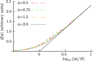
Figure 4: The function ${\cal G}(|{\mathbf{x}}|)$ in two dimensions for fixed $\gamma$ and $K$ for systems with long-range correlations in $\Delta^{K}$ defined by Eqs. (80) and (84) for different exponents $\phi$. The amplitudes and correlation lengths $\xi$ for each $\phi$ are normalized so that all curves have the same values of $B=\xi/\beta(\Lambda\xi,\phi)$ and coefficients of $\ln|{\mathbf{x}}|/B$ at large $|{\mathbf{x}}|/B$. The curve for $\phi=2$ corresponds to Lorentzian correlations [Eq. (83)]. [Color online]

The limiting forms for ${\cal F}_{I}(|{\mathbf{x}}|)$ in one and three dimensions are given in App. C.

III.6 Rotational Correlations

The nonaffine displacements generated in random elastic media by external strains contain rotational as well as irrotational components as is evident from Fig. (5). The local nonaffine rotation angle is $\omega_{k}({\mathbf{x}})=\frac{1}{2}\epsilon_{ijk}\partial_{j}u^{\prime}_{k}$, where $\epsilon_{ijk}$ is the anti-symmetric Levi-Civita tensor, and rotational correlations are measured by the correlation function $G_{\omega_{i}\omega_{j}}({\mathbf{x}})=\langle\omega_{i}({\mathbf{x}})\omega_{j}(0)\rangle$. In two dimensions, there is only one angle $\omega({\mathbf{x}})=\frac{1}{2}\epsilon_{ri}\partial_{r}u_{i}$, where $\epsilon_{ri}\equiv\epsilon_{zri}$. The Fourier transform of the correlation function $G_{\omega}=\langle\omega({\mathbf{x}})\omega(0)\rangle$ will then scale as $\gamma^{2}\Delta^{K}/\mu^{2}$, approaching a constant rather than diverging as ${\mathbf{q}}\rightarrow 0$. We show in App. D that

$$G_{\omega}({\mathbf{q}})=\frac{\gamma_{xy}^{2}}{\mu^{2}}[\Delta_{A}^{\omega}(q)-\Delta^{\omega}_{C}(q){\hat{q}}_{x}^{2}{\hat{q}}_{y}^{2}]$$ (85)

in two dimensions, where $\Delta_{A}^{\omega}(q)$ and $\Delta_{C}^{\omega}$ are linear combinations of the independent components of $\Delta^{K}_{ijkl;i^{\prime}j^{\prime}k^{\prime}l^{\prime}}$. Thus, the rotation correlation function contains direct information about elastic-modulus correlations. If these correlations are short range, and there is no $q$ dependence in either $\Delta_{A}^{\omega}(q)$ or $\Delta_{C}^{\omega}$, the spatial correlation function has an isotropic short-range part and an anisotropic power-law part:

$$G_{\omega}({\mathbf{x}})=\frac{\gamma_{xy}^{2}}{\mu^{2}}\left[\Delta_{A}^{\omega}\delta({\mathbf{x}})-\Delta_{C}^{\omega}\left(16\frac{x^{2}y^{2}}{|{\mathbf{x}}|^{6}}-\frac{2}{|{\mathbf{x}}|^{2}}\right)\right].$$ (86)

If there are long-range correlations in the elastic moduli with the Lorentzian form of Eq. (83), then

$$G_{\omega}({\mathbf{x}}) = \frac{\gamma_{xy}^{2}}{2\pi\mu^{2}}\Bigl{[}\left({\tilde{\Delta}}_{A}^{\omega}-\frac{1}{8}\Delta_{C}^{\omega}\right)K_{0}(|{\mathbf{x}}|/\xi)$$

$$+\frac{1}{8}\cos 4\psi{\tilde{\Delta}}_{C}^{\omega}\left(-\frac{48\xi^{4}}{|{\mathbf{x}}|^{4}}+\frac{4\xi^{2}}{|{\mathbf{x}}|^{2}}+K_{4}(|{\mathbf{x}}|/\xi)\right)\Bigr{]},$$

where $K_{n}(y)$ is the Bessel function of imaginary argument. The $\cos 4\psi$ behavior is for isotropic systems. There will be $\cos 6\psi$ and higher order terms present in a hexagonal lattice. In Sec. IV, we verify in numerical simulations the exponential decay of the isotropic part of $G_{\omega}(|{\mathbf{x}}|)$ in Model A with long-range correlations in spring constants and the $|{\mathbf{x}}|^{-2}$ behavior of the $\cos 4\psi$ part of $G_{\omega}(|{\mathbf{x}}|)$ in Model C, which is isotropic.

Figure 5: This figure shows the direction of nonaffine displacements resulting from a shear in the $xy$-plane displayed as arrows on the original reference lattice. Note the vortex-like patterns.

IV Numerical Minimizations

To further our understanding of nonaffinity in random lattices and to verify our analytic predictions about them, we carried out a series of numerical studies on models A-D described in Sec. II.1. To carry out these studies, we began with an initial lattice – a periodic hexagonal or FCC lattice for models A and B and a randomly tesallated lattice for models C and D. We assigned spring potentials $V_{b}(R_{b})$ and rest bond lengths $R_{bR}$ to each bond. To study nonaffinity, we subjected lattices to shear and then numerically determined the minimum-energy positions of all sites subject to periodic boundary condition. The elastic energy of the lattice was linearized about the affine shear state. Interestingly, in this linearization the value of the imposed shear, $\gamma$, factored out of our calculation, so that ${\bf u}^{\prime}({\bf x})$ was linear in $\gamma$ and thus ${\mathcal{G}(\mathbf{x})}$ was automatically quadratic in $\gamma$. We present below the procedures and results for each model.

IV.1 Model A

In this model, the initial reference lattice is periodic, and the rest bond length $R_{bR}$ is equal to the equilibrium lattice parameter $R_{b0}$ for every bond, which we set equal to one. Each bond is assigned an anharmonic potential

$$V_{b}(R_{b})=\frac{1}{2}k_{b}(\delta R_{b}^{2}+\delta R_{b}^{4}),$$ (88)

where $\delta R_{R}=R_{b}-R_{b0}\equiv R_{b}-1$ and the spring constant $k_{b}$ is a random variable. We chose $k_{b}=1+\delta k_{b}$ where $\delta k_{b}$ is a random variable with zero mean lying between $-\delta{\overline{k}}$ and $+\delta{\overline{k}}$ with $\delta{\overline{k}}<1$.

IV.1.1 Independent bonds on hexagonal and FCC lattice

In the simplest versions of model A, the spring constant $k_{b}$ is an independent random variable on each bond of a two-dimensional hexagonal or a three-dimensional FCC lattice. We assign each bond a random value of $\delta k_{b}$ chosen from a flat distribution lying between $-\delta{\overline{k}}$ and $+\delta{\overline{k}}$. Randomly distributed spring constants give rise to random local elastic moduli as defined by Eq. (17). We verified that the distribution of the values of the local shear modulus $K_{xyxy}$ on a hexagonal lattice for different $\delta{\overline{k}}$ was well fit by a Gaussian function with width linearly proportional to $\delta{\overline{k}}$.

The nonaffinity correlation function ${\mathcal{G}(\mathbf{x})}=\langle\left|{\bf u}^{\prime}({\mathbf{x}})-{\bf u}^{\prime}(0)\right|^{2}\rangle$ [Eq. (44)] measured on the numerically relaxed lattices is shown in Fig. 6(a). The averages were calculated by summing the differences in deviation for every pair of nodes on the lattice and binning according to the nodes’ separation in the undeformed (reference) state. Note that this process automatically averages over angle, so it produces only the isotropic part of ${\mathcal{G}(\mathbf{x})}$. The separation between nodes was taken as the least distance between the nodes across any periodic boundaries. The curves were well fit by the $A\ln({\left|{\mathbf{x}}\right|}/B)$ dependence on ${\left|{\mathbf{x}}\right|}$ predicted by Eq. (44b). The excellent data collapse achieved by plotting the rescaled function ${\mathcal{G}(\mathbf{x})}/(\gamma\delta{\overline{k}})^{2}$ demonstrates the quadratic dependence of the amplitude $A$ on $\delta{\overline{k}}$. Figure 7 shows the quadratic plus quartic dependence of the amplitude $A$ on and $\delta{\overline{k}}$ at larger values. It is worth noting that while all correlation functions were independently fit with a two-parameter function $A\ln({\left|{\mathbf{x}}\right|}/B)$, the optimal values of $B$ in all cases fell within $10\%$ of one another.

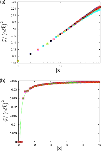
Figure 6: The nonaffinity correlation function ${\mathcal{G}(\mathbf{x})}/(\gamma\delta{\overline{k}})^{2}$ for sheared model-A lattice: (a) ${\mathcal{G}(\mathbf{x})}/(\gamma\delta{\overline{k}})^{2}$ versus ${\left|{\mathbf{x}}\right|}$ for a $2$D hexagonal lattice sheared to $0.1\%$ for values $\delta{\overline{k}}=0.01n$ for $n=1,...,10$ of the variation in local spring constant. (b) ${\mathcal{G}(\mathbf{x})}/(\delta{\overline{k}})^{2}$ versus ${\left|{\mathbf{x}}\right|}$ for a $3$D FCC lattice sheared to $0.1\%$ for several different values $\delta{\overline{k}}=0.01n$ for $n=1,...,10$. The data is fit to a function $C-D/{\left|{\mathbf{x}}\right|}$. All lengths are in units of the lattice spacing. [Color online]

Figure 7: (a)The prefactor A of the fits in plots of Fig. 6(a) as a function of $\delta{\overline{k}}$. The dotted curve is a fit to a quartic $g(\delta{\overline{k}})^{2}+h(\delta{\overline{k}})^{4}$ as suggested by Eq. (39). The inset shows data up to $\delta{\overline{k}}=0.1$ and a quadratic fit.

Figure 6(b) displays ${\mathcal{G}(\mathbf{x})}/(\delta{\overline{k}})^{2}$ on an FCC lattice as a function of ${\left|{\mathbf{x}}\right|}$ for different $\delta{\overline{k}}$ for $\gamma=0.1\%$ fit to the function $C-D/{\left|{\mathbf{x}}\right|}$ predicted by Eq. (44). The data collapse verifies the expected dependence of $C$ on $(\delta{\overline{k}})^{2}$.

IV.1.2 Correlated random bonds on an hexagonal lattice

As discussed in Sec. III.5, random lattices can exhibit long-range correlations, characterized by a correlation length $\xi$, in local elastic moduli that can significantly modify the behavior of nonaffinity correlation functions at distances less than $\xi$. To verify the prediction of Sec. III.4, we numerically constructed hexagonal lattices with long-range correlations in bond spring constants. To do this, we set $k_{b}=1+\delta k_{b}$ where $\delta k_{b}$ was set equal to a small, randomly generated scalar field with proper spatial correlations. This scalar field was created by taking the reverse Fourier transform of the function $\exp(i\phi_{r})/\sqrt{q^{2}+\xi^{-2}}$, where $\xi$ is a variable decay length and $\phi_{r}$ is a random complex phase. The scalar field in these simulations was normalized to have constant mean squared value and peak values of $\pm 0.1$, so that the variation to the local spring constants was at most $10\%$. This method of generation yields a clean exponential decay in the two-point correlation function $\Delta^{K}({\mathbf{x}},0)\equiv\langle\delta K_{xyxy}({\mathbf{x}})\delta K_{xyxy}(0)\rangle$ which persists for separations up to three times the correlation length. Figure 8 shows the two-point correlation function $\Delta^{K}({\mathbf{x}},0)$ as a function of separation. The region of exponential correlation was followed by a small region of anti-correlation, which is not pictured. By construction, the distributions of the local shear elastic modulus $K_{xyxy}$ were essentially constant, independent of $\xi$; thus $\Delta^{K}(0,0)$ is equal for all curves in Fig. 8.

According to Eq. (111), the growth of the correlation function ${\mathcal{G}(\mathbf{x})}$ for large $\left|{\mathbf{x}}\right|$ is logarithmic with prefactor proportional to $g_{0}\xi^{\phi}$, where $\phi=2$ for the Lorentzian case we are now considering. The quantity $g_{0}\xi^{\phi}$ is equivalent to $\Delta^{K}({\mathbf{q}}\!=\!0)$, but this quantity is difficult to measure numerically. However, $g_{0}$ can also be expressed in terms of the coordinate space correlation $\Delta^{K}({\mathbf{x}}\!=\!0)$. The latter quantity is easily measured by averaging $\left<\left(\delta K_{xyxy}({\mathbf{x}})\right)^{2}\right>$ over all nodes. For the form of the correlation function $g(u)$ given in Eq. (84),

$$\Delta^{K}({\mathbf{x}}\!=\!0)\sim g_{0}\xi^{\phi-2}\begin{cases}\frac{1}{\phi-2}\left(1-\left(1+\left(\Lambda\xi\right)^{2}\right)^{1-\frac{\phi}{2}}\right)&\phi\neq 2,\\ \frac{1}{2}\ln\left(1+\left(\Lambda\xi\right)^{2}\right)&\phi=2.\end{cases}$$ (89)

In the limit $\xi\Lambda\gg 1$, $g_{0}\sim\Delta^{K}({\mathbf{x}}\!=\!0)$ and the large separation form of the correlation function ${\mathcal{G}(\mathbf{x})}$ is logarithmic with prefactor $\gamma^{2}\Delta^{K}({\mathbf{x}}\!=\!0)\xi^{\phi}/\mu^{2}$.

We have already established that for this set of simulations, $\Delta^{K}({\mathbf{x}}\!=\!0)/\mu^{2}$ is a constant, independent of $\xi$ [see Fig.8]. In Fig. 9, we plot ${\mathcal{G}(\mathbf{x})}/\xi^{2}$ versus ${\left|{\mathbf{x}}\right|}/\xi$ for different values of $\xi$. We also plot the function $\mathcal{F}({\left|{\mathbf{x}}\right|})$ calculated from Eq. (80) with a Lorentzian $g(y)$ [Eq. (83)]. The agreement between the numerical and analytical results is excellent with both showing ${\left|{\mathbf{x}}\right|}^{2}$ behavior for ${\left|{\mathbf{x}}\right|}<\xi$ and $\ln{\left|{\mathbf{x}}\right|}$ behavior for ${\left|{\mathbf{x}}\right|}>\xi$. In Fig. 10 we plot the vorticity correlation function $G_{\omega}$ versus separation rescaled by the correlation length, ${\left|{\mathbf{x}}\right|}/\xi$. The vorticity correlation function decreases exponentially away from zero separation with a decay length $\sim 1.1\times\xi$; our framework predicted decay with an exponent of $\xi$ exactly. The slight discrepency between theory and simulation is not understood.

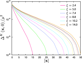
Figure 8: The two point correlation function $\Delta^{K}({\mathbf{x}}\!=\!0)=\langle\delta K_{xyxy}({\mathbf{x}})\delta K_{xyxy}(0)\rangle$ produced by random spring constants drawn from an exponentially correlated random scalar field. The exponential decay is evident. [Color online]

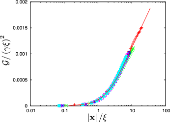
Figure 9: Plot of ${\mathcal{G}(\mathbf{x})}/\xi^{2}$ versus ${\left|{\mathbf{x}}\right|}/\xi$ for different $\xi$ from (points) numerical minimizations and (solid line) the analytical expression of Eq. (80) with a Lorentzian $g(y)$. [Color online]

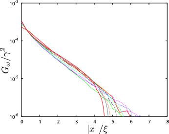
Figure 10: Plot of the vorticity correlation $G_{\omega}$ versus ${\left|{\mathbf{x}}\right|}/\xi$ for several different $\xi$ for lattices with Lorentzian spatial correlations in $\delta k_{b}$. [Color online]

IV.2 Model B: Internal stresses

In this model, random stresses are introduced in a periodic lattice via a random distribution of rest bond lengths. We study hexagonal lattices in which the rest lengths of the bonds are multiplied by a factor $(1+\beta_{b})$ where $\beta_{b}$ is chosen randomly from a flat distribution lying between $-\beta$ and $\beta$ with $\beta<0.1$. Once again, the spring constants are set to $k_{b}=1+\delta k_{b}$, with $\delta k_{b}$ chosen randomly from a flat distribution lying between $-\delta{\overline{k}}$ and $+\delta{\overline{k}}$. After specifying the rest length of each bond, we numerically determined the equilibrium state of this random lattice with zero applied stress by minimizing the rest energy over lattice positions and the size of the simulation box (for a system of 40,000 particles, the minimization over box size was only a fraction of a percent). The resulting equilibrium configuration has zero net force on each node. This relaxed state constitutes the reference state of our random system with lattice positions ${\mathbf{R}}_{{\mathbf{\ell}}0}={\mathbf{x}}$.

The original lattice before relaxation is characterized by random stresses ${\overline{\sigma}}_{ij}$, which can be calculated from Eq. (16),

$${\overline{\sigma}}_{ij}({\mathbf{\ell}})=\frac{1}{2v}\sum_{{\mathbf{\ell}}^{\prime}}R_{bIi}R_{bIj}k_{b}\delta R_{b}/a,$$ (90)

where ${\mathbf{R}}_{bI}$ is the bond vector of length $a$ (independent of $b$) for bond $b$ in the initial undistorted hexagonal lattice and $\delta R_{b}=a-R_{bR}=\beta_{b}a$. The average over of ${\overline{\sigma}}_{ij}$ over $\beta_{b}$ is zero: $\langle{\overline{\sigma}}_{ij}\rangle_{b}=0$, and its variance is

$$\langle{\overline{\sigma}}_{ij}({\mathbf{\ell}}){\overline{\sigma}}_{kl}({\mathbf{\ell}})\rangle_{b}=\frac{\beta^{2}}{27}(1+\frac{(\delta\overline{k})^{2}}{3})(\delta_{ij}\delta_{kl}+\delta_{ik}\delta_{jl}+\delta_{il}\delta_{jk}).$$ (91)

As discussed in Sec. III.4, randomness in ${\overline{\sigma}}_{ij}$ generates a random elastic moduli in the relaxed reference lattice. Figure 11 shows how the random stress broadens the distribution of local elastic moduli. For lattices with $\delta\bar{k}=0$, $\sqrt{\Delta^{K}({\mathbf{x}}\!=\!0)}$ is linearly proportional to $\beta$ as predicted by Eqs. (72) to (75).

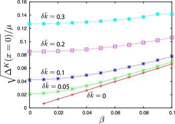
Figure 11: The variance of the local shear modulus versus $\beta$ for several different $\delta\bar{k}$. [Color online]

After constructing the relaxed state, we sheared it in the $xy$ plane as before and measured the nonaffinity correlation function. The measurements were well fit by the functional form ${\mathcal{G}(\mathbf{x})}\sim A\ln({\left|{\mathbf{x}}\right|}/B)$. Figure 12 shows that for $\delta\bar{k}=0$ the measured ratio $A/(\gamma^{2}\Delta^{K}({\mathbf{x}}\!=\!0)/\mu^{2})$ is nearly independent of $\beta$, as predicted in Section III.4. For $\delta\bar{k}>0$, the ratio $A/(\gamma^{2}\Delta^{K}({\mathbf{x}}\!=\!0)/\mu^{2})$ is $\sim 20\%$ lower at small $\beta$, but asymptotes to the $\delta\bar{k}=0$ value as $\beta$ increases, approaching the asymptote more quickly for smaller $\delta\bar{k}$. The difference in $A/(\gamma^{2}\Delta^{K}({\mathbf{x}}\!=\!0)/\mu^{2})$ between stressed and stress-free lattices is most likely a higher order effect due to the breaking of hexagonal symmetry as $\beta$ is increased.

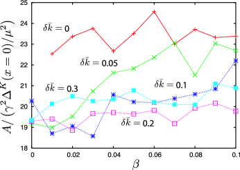
Figure 12: $A/(\gamma^{2}\Delta^{K}({\mathbf{x}}\!=\!0)/\mu^{2})$ versus $\beta$ for several different $\delta\bar{k}$. [Color online]

IV.3 Model C: Random lattice

In this model, the initial reference lattice is geometrically random. The rest bond length $R_{bR}$ is equal to the equilibrium lattice parameter $R_{b0}$ for every bond, so that the reference state is stress free. Our method of generating reference lattices of varying randomness is detailed below. Each bond is assigned the anharmonic potential of Eq. (88), where the spring constant $k_{b}(R_{b})=k_{0}/R_{b}$ is a constant per unit length of the rest bond length.

We use the approach followed in Chung et al. (2002) to generate networks with a tunable degree of randomness. We begin by simulating a $2$-dimensional gas of $40000$ point particles interacting through a Lennard-Jones potential. The procedure outlined in Berendsen et al. (1984) is used to equilibrate the gas at a prescribed temperature and pressure, with periodic boundary conditions. The gas is equilibrated for $10000$ time steps, after which the particle configurations are sampled every $1000$ time steps. In this manner we obtain $40$ uncorrelated configurations of the gas at thirteen different temperature-pressure combinations, with $T=8.0$ and $P=0.025$, $0.05$, $0.1$, $0.2$, $0.25$, $0.3$, $0.35$, $0.4$, $0.5$ $0.6$, $0.7$, $0.8$, and $1.0$, all in units of the Lennard-Jones potential.

Figure 13: Section of a random lattice created by triangulating a snapshot of a Lennard-Jones gas with $T=8.0$ and $P=0.05$.

We use the particle positions from the snapshots of the equilibrated gas as the positions of nodes in our random lattice. Each sampled configuration is rescaled to have a box length of $1$ on each side. The point configurations are then tesselated using the Delaunay triangulation, which places a bond between each node and its nearest neighbors. The Delaunay triangulation produces networks with an average of $6$ bonds per node. A resulting lattice is pictured in Fig. 13.

The randomness in local elastic moduli as calculated from Eq. (17) is proportional to the distribution of bond lengths and bonds per node. In principle, as we take the equilibrium gas pressure to zero, the distribution of bond lengths will become completely random. Conversely, as we increase the pressure past a critical point the simulated gas begins to crystalize, forming spatial domains of hexagonal order separated by grain boundaries. This transition should be marked by a growth in the two-point correlation of local shear moduli. We fit the non-affinity correlation data for a broad range of pressures which cross this transition and compare it to the framework developed in previous sections. We used Eq. (17) to calculate $\Delta^{K}({\mathbf{x}}\!=\!0)/\mu^{2}$ for each ensemble of random lattices, while the crystalline correlation length is fit as an unknown.

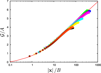
Figure 14: ${\mathcal{G}(\mathbf{x})}$ vs ${\left|{\mathbf{x}}\right|}$ for lattices with varying degrees of geometrical randomness, scaled to have the same asymptotic form for large ${\left|{\mathbf{x}}\right|}$. The solid line is a fit Eq. (80) using $g(u)$ of Eq. (84) with $\phi=0.4$. [Color online]

The lattice is sheared by $0.1\%$ and the energy is minimized as a function of node position as before. Figure 14 shows the displacement correlation function ${\mathcal{G}(\mathbf{x})}$ as a function of separation ${\left|{\mathbf{x}}\right|}$ for lattices with different degrees of randomness. This correlation function shows the same logarithmic growth at large ${\left|{\mathbf{x}}\right|}$ as it does in the random spring constant lattices from the last section.

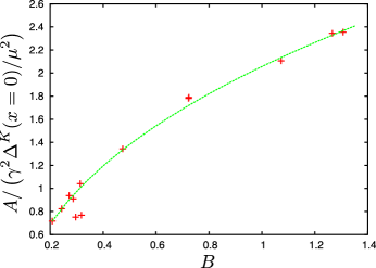
Figure 15: $A/(\gamma^{2}\Delta^{K}({\mathbf{x}}\!=\!0)/\mu^{2})$ versus $B$ for geometrically random lattices, where $A$ and $B$ are the fit parameters to the functional form ${\mathcal{G}(\mathbf{x})}=A\ln\left({\left|{\mathbf{x}}\right|}/B\right)$. The line is a fit to these data points using Eq. (92), assuming that there are long range correlations in the elastic moduli. [Color online]

We fit the measurements of ${\mathcal{G}(\mathbf{x})}$ to the functional form $A\ln\left({\left|{\mathbf{x}}\right|}/B\right)$ at large ${\left|{\mathbf{x}}\right|}$. This data is shown in Figure 15. For the very random lattices generated at low Lennard-Jones pressure ($T=8.0$, $P<0.3$) the values of $A/(\gamma^{2}\Delta^{K}({\mathbf{x}}\!=\!0)/\mu^{2})$ and $B$ are nearly constant, as our framework predicts for the simple case of delta-function spatial correlations. However, lattices created at higher pressure values ($T=8.0$, $P\geq 0.3$) showed significant growth of both $A/(\gamma^{2}\Delta^{K}({\mathbf{x}}\!=\!0)/\mu^{2})$ and $B$ with increasing pressure, reaching a saturation point at around $P=8.0$. Visual inspection of the lattices in question revealed subdomains of hexagonal crystalline ordering. Long range correlations in the connectivity implies long-range correlations in the elastic moduli, so we must apply the framework developed in Sec. III.5 and App. C.1 in order to fit the data for partially crystalline lattices. Once again, we try the functional form in Eq. (84) for the spatial correlations in the elastic modulus. The numerical value of the factor $g_{0}(\phi)$ can be calculated from the measured modulus autocorrelation $\Delta^{K}({\mathbf{x}}\!=\!0)$ using Eq. (89).

The fitting line in Fig. 15 represents a best fit of both the correlation exponent $\phi$ and the cutoff length $\Lambda^{-1}$ to the form

$$A \sim\frac{\Delta^{K}({\mathbf{x}}\!=\!0)\gamma^{2}}{\mu^{2}}\ \xi^{2}\left(1-\left(1+\left(\Lambda\xi\right)^{2}\right)^{1-\frac{\phi}{2}}\right)^{-1}$$

$$B \sim\frac{\xi}{\beta(\xi\Lambda,\phi)},$$ (92)

as suggested by Eq. (111). The best fit was achieved for $\phi=0.4$ and a cutoff length of $\Lambda^{-1}\approx 1.25$ lattice spacings. The corresponding analytic form of ${\mathcal{G}(\mathbf{x})}$ calculated from Eq. (80) using $g(u)$ from Eq. (84) is shown by the solid line in Fig. 14.

To test the predicted [Eq. (III.6)] $\cos 4\psi$ anisotropy in vorticity correlations, we measured $G_{\omega}({\mathbf{x}})$ as a function of the angle ${\mathbf{x}}$ makes with the $x$-axis. Figure 16 shows a polar plot of $G_{\omega}({\mathbf{x}})$, which clearly shows $\cos 4\psi$ behavior, and the dependence of the $\cos 4\psi$ term on $|{\mathbf{x}}|$, which shows the expected $|{\mathbf{x}}|^{-2}$ behavior.

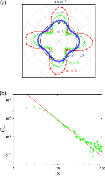
Figure 16: (a) Polar plot showing the $\cos 4\psi$ modulation of the vorticity correlation function $G_{\omega}({\mathbf{x}})$ for ${\left|{\mathbf{x}}\right|}=2$, $5$, and $10$ lattice spacings. (b) A log-log plot of the coefficient of $\cos 4\psi$ in $G_{\omega}({\mathbf{x}})$ showing the expected $|{\mathbf{x}}|^{-2}$ fall off at large $|{\mathbf{x}}|$. [Color online]

IV.4 Model D: Random lattice with internal stresses

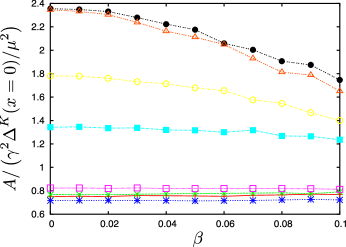
Figure 17: $A/(\gamma^{2}\Delta^{K}({\mathbf{x}}\!=\!0)/\mu^{2})$ versus $\beta$ for geometrically random lattices with internal stresses, where $A$ is the coefficient of a logrithmic fit to the non-affinity correlation function ${\mathcal{G}(\mathbf{x})}$ for each lattice and $\beta$ is the bond frustration factor used to induce internal stresses. The lines are for lattices with eight different temperature-pressure combinations, with $T=8.0$ and, from bottom to top $P=0.025$, $0.05$, $0.1$, $0.2$, $0.4$, $0.6$, $0.8$, and $1.0$, all in units of the Lennard-Jones potential. [Color online]

Finally, we simulate the most general model for random lattices, in which the rest bond length $R_{bR}$ is not equal to the equilibrium lattice parameter $R_{b0}$, and the lattice parameters $R_{b0}$ along with the number of bonds per node are random to within some finite distribution. Each bond is assigned the anharmonic potential of Eq. (88), where the spring constant $k_{b}(R_{b})=k_{0}/R_{b}$ is a constant per unit length of the rest bond length. We used the same geometrically random lattices from Section IV.3 as staring points, then we add bond length frustration using the technique from Section IV.2: We multiply the rest lengths of all bonds by a factor $(1+\beta_{b})$ where $\beta_{b}$ is chosen randomly from a flat distribution lying between $-\beta$ and $\beta$ with $\beta<0.1$. We find the equilibrium configuration of the lattice by minimizing the elastic energy over node positions and box size. We then shear the lattice by $0.1\%$, minimize the energy over node positions, and measure the non-affinity correlation function ${\mathcal{G}(\mathbf{x})}$.

In all these simulations, the correlation function ${\mathcal{G}(\mathbf{x})}$ was well fit by the functional form $A\ln\left({\left|{\mathbf{x}}\right|}/B\right)$. Figure 17 shows a plot of $A/(\gamma^{2}\Delta^{K}({\mathbf{x}}\!=\!0)/\mu^{2})$ for all data sets as a function of $\beta$. The data points for $\beta=0$ correspond to the data from Section IV.3; their deviation from the expected constancy of $A/(\gamma^{2}\Delta^{K}({\mathbf{x}}\!=\!0)/\mu^{2})$ was explained in that section by the growth of a correlation length scale as the system acquires partial hexagonal crystalline ordering. Here we see that as $\beta$ is increased, the long length scale ordering is disrupted by the additional randomness, and the ratio $A/(\gamma^{2}\Delta^{K}({\mathbf{x}}\!=\!0)/\mu^{2})$ decreases toward the value for completely disordered lattices.

V Summary and Conclusions

Nonaffine distortions are always present in random elastic networks subjected to external stress. In this paper, using both analytical and numerical techniques, we study properties of nonaffinity in these systems manifested in correlation functions of the deviation, ${\mathbf{u}}^{\prime}({\mathbf{x}})$, of local displacements from their affine form. We introduce four models of random elastic networks with random local elastic moduli and possibly local random stress arising either from randomness in the form of the central force potentials between nearest neighbor sites or from random connectivity of the the network. In all cases, we show analytically and verify with numerical simulations that random elastic modulus times imposed strain and not random stress act as sources for nonaffine distortions. We calculate the nonaffinity displacement correlation function, ${\mathcal{G}(\mathbf{x})}=\langle[{\mathbf{u}}^{\prime}({\mathbf{x}})-{\mathbf{u}}^{\prime}(0)]^{2}\rangle$, and the vorticity correlation function, $G_{\omega}({\mathbf{x}})=\langle\omega({\mathbf{x}})\omega(0)\rangle$ analytically and verify their form in numerical simulations for systems with both short- and long-range correlations in local elastic moduli. We show in particular that ${\mathcal{G}(\mathbf{x})}\sim\gamma^{2}(\langle(\delta K)^{2}\rangle/K^{2})\ln|{\mathbf{x}}|$ at large ${\mathbf{x}}$ in two dimensions, where $\gamma$ is the imposed strain, $K$ is the average of elastic modulus, and $\langle(\delta K)^{2}\rangle$ is it variance.

The formalism we develop is general and should be applicable to any elastic system that has a well defined average shear modulus. It should provide a basis for studying nonaffinity in granular media, foams, networks of semi-flexible polymers, and related systems. It should, in particular, provide a method of calculating correlation lengths near percolation-like thresholds such as the $J$-point in jammed systems or the rigidity percolation point. We have begun Vernon et al. (2005) to use these techniques to calculate correlation lengths in the former systems which we will eventually compared with those calculated from the density of states Wyart et al. (2005); Silbert et al. (2005) and to study nonaffinity in networks of semi-flexible polymers Didonna and Levine (2005).

Appendix A Properties of the modulus correlator

The modulus correlator $\Delta^{K}_{ijkl;i^{\prime}j^{\prime}k^{\prime}l^{\prime}}({\mathbf{q}})$ is an 8th rank tensor. The number of its independent components depends on the symmetry of the reference space. In this appendix, we will determine the number and form of its independent components at ${\mathbf{q}}=0$ (strictly speaking ${\mathbf{q}}\rightarrow 0$), or, equivalently, at all ${\mathbf{q}}$ when correlations are short range and it is independent of ${\mathbf{q}}$, when the reference space is isotropic. In this case, the general form of $\Delta^{K}_{ijkl;i^{\prime}j^{\prime}kj^{\prime}l^{\prime}}\equiv\Delta^{K}_{ijkl;i^{\prime}j^{\prime}k^{\prime}l^{\prime}}({\mathbf{q}}=0)$ must be constructed from products of Kroneker $\delta$’s that distinctly pair all indices while respecting all symmetries.

It is useful to recall how this process is carried out for the simpler case of the 4th-rank elastic-modulus tensor $K_{ijkl}$, which is symmetric under interchange of $i$ and $j$, of $k$ and $l$, and of the pairs $ij$ and $kl$. Since any index can be paired with any of the remaining three and there is only one way to pair the remaining two, there are three distinct Kroneker-$\delta$ pairings, which we will call contractions, of the four indices: $\delta_{ij}\delta_{kl}$, $\delta_{ik}\delta_{jl}$, and $\delta_{il}\delta_{jk}$. The first of these satisfies all of the symmetry constraints, but the second two do not; their sum, however, does. The elastic-modulus tensor, therefore, has two independent components in an isotropic medium: $K_{ijkl}=\lambda\delta_{ij}\delta_{kl}+\mu(\delta_{ik}\delta_{jl}+\delta_{il}\delta_{jk})$.

$\Delta^{K}_{ijkl;i^{\prime}j^{\prime}k^{\prime}l^{\prime}}$ is symmetric under interchange of $i$ and $j$, $k$ and $l$, $i^{\prime}$ and $j^{\prime}$, and $k^{\prime}$ and $l^{\prime}$; under the interchange of the pairs $ij$ and $kl$ and of the pairs $i^{\prime}j^{\prime}$ and $k^{\prime}l^{\prime}$; and under the interchange of the four-plets $ijkl$ and $i^{\prime}j^{\prime}k^{\prime}l^{\prime}$. The total number of possible contractions of these 8 indices is $N_{T}=7\times 5\times 3\times 1=105$ because any index can be contracted with any of the seven remaining indices, any one of the six remaining indices can then be contracted with any of the other five remaining, etc. Most of the individual realizations of these 105 possible contractions will not satisfy symmetry constraints; it is necessary to find the linear combinations of them that do. Figure 18 provides a graphical representation of the eight distinct contraction groups the sum over whose elements satisfy all constraints. The elastic-modulus correlation function in an isotropic medium can thus be written as

$$\Delta^{K}_{ijkl;i^{\prime}j^{\prime}k^{\prime}l^{\prime}}=\sum_{\alpha}\Delta_{ijkl;i^{\prime}j^{\prime}k^{\prime}l^{\prime}}^{K\alpha}$$

$$=\Delta_{1}\delta_{ij}\delta_{kl}\delta_{i^{\prime}j^{\prime}}\delta_{k^{\prime}l^{\prime}}$$

$$+\Delta_{2}\delta_{ij}\delta_{kl}(\delta_{i^{\prime}k^{\prime}}\delta_{j^{\prime}l^{\prime}}+\delta_{i^{\prime}l^{\prime}}\delta_{j^{\prime}k^{\prime}})+\text{prime}\leftrightarrow\text{unprime}$$

$$+\Delta_{3}(\delta_{ik}\delta_{jl}+\delta_{il}\delta_{jk})(\delta_{i^{\prime}k^{\prime}}\delta_{j^{\prime}l^{\prime}}+\delta_{i^{\prime}l^{\prime}}\delta_{j^{\prime}l^{\prime}})$$

$$+\Delta_{4}\delta_{ij}\delta_{i^{\prime}j^{\prime}}\delta_{kk^{\prime}}\delta_{ll^{\prime}}+\text{7 perm.}$$

$$+\Delta_{5}\delta_{ij}\delta_{i^{\prime}k^{\prime}}\delta_{kj^{\prime}}\delta_{ll^{\prime}}+\text{31 perm.}$$

$$+\Delta_{6}\delta_{ik}\delta_{i^{\prime}k^{\prime}}\delta_{jj^{\prime}}\delta_{ll^{\prime}}+\text{31 perm.}$$

$$+\Delta_{7}\delta_{ii^{\prime}}\delta_{jj^{\prime}}\delta_{kk^{\prime}}\delta_{ll^{\prime}}+\text{7 perm.}$$

$$+\Delta_{8}\delta_{ii^{\prime}}\delta_{jk^{\prime}}\delta_{kj^{\prime}}\delta_{ll^{\prime}}+\text{15 perm.}$$ (93)

where $\Delta^{K1}_{ijkl;i^{\prime}j^{\prime}k^{\prime}l^{\prime}}=\Delta_{1}\delta_{ij}\delta_{kl}\delta_{i^{\prime}j^{\prime}}\delta_{k^{\prime}l^{\prime}}$, etc. The first three terms in $\Delta^{K}_{ijkl;i^{\prime}j^{\prime}k^{\prime}l^{\prime}}$ describe correlations in the isotropic Lamé coefficients: $\Delta_{1}=\langle(\delta\lambda)^{2}\rangle$, $\Delta_{2}=\langle\delta\lambda\delta\mu\rangle$, and $\Delta_{3}=\langle(\delta\mu)^{2}\rangle$. The other terms represent fluctuations away from local isotropy.

Figure 18: This figure provides a graphical representation of the groups of contractions that are invariant under the symmetry operations that leave $\Delta^{K}_{ijkl;i^{\prime}j^{\prime}k^{\prime}l^{\prime}}$ unchanged. It shows 8 graphs representing contractions, none of which are transformed into any of the others under any symmetry operation. The symmetry operations applied to each contraction will, however, generate other contractions. The number of contractions for each graph produced by performing all symmetry operations on it is indicated below each graph along with a representation of the graph in terms of Kronecker $\delta$’s.

Appendix B Evaluation of $G({\mathbf{q}})$

We outline here the calculation of $G({\mathbf{q}})$ to lowest order in $\Delta^{K}$ in isotropic systems. We use Eq. (49) for $G_{ij}({\mathbf{q}})$ and sum over $i=j$. Using Eq. (51), we find

$$\ \chi_{ip}^{0}({\mathbf{q}})\chi_{ip^{\prime}}^{0}({\mathbf{q}})=\frac{1}{\mu^{2}q^{4}}\delta_{pp^{\prime}}^{T}+\frac{1}{(\lambda+2\mu)^{2}q^{4}}{\hat{q}}_{p}{\hat{q}}_{p^{\prime}},$$ (94)

where ${\hat{q}}_{p}=q_{p}/q$ and $\delta_{pp^{\prime}}^{T}=\delta_{pp^{\prime}}-{\hat{q}}_{p}{\hat{q}}_{p^{\prime}}$. Then

$$G({\mathbf{q}})=\gamma_{xy}^{2}\sum_{\alpha=1}^{8}\left(\frac{1}{\mu^{2}q^{2}}S_{\alpha}^{T}+\frac{1}{(\lambda+2\mu)^{2}q^{2}}S_{\alpha}^{L}\right),$$ (95)

where

$$S_{\alpha}^{T}=\delta_{pp^{\prime}}^{T}S_{\alpha pp^{\prime}}\qquad S_{\alpha}^{L}={\hat{q}}_{p}{\hat{q}}_{p^{\prime}}S_{\alpha pp^{\prime}},$$ (96)

with

$$S_{\alpha pp^{\prime}}=\Delta^{K\alpha}_{pjxy;p^{\prime}j^{\prime}xy}{\hat{q}}_{j}{\hat{q}}_{j^{\prime}}$$ (97)

where $\Delta^{K\alpha}_{ijkl;i^{\prime}j^{\prime}k^{\prime}l^{\prime}}$ is defined in Eq. (93). It is straightforward but tedious to calculate $S_{\alpha}^{T}$ and $S_{\alpha}^{L}$ from Eq. (93). The results are

$$\begin{array}[]{ll}S_{1}^{T}=S_{2}^{T}=0,&S_{1}^{L}=S_{2}^{L}=0;\\ S_{3}^{T}=\Delta_{3}^{T}({\hat{q}}_{\perp}^{2}-4{\hat{q}}_{x}^{2}{\hat{q}}_{y}^{2}),&S_{3}^{L}=\Delta_{3}^{L}{\hat{q}}_{x}^{2}{\hat{q}}_{y}^{2};\\ S_{5}^{T}=0,&S_{5}^{L}=\Delta_{5}^{L}4{\hat{q}}_{\perp}^{2}\\ S_{6}^{T}=\Delta_{6}^{T}(2+d{\hat{q}}_{\perp}^{2}-16{\hat{q}}_{x}^{2}),&S_{6}^{L}=\Delta_{6}^{L}(4{\hat{q}}_{\perp}^{2}+16{\hat{q}}_{x}^{2}{\hat{q}}_{y}^{2});\\ S_{7}^{T}=\Delta_{7}^{T}[(d-1)+{\hat{q}}_{\perp}^{2}-4{\hat{q}}_{x}^{2}{\hat{q}}_{y}^{2}];&S_{7}^{L}=\Delta_{7}^{L}(2+4{\hat{q}}_{x}^{2}{\hat{q}}_{y}^{2})\\ S_{8}^{T}=\Delta_{8}^{T}[2+(d-2){\hat{q}}_{\perp}^{2}],&S_{8}^{L}=\Delta_{8}^{L}4{\hat{q}}_{\perp}^{2}.\end{array}$$ (98)

Appendix C Evaluation of ${\mathcal{G}({\mathbf{x}})}$

In this appendix, we will evaluate the integrals [Eq. (79)]

$$\mathcal{F}_{\alpha}=2\xi^{\phi}\int\frac{d^{d}q}{(2\pi)^{d}}\frac{1}{q^{2}}f_{\alpha}({\mathbf{q}})g_{\alpha}(q\xi)\left(1-e^{i{\mathbf{q}}\cdot{\mathbf{x}}}\right)$$ (99)

in $2D$ and $3D$ that make up the function ${\mathcal{G}(\mathbf{x})}$, where $f_{A}({\mathbf{q}})=1$, $f_{B}({\mathbf{q}})=\hat{q}_{\perp}^{2}$, and $f_{C}({\mathbf{q}})=\hat{q}_{x}^{2}\hat{q}_{y}^{2}$.

C.1 Two dimensions

In two dimensions, $f_{B}({\mathbf{q}})=1=f_{A}({\mathbf{q}})$, and

$$f_{C}({\mathbf{q}})=\sin^{2}\phi_{q}\cos^{2}\phi_{q}=\frac{1}{8}(1-\cos 4\phi_{q}),$$ (100)

where $\phi_{q}$ is the angle between ${\mathbf{q}}$ and the $x$-axis. Using the plane-wave decomposition relation

$$e^{i{\mathbf{q}}\cdot{\mathbf{x}}}=J_{0}(q|{\mathbf{x}}|)+2\sum_{n=1}^{\infty}\cos n\Theta J_{n}(q|{\mathbf{x}}|),$$ (101)

where $J_{n}(x)$ is the $n$th order Bessel function, $\Theta=\phi_{q}-\psi$, and $\psi$ is the angle between ${\mathbf{x}}$ and the $x$-axis, and the orthogonality relation

$$\frac{1}{2\pi}\int_{0}^{2\pi}d\phi\cos n\psi\cos m\Theta=\begin{cases}\frac{1}{2}\delta_{nm}\cos n\psi&n\neq 0\\ \delta_{nm}&n=0\end{cases},$$ (102)

we find

$$\mathcal{F}_{\alpha}\equiv F_{I}[g_{\alpha}]=\frac{\xi^{\phi}}{\pi}\int_{0}^{\Lambda}\frac{dq}{q}g_{\alpha}(q\xi)[1-J_{0}(q|{\mathbf{x}}|)]$$ (103)

for $\alpha=A,B$ and

$$\mathcal{F}_{C}=\mathcal{F}_{I}[g_{C}]-\cos 4\psi F_{A}[g_{C}],$$ (104)

where

$$F_{A}[g_{\alpha}]=\frac{\xi}{\pi}\int_{0}^{\Lambda}\frac{dq}{q}g_{\alpha}(q\xi)J_{4}(q|{\mathbf{x}}|).$$ (105)

Thus,

$$\mathcal{F}({\mathbf{x}})=F_{I}[g]+\frac{1}{8}\cos 4\psi F_{A}[g_{C}],$$ (106)

where

$$g(q\xi)=g_{A}(q\xi)+g_{B}(q\xi)-\frac{1}{8}g_{C}(q\xi).$$ (107)

We now evaluate the integrals $F_{I}$ and $F_{A}$ in the limits $|{\mathbf{x}}|\gg\xi\geq\Lambda^{-1}$ and $\Lambda^{-1}\ll|{\mathbf{x}}|\ll\xi$.

C.1.1 $|{\mathbf{x}}|\gg\xi\geq\Lambda^{-1}$ in Two Dimensions

To evaluate the first limit of $F_{I}$, we set $y=q|{\mathbf{x}}|$ in Eq. (103):

$$F_{I}[g]=\frac{\xi^{\phi}}{\pi}\Big{\{}\int_{1}^{\Lambda|{\mathbf{x}}|}\frac{dy}{y}g(y\xi/|{\mathbf{x}}|)$$

$$+\int_{0}^{1}\frac{dy}{y}g(y\xi/|{\mathbf{x}}|)[1-J_{0}(y)]-\int_{1}^{\Lambda|{\mathbf{x}}|}\frac{dy}{y}g(y\xi/|{\mathbf{x}}|)J_{0}(y)\Big{\}}.$$ (108)

In the limit $|{\mathbf{x}}|/\xi\rightarrow\infty$, we can safely replace $g(y\xi/|{\mathbf{x}}|)$ by $g_{0}$ in the second and third integrals in this expression, and we can let $\Lambda|{\mathbf{x}}|\rightarrow\infty$ in the third integral. The first integral diverges as $\ln|{\mathbf{x}}|$ if we replace $g(y\xi/|{\mathbf{x}}|)$ by $g_{0}$ in it, and we have to be more careful to extract the constant term beyond the log:

$$\int_{1}^{\Lambda|{\mathbf{x}}|} \frac{dy}{y}g(y\xi/|{\mathbf{x}}|)=\int_{\xi/|{\mathbf{x}}|}^{1}\frac{du}{u}g(u)+\int_{1}^{\Lambda\xi}\frac{du}{u}g(u)$$ (109)

$$\rightarrow g_{0}\ln|{\mathbf{x}}|/\xi+\int_{0}^{1}\frac{du}{u}[g(u)-g_{0}]+\int_{1}^{\Lambda\xi}\frac{du}{u}g(u).$$ (110)

Thus in the limit $|{\mathbf{x}}|\gg\xi\geq\Lambda^{-1}$,

$$F_{I}[g]=\frac{\xi^{\phi}}{\pi}g_{0}\ln\beta(\Lambda\xi,\phi)\frac{|{\mathbf{x}}|}{\xi},$$ (111)

where

$$\ln\beta(\Lambda\xi,\phi)=\ln\alpha+\int_{0}^{1}\frac{dy}{y}\left[\frac{g(y)}{g_{0}}-1\right]+\int_{1}^{\Lambda\xi}\frac{dy}{y}\frac{g(y)}{g_{0}},$$ (112)

where

$$\ln\alpha=\int_{0}^{1}\frac{dy}{y}[1-J_{0}(y)]-\int_{1}^{\infty}\frac{dy}{y}J_{0}(y)=-0.1159$$ (113)

and $\alpha=0.8905$. When $g(y)=g_{0}$, independent of $y$,

$$\ln\beta(\Lambda\xi)\rightarrow\ln\alpha+\ln\Lambda\xi,$$ (114)

and Eq. (108) reduces to Eq. (44b) when $g_{0}\xi^{\phi}$ is identified with $\Delta^{S}$.

The $|{\mathbf{x}}|\gg\xi$ limit of $F_{A}$ is obtained by setting $y=q|{\mathbf{x}}|$ and noting that letting the upper limit of the integral go to infinity and replacing $g(y|{\mathbf{x}}|/\xi)$ by $g_{0}$ introduces no singularities. The result is

$$F_{A}[g]=\frac{\xi}{\pi}g_{0}\int_{0}^{\infty}\frac{dy}{y}J_{4}(y)=\frac{g_{0}\xi}{4}.$$ (115)

C.1.2 $\Lambda^{-1}\ll|{\mathbf{x}}|\ll\xi$ in Two Dimensions

To evaluate integrals when $\Lambda^{-1}\ll|{\mathbf{x}}|\ll\xi$, we introduce a new function

$$h(u)=u^{\phi}\frac{g(u)}{g_{\infty}}\sim\begin{cases}1&\text{as $u\rightarrow\infty$},\\ (g_{0}/g_{\infty})u^{\phi}&\text{as $u\rightarrow 0$},\end{cases}$$ (116)

where $g_{\infty}$ is defined in Eq. (78) Then $\mathcal{F}_{I}[g]=g_{\infty}(\xi^{\phi}/\pi)(|{\mathbf{x}}|/\xi)^{\phi}\mathcal{I}({\mathbf{x}})$, where

$$\mathcal{I}=\int_{0}^{\Lambda|{\mathbf{x}}|}\frac{dy}{y}y^{-\phi}h(y\xi/|{\mathbf{x}}|)[1-J_{0}(y)].$$ (117)

This integral has a potential infrared divergence as $\xi/|{\mathbf{x}}|\rightarrow\infty$ when $\phi\geq 2$. To isolate it, we break up the integral from $0$ to $\Lambda|{\mathbf{x}}|$ into one from $0$ to $1$ and another from $1$ to $\Lambda|{\mathbf{x}}|$. There are no troubles with ultraviolet divergences in the second integral, and in it, we can let $\Lambda|{\mathbf{x}}|\rightarrow\infty$ and replace $h(y\xi/|{\mathbf{x}}|)$ by its infinite argument limit of one. In the integral from $0$ to $1$, we extract the small $y$ behavior of $1-J_{0}(y)$ via $1-J_{0}(y)=(y^{2}/4)+[1-J_{0}(y)-(y^{2}/4)]$. The second part of this expression vanishes as $y^{4}$ at small $y$, and there is no infrared divergence in the integral involving it so long as $\phi<4$. Thus, we have

$$\mathcal{I}=\mathcal{I}_{1} +\int_{0}^{1}\frac{dy}{y}y^{-\phi}[1-J_{0}(y)-(y^{2}/4)]$$ (118)

$$+\int_{1}^{\infty}\frac{dy}{y}y^{-\phi}[1-J_{0}(y)],$$ (119)

where

$$\mathcal{I}_{1} =\frac{1}{4}\int_{0}^{1}dyy^{1-\phi}h(y\xi/|{\mathbf{x}}|),$$ (120)

$$=\frac{1}{4}\left(\frac{\xi}{|{\mathbf{x}}|}\right)^{\phi-2}\int_{0}^{\xi/|{\mathbf{x}}|}duu^{1-\phi}h(u)$$ (121)

$$=\frac{1}{4}\left(\frac{\xi}{|{\mathbf{x}}|}\right)^{\phi-2}\Big{\{}\int_{0}^{1}duu^{1-\phi}h(u)$$ (122)

$$\qquad+\int_{1}^{\xi/|{\mathbf{x}}|}dyu^{1-\phi}+\int_{1}^{\xi/|{\mathbf{x}}|}u^{1-\phi}[h(u)-1]\Big{\}}.$$ (123)

Using $\int_{1}^{\eta}u^{1-\phi}=[\eta^{2-\phi}-1]/(2-\phi)$, we arrive at Eq. (82) with

$$\mathcal{A}_{2}(\phi) =\int_{0}^{\infty}dyy^{-(1+\phi)}[1-J_{0}(y)]$$ (124)

$$\ln\nu =\int_{0}^{1}\frac{du}{u}h(u)+\int_{1}^{\infty}\frac{du}{u}[h(u)-1]$$ (125)

$$\mathcal{C}_{2}(\phi) =\int_{0}^{\infty}duu^{1-\phi}h(u).$$ (126)

The evaluation of the $\xi\gg|{\mathbf{x}}|$ limit of $F_{A}[g]$ is straightforward. The result is

$$F_{A}=g_{\infty}\frac{|{\mathbf{x}}|^{\phi}}{\pi}\int_{0}^{\infty}\frac{dy}{y}y^{-\phi}J_{4}(y).$$ (127)

C.2 Three Dimensions

To evaluate the integrals $\mathcal{F}_{\alpha}$ in $3D$, we make use of the $3D$ plane-wave decomposition:

$$e^{i{\mathbf{q}}\cdot{\mathbf{x}}}=4\pi\sum_{l=0}^{\infty}i^{l}j_{l}(q|{\mathbf{x}}|)\sum_{m=-l}^{l}Y_{lm}(\Omega_{q})Y_{lm}^{*}(\Omega_{x}),$$ (128)

where $\Omega_{q}=(\theta_{q},\phi_{q})$ and $\Omega_{x}=(\theta_{x},\phi_{x})$ are, respectively, the polar angles of ${\mathbf{q}}$ and ${\mathbf{x}}$, $Y_{lm}(\Omega)$ are spherical harmonics, and $j_{n}(u)$ is the $n$th order spherical Bessel function. Then, noting that

$${\hat{q}}_{\perp}^{2} =\sin^{2}\theta_{q}=\frac{2}{3}\left[1-P_{2}(\cos\theta_{q})\right],$$ (129)

$${\hat{q}}_{x}^{2}{\hat{q}}_{y}^{2} =\frac{1}{8}\sin^{2}\theta_{q}(1-\cos 4\phi_{q})$$ (130)

$$=\frac{1}{105}[7-10P_{2}(\cos\theta_{q})+3P_{4}(\cos\theta_{q})]$$ (131)

$$\,\,\,-\frac{1}{16}\sqrt{\frac{4\pi}{9!}}2^{4}4![Y_{44}(\Omega_{q})+Y_{4,-4}(\Omega_{q})],$$ (132)

where $P_{n}(x)$ is the $n$th-order Legendre Polynomial, we find

$$\mathcal{F}_{A} =\frac{\xi^{\phi}}{\pi}I_{0}[g_{A}]$$ (133)

$$\mathcal{F}_{B} =\frac{\xi^{\phi}}{\pi}\left\{\frac{2}{3}I_{2}[g_{B}]+\frac{2}{3}P_{2}(\cos\theta_{x})I_{2}[g_{B}]\right\}$$ (134)

$$\mathcal{F}_{C} =\frac{\xi^{\phi}}{\pi}\Big{\{}\frac{1}{15}I_{0}[g_{C}]-\frac{2}{21}P_{2}(\cos\theta_{x})I_{2}[g_{C}]$$ (135)

$$\,\,\,-\left[\frac{1}{35}P_{2}(\cos\theta_{x})+\frac{1}{8}\sin^{2}\theta_{x}\cos 4\phi_{x}\right]I_{4}[g_{C}],$$ (136)

where

$$I_{0}[g] =\int_{0}^{\Lambda}dqg(q\xi)[1-j_{0}(q|{\mathbf{x}}|)]$$ (137)

$$I_{2}[g] =\int_{0}^{\Lambda}dqg(q\xi)j_{2}(q|{\mathbf{x}}|)$$ (138)

$$I_{4}[g] =\int_{0}^{\Lambda}dqg(q\xi)j_{4}(q|{\mathbf{x}}|).$$ (139)

Thus,

$$\mathcal{F} =\mathcal{F}_{A}+\mathcal{F}_{B}-\mathcal{F}_{C}$$ (140)

$$=\frac{\xi^{\phi}}{\pi}\Big{\{}I_{1}[g_{1}]+P_{2}(\cos\theta_{x})I_{2}[g_{2}]$$ (141)

$$\qquad\left[\frac{1}{35}P_{2}(\cos\theta_{x})+\frac{1}{8}\sin^{2}\theta_{x}\cos 4\phi_{x}\right]I_{4}[g_{C}],$$ (142)

where $g_{1}=g_{A}+\frac{2}{3}g_{B}-\frac{1}{15}g_{C}$ and $g_{2}=\frac{2}{3}g_{B}+\frac{2}{21}g_{C}$. Thus we need only evaluate the three integrals $I_{1}$, $I_{2}$, and $I_{3}$.

C.2.1 $|{\mathbf{x}}|\gg\xi>\Lambda^{-1}$ in Three Dimensions

In this limit, in integrals with integrands proportional to $j_{n}(q|{\mathbf{x}}|)$, we set $y=q|{\mathbf{x}}|$, replace $g(y\xi/|{\mathbf{x}}|)$ by $g_{0}$ and replace the upper limit, $\Lambda|{\mathbf{x}}|$, of integration by $\infty$. In the part of the integral $I_{1}$ not proportional to $j_{0}(q|{\mathbf{x}}|)$, we set $y=q\xi$. The result is

$$I_{1} \sim g_{0}\frac{\pi}{2}\left[\frac{2}{\pi}\int_{0}^{\Lambda\xi}\frac{g(y)}{g_{0}}dy-\frac{1}{|{\mathbf{x}}|}\right]$$ (143)

$$I_{2} \sim\frac{g_{0}}{|{\mathbf{x}}|}\int_{0}^{\infty}dyj_{2}(y)=\frac{g_{0}\pi}{4|{\mathbf{x}}|}$$ (144)

$$I_{3} \sim\frac{g_{0}}{|{\mathbf{x}}|}\int_{0}^{\infty}j_{4}(y)=\frac{3g_{0}\pi}{16|{\mathbf{x}}|}.$$ (145)

C.2.2 $\Lambda^{-1}\ll|{\mathbf{x}}|\ll\xi$ in Three Dimensions

To treat this limit, as in $2D$, we use the function $h(u)$ [Eq. ( 116)]. To evaluate $I_{1}$, we break up the limits of integration in much the same way we did in $2D$. The result is

$$I_{1} =g_{\infty}\xi^{-\phi}|{\mathbf{x}}|^{\phi-1}$$ (146)

$$\,\,\times\Big{\{}\int_{0}^{1}dyy^{-\phi}[1-j_{0}(y)]-\int_{1}^{\infty}dyy^{-\phi}j_{0}(y)$$ (147)

$$\qquad+\frac{1}{1-\phi}[(\Lambda|{\mathbf{x}}|)^{1-\phi}-1]$$ (148)

$$\qquad+\left(\frac{\xi}{|{\mathbf{x}}|}\right)^{1-\phi}\int_{0}^{\Lambda\xi}duu^{-\phi}[h(u)-1]\Big{\}}$$ (149)

for $0<\phi<3$. The dominant behavior for $1<\phi<3$ and $0<\phi<1$ is then

$$I_{1}\sim\begin{cases}g_{\infty}\xi^{-\phi}|{\mathbf{x}}|^{\phi-1}\mathcal{A}_{3}(\phi)&\text{$1<\phi<3$}\\ \frac{1}{\xi}\int_{0}^{\Lambda\xi}dug(u)-g_{\infty}\xi^{-\phi}|{\mathbf{x}}|^{-(1-\phi)}\mathcal{C}_{3}(\phi)&\text{$0<\phi<1$}.\end{cases},$$ (150)

where

$$\mathcal{A}_{3}(\phi) =\int_{0}^{\infty}y^{-\phi}[1-j_{0}(y)]$$ (151a)

$$\mathcal{C}_{3}(\phi) =\int_{0}^{\infty}y^{-\phi}j_{0}(y).$$ (151b)

C.3 One Dimension

In $1D$, there is only one function to evaluate

$${\mathcal{F}}(x) =2\xi^{\phi}\int_{-\Lambda}^{\Lambda}\frac{dq}{2\pi}\frac{1}{q^{2}}g(q\xi)[1-\cos(q|x|)]$$

$$=\frac{2\xi^{\phi}}{\pi}\int_{0}^{\Lambda|x|}dy\frac{1}{y^{2}}g(y\xi/|x|)(1-\cos y).$$ (152)

The limit $|x|\gg\xi$ is obtained as before by replacing $g(y\xi/|x|)$ with $g_{0}$ and letting $\Lambda|x|\rightarrow\infty$:

$${\mathcal{F}}(x)=\frac{2}{\pi}|x|g_{0}\xi^{\phi}\int_{0}^{\infty}dy\frac{1-\cos y}{y^{2}}=g_{0}\xi^{\phi}|x|.$$ (153)

In the limit $\Lambda^{-1}\ll|x|\ll\xi$, we introduce $h(y)$ as in $2D$ and $3D$: ${\mathcal{F}}(x)=(2g_{\infty}|x|/\pi){\mathcal{K}}$, where

$${\mathcal{K}} = \int_{0}^{\Lambda|x|}dyh(y\xi/|x|)y^{-(2+\phi)}(1-\cos y)$$

$$= {\mathcal{K}}_{1}+\int_{0}^{1}dyy^{-(2+\phi)}[1-\cos y-(y^{2}/2)]$$

$$+\int_{1}^{\infty}y^{-(2+\phi)}[1-\cos y],$$ (154)

where

$${\mathcal{K}}_{1} = \frac{1}{2}\int_{0}^{1}dyy^{-\phi}h(y\xi/|x|)$$

$$= \frac{1}{2}\left(\frac{\xi}{|x|}\right)^{\phi-1}\Big{\{}\frac{1}{1-\phi}\Big{(}\left(\frac{\xi}{|x|}\right)^{1-\phi}-1\Big{]}$$

$$+\int_{0}^{2}duh(u)u^{-\phi}+\int_{1}^{\infty}duu^{-\phi}[h(u)-1]\Big{\}}.$$

Combining Eqs. (154) with (C.3), we find

$${\mathcal{F}}(x)\sim\begin{cases}\frac{2}{\pi}g_{\infty}|x|^{1+\phi}\mathcal{A}_{1}(\phi)&\text{if $\phi<1$},\\ \frac{1}{\pi}\ln\nu\xi/|x|&\text{if $\phi=1$},\\ \frac{1}{\pi}\xi^{\phi-1}|x|^{2}\mathcal{C}_{2}(\phi)&\text{if $\phi>1$},\end{cases}$$ (156)

where $\nu$ is given by Eq. ( 125) and $\mathcal{C}_{2}(\phi)$ is given by Eq. (126) and where

$$\mathcal{A}_{1}=\int_{0}^{\infty}\frac{1-\cos y}{y^{2+\phi}}.$$ (157)

The $|{\mathbf{x}}|\ll\xi$ limits of both $I_{2}$ and $I_{3}$ can be obtained by simply by replacing $g(q\xi)$ by $(q\xi)^{-\phi}g_{\infty}$:

$$I_{2} \sim g_{\infty}\xi^{-\phi}|{\mathbf{x}}|^{\phi-1}\int_{0}^{\infty}dyy^{-\phi}j_{2}(y) 0<\phi<3$$ (158)

$$I_{3} \sim g_{\infty}\xi^{-\phi}|{\mathbf{x}}|^{\phi-1}\int_{0}^{\infty}dyy^{-\phi}j_{4}(y) \text{$0<\phi<5$}.$$ (159)

Appendix D Evaluation of $\cal{G}_{\omega}({\mathbf{x}})$

In this appendix we will evaluate the rotational correlation function $G_{\omega}({\mathbf{x}})$ in two dimensions. To lowest order in $\Delta^{K}$,

$$G_{\omega}({\mathbf{q}})=\frac{1}{4}\epsilon_{ri}\epsilon_{r^{\prime}i^{\prime}}q_{r}q_{r^{\prime}}\chi_{ip}^{0}({\mathbf{q}})\chi_{i^{\prime}p^{\prime}}^{0}(-{\mathbf{q}})\sum_{\alpha}S_{\alpha pp^{\prime}},$$ (160)

where $S_{\alpha pp^{\prime}}$ is defined in Eq. (97). The product $\epsilon_{ri}\epsilon_{r^{\prime}i^{\prime}}$ is simply $\delta_{rr^{\prime}}\delta_{ii^{\prime}}-\delta_{ri^{\prime}}\delta_{ir^{\prime}}$, and $\epsilon_{ri}\epsilon_{r^{\prime}i^{\prime}}q_{r}q_{r}^{\prime}=q^{2}\delta_{ii^{\prime}}^{T}$. When this operates on $\chi_{ip}^{0}\chi_{i^{\prime}p^{\prime}}^{0}$, it projects out the transverse part leaving $\delta_{pp^{\prime}}^{T}/(\mu^{2}q^{2})$. Thus

$$G_{\omega}({\mathbf{q}})=\frac{\gamma_{xy}^{2}}{\mu^{2}}\sum_{\alpha}S_{\alpha}^{T}=\frac{\gamma_{xy}^{2}}{\mu^{2}}(\Delta_{A}^{\omega}-\Delta_{C}^{\omega}{\hat{q}}_{x}^{2}{\hat{q}}_{y}^{2}).$$ (161)

where $\Delta_{A}^{\omega}=\Delta_{3}+4\Delta_{6}+2\Delta_{7}+2\Delta_{8}$ and $\Delta_{C}^{\omega}=4\Delta_{3}+15\Delta_{6}+4\Delta_{7}$.

When $\Delta_{A,C}^{\omega}({\mathbf{q}})$ have a Lorentizan form, we need to evaluate two integrals to determine $G_{\omega}({\mathbf{x}})$:

$$F_{1}({\mathbf{x}})=\int\frac{d^{2}q}{(2\pi)^{2}}\frac{1}{q^{2}+\xi^{-2}}e^{i{\mathbf{q}}\cdot{\mathbf{x}}}=\frac{1}{2\pi}K_{0}(|{\mathbf{x}}|/\xi)$$ (162)

and

$$F_{2}({\mathbf{x}}) = \int\frac{d^{2}q}{(2\pi)^{2}}\frac{{\hat{q}}_{x}^{2}{\hat{q}}_{y}^{2}}{q^{2}+\xi^{-2}}e^{i{\mathbf{q}}\cdot{\mathbf{x}}}$$ (163)

$$= \frac{1}{2\pi}\int_{0}^{\infty}\frac{qdq}{q^{2}+\xi^{-2}}\int\frac{d\phi}{2\pi}\cos^{2}\phi\sin^{2}\phi e^{iq|{\mathbf{x}}|\cos(\phi-\psi)}$$

$$= \frac{1}{16\pi}\Bigl{[}K_{0}(|{\mathbf{x}}|/\xi)$$

$$-\cos 4\psi\left(-\frac{48\xi^{4}}{|{\mathbf{x}}|^{4}}+\frac{4\xi^{2}}{|{\mathbf{x}}|^{2}}+K_{4}(|{\mathbf{x}}|/\xi)\right)\Bigr{]},$$

where ${\mathbf{q}}=q(\cos\phi,\sin\phi)$, ${\mathbf{x}}=|{\mathbf{x}}|(\cos\psi,\sin\psi)$ and $K_{n}(y)$ is the Bessel function of imaginary argument.

References

- Landau and Lifshitz (1986) L. Landau and E. Lifshitz, Theory of Elasticity, 3rd Edition (Pergamon Press, New York, 1986).
- Born and Huang (1954) M. Born and K. Huang, Dynamical Theory of Crystal Lattices (Clarendon Press, Oxford, 1954).
- Love (1944) A. Love, A Treatise on the Mathematical Theory of Elasticity (Dover Publications, New York, 1944).
- Chaikin and Lubensky (1995) P. Chaikin and T. Lubensky, Principles of Condensed Matter Physics (Cambridge Press, Cambridge, 1995).
- Jaric and Mohanty (1988) M. V. Jaric and U. Mohanty, Physical Review B 37, 4441 (1988).
- Durian (1995) D. J. Durian, Physical Review Letters 75, 4780 (1995).
- Durian (1997) D. J. Durian, Physical Review E 55, 1739 (1997).
- Langer and Liu (1997) S. A. Langer and A. J. Liu, Journal of Physical Chemistry B 101, 8667 (1997).
- Tewari et al. (1999) S. Tewari, D. Schiemann, D. J. Durian, C. M. Knobler, S. A. Langer, and A. J. Liu, Physical Review E 60, 4385 (1999).
- Evans and Cates (2000) M. Evans and M. Cates, eds., Soft and Fragile Matter: Nonequilibirum Dynamics, Metastability and Flow, vol. 53 of The Scottish Universities Summer School in Physics (Institute of Physics, London, 2000).
- Jaeger et al. (1996) H. M. Jaeger, S. R. Nagel, and R. P. Behringer, Rev. Mod. Phys. 68, 1259 (1996).
- Halsey and Mehta (2002) T. Halsey and A. Mehta, eds., Challenges in Granular Physics (Wolrd Scientific, Singapore, 2002).
- Rubinstein and Panyukov (1997) M. Rubinstein and S. Panyukov, Macromolecules 30, 8036 (1997).
- Rubinstein and Panyukov (2002) M. Rubinstein and S. Panyukov, Macromolecules 35, 6670 (2002).
- Glatting et al. (1997) G. Glatting, R. G. Winkler, and P. Reineker, Polymer 38, 4049 (1997).
- Everaers (1998) R. Everaers, European Physical Journal B 4, 341 (1998).
- Svaneborg et al. (2004) C. Svaneborg, G. S. Grest, and R. Everaers, Physical Review Letters 93 (2004).
- Sommer and Lay (2002) J. U. Sommer and S. Lay, Macromolecules 35, 9832 (2002).
- Mackintosh et al. (1995) F. C. Mackintosh, J. Kas, and P. A. Janmey, Physical Review Letters 75, 4425 (1995).
- Head et al. (2003a) D. A. Head, A. J. Levine, and E. C. MacKintosh, Physical Review Letters 91, 108102 (2003a).
- Head et al. (2003b) D. A. Head, F. C. MacKintosh, and A. J. Levine, Physical Review E 68, 025101 (2003b).
- Head et al. (2003c) D. A. Head, A. J. Levine, and F. C. MacKintosh, Physical Review E 68, 061907 (2003c).
- Wilhelm and Frey (2003) J. Wilhelm and E. Frey, Physical Review Letters 91, 108103 (2003).
- Tanguy et al. (2002) A. Tanguy, J. P. Wittmer, F. Leonforte, and J. L. Barrat, Physical Review B 66, 174205 (2002).
- Lemaitre and Maloney (2005) A. Lemaitre and C. Maloney, unpublished (2005).
- Liu and Nagel (1998) A. J. Liu and S. R. Nagel, Nature 396, 21 (1998).
- O’Hern et al. (2001) C. S. O’Hern, S. A. Langer, A. J. Liu, and S. R. Nagel, Physical Review Letters 86, 111 (2001).
- O’Hern et al. (2003) C. S. O’Hern, L. E. Silbert, A. J. Liu, and S. R. Nagel, Physical Review E 68, 011306 (2003), part 1.
- Vernon et al. (2005) D. Vernon, A. J. Liu, and T. Lubensky, Unpublished (2005).
- Didonna and Levine (2005) B. Didonna and A. J. Levine, unpublished (2005).
- Alexander (1998) S. Alexander, Physics Reports-Review Section of Physics Letters 296, 65 (1998).
- (32) Though the focus of this paper is on elastic networks composed of springs with a preferred length, our formalism applies more generally. It applies for example to systems of particles interacting with repulsive forces only but confined to a finite volume. The container exerts and isotropic pressure , and there is an additional term in the Hamiltonian equal to , where is volume in the target space, is that in the reference space, and . Note that this term is totally rotationally invariant and depends only on Minimization with respect to produces an equilibrium that depends on and produces a new reference state with spatial positions .
- Marsden and Hughes (1968) See for example, J. E. Marsden and T. J. Hughes, Mathematical Foundations of Elasticity (Printice-Hall, Inc., Englewood Cliffs, New Jersey, 1968).
- (34) Though it is clear by construction that the stress tensor term in Eq. (20) is rotationally invariant, it is instructive to derive this explicitly. Under a rigid rotation described by a rotation matrix , the displacement field transforms according to , and . The contribution of the constant term to vanishes because the spatial average of is zero, and the contribution from the terms with a single gradient vanish because vanishes for any function .
- Wyart et al. (2005) M. Wyart, S. R. Nagel, and T. Witten, unpublished (2005).
- Silbert et al. (2005) L. E. Silbert, A. J. Liu, and S. R. Nagel, unpublished (2005).
- Chung et al. (2002) J. W. Chung, J. T. M. De Hosson, and E. van der Giessen, Physical Review B 65, 094104 (2002).
- Berendsen et al. (1984) H. J. C. Berendsen, J. P. M. Postma, W. F. Vangunsteren, A. Dinola, and J. R. Haak, Journal of Chemical Physics 81, 3684 (1984).