Shot noise free conductance reduction in quantum wires

Abstract

We show that a shot noise free current at conductance below $2e^{2}/h$ is possible in short interacting quantum wires without spin-polarization. Our calculation is done for two exactly solvable limits of the “Coulomb Tonks gas”, a one-dimensional gas of impenetrable electrons that can be realized in ultra-thin quantum wires. In both cases we find that charge transport through such a wire is noiseless at zero temperature while the conductance is reduced to $e^{2}/h$.

The current through short electrical conductors is generically noisy even in the absence of thermal fluctuations. This nonequilibrium noise is usually referred to as shot noise and originates from backscattering of electrons in the conductor Bla00 . The model of noninteracting electrons predicts that shot noise can only be avoided in fully ballistic wires without scatterers for electrons. The conductance of such wires is quantized in multiples of the conductance quantum $2e^{2}/h$ vWees88 ; Wha88 . This implies that the electrical current through a noninteracting wire with conductance below $2e^{2}/h$ is bound to be noisy unless one polarizes the spins of electrons. The suppression of shot noise for ballistic wires with conductance equal to a multiple of $2e^{2}/h$ has been verified experimentally for quantum point contacts Rez95 . Recently, however, experiments on similar conductors have shown that shot noise can be suppressed as well at conductance $\simeq 0.7\times 2e^{2}/h$, i.e., below the ballistic conductance minimum $2e^{2}/h$ noise .

The measured suppression cannot be understood within the model of noninteracting electrons unless one assumes the breaking of a symmetry, e.g. by spin-polarization noise . Hence, one may ask whether it is possible to have noise-free conduction at a conductance below $2e^{2}/h$ as a result of electron-electron interactions, but without spin-polarization. In this letter we show that the answer is positive. For a specific theoretical model, the strongly interacting “Coulomb Tonks gas” of impenetrable electrons Fog05 ; Fiete05 , we find a noiseless charge current in a wire with conductance $0.5\times 2e^{2}/h$. It is accompanied by pronounced spin current fluctuations, which precludes a spin-polarization of electrons as the mechanism of conductance reduction. Our calculation is done for a finite-length wire in two exactly solvable limits: a high applied bias, and a fast spin-relaxation rate. The Coulomb Tonks gas can be realized in ultra-thin wires, such as carbon nanotubes Fog05 , for which there exists some experimental evidence of an anomalous conductance reduction CN .

Theoretically it has been shown by Matveev that the low-bias conductance of a quantum wire is reduced to $e^{2}/h$ at low electron density, when interactions induce the formation of a Wigner crystal, if the temperature is larger than the typical energy $J$ of spin excitations Mat04 . This is one of the scenarios that may explain the anomalous conductance reduction observed experimentally in quantum point contacts 07 . The Coulomb Tonks gas studied here is closely related to Matveev’s model at $J=0$, since impenetrable electrons have no exchange interaction.

We model a wire in the Coulomb Tonks gas regime by a Hubbard chain with infinite on-site repulsion, $U\to\infty$. For an infinite-length Hubbard chain, this model can be formulated in terms of spinless holes and a static spin background. As the only charge carriers are spinless fermions, one expects that such a chain has a reduced conductance of $e^{2}/h$ without shot noise. Nanoscale conductors studied in experiments, however, have a finite length and they are connected to bulk leads with well-screened interactions. As the example of Luttinger Liquids shows, these contacts can nullify interaction effects on the conductance LL as well as the shot noise LLnoise in infinite wires. Once coupled to noninteracting reservoirs, the spin background in the infinite-$U$ Hubbard chain acquires nontrivial dynamics because of spin-exchange processes of the chain with the reservoirs, making the model hard to solve. Below, we will identify two limits in which this spin dynamics can be controlled and the transport properties of the system can be evaluated exactly.

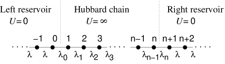
Figure 1: Hubbard chain with sites $j$ coupled to electron reservoirs $L$ and $R$. The hopping amplitude $\lambda_{j}$ varies along the chain and there is a repulsive on-site interaction $U$.

The system we consider is shown in Fig. 1. The sites of the infinite-$U$ Hubbard chain are labeled $j=1,\ldots,n$. The Hubbard chain is coupled to two noninteracting leads, with sites $j\leq 0$ and $j>n$. We introduce operators $\psi_{j\sigma}$ that annihilate an electron with spin $\sigma$ on site $j$ in the leads and $c_{j}$ that annihilate a hole at position $j$ in the Hubbard chain. The spin index $\sigma$ takes the values $1,\ldots,2S+1$. We also introduce operators $S_{{\rm L}\sigma}^{\dagger}$ and $S_{{\rm R}\sigma}^{\dagger}$ that add a spin $\sigma$ to the left and right of the spin configuration of the Hubbard chain, respectively. Our model Hamiltonian then reads

$$H = H_{\rm lead}+H_{\rm chain}+H^{\prime},$$ (1)

with

$$H_{\rm lead} = \lambda\sum_{\sigma}\left[\sum_{j<0}\psi^{\dagger}_{j\sigma}\psi_{j+1\sigma}+\sum_{j>n}\psi^{\dagger}_{j\sigma}\psi_{j+1\sigma}\right]+\mbox{h.c.}$$

$$H_{\rm chain} = \sum_{j=1}^{n-1}\lambda_{j}c^{\dagger}_{j}c_{j+1}+\mbox{h.c.}$$

$$H^{\prime} = \sum_{\sigma}\left(\lambda_{0}\psi_{0\sigma}^{\dagger}c_{1}^{\dagger}S^{{\phantom{\dagger}}}_{{\rm L}\sigma}+\lambda_{n}\psi_{n+1\sigma}^{\dagger}c_{n}^{\dagger}S^{{\phantom{\dagger}}}_{{\rm R}\sigma}\right)+\mbox{h.c.},$$

where we allowed for spatial variations of the hopping amplitude $\lambda_{j}$ of the Hubbard chain.

Moments of the number $\Delta N_{\sigma}=N_{\sigma}(\tau)-N_{\sigma}(0)$ of spin $\sigma$ electrons that are transported through the chain during a time $\tau$ can be obtained from the generating function

$${\cal Z}(\{\xi_{\sigma}\})={\rm Tr}\,e^{-i\xi N}\,e^{-iH\tau}\,e^{i\xi N}\,\rho\,e^{iH\tau}.$$ (2)

Here $\rho$ is the initial density matrix of the conductor and $\xi N$ abbreviates $\sum_{\sigma}\xi_{\sigma}N_{\sigma}$ with $N_{\sigma}=\sum_{j\leq 0}\psi^{{\dagger}}_{j\sigma}\psi^{{\phantom{\dagger}}}_{j\sigma}$. For large $\tau$, ${\cal Z}$ generates zero-frequency (spin) current correlators upon differentiation. We rewrite ${\cal Z}$ as

$${\cal Z}(\{\xi_{\sigma}\})={\rm Tr}\,e^{-iH_{\xi}\tau}\,\rho\,e^{iH\tau},$$ (3)

where $H_{\xi}=\exp({-i\xi N})H\exp({i\xi N})$. $H_{\xi}$ is obtained from $H$ by the substitution $\psi_{j\sigma}\to e^{i\xi_{\sigma}}\psi_{j\sigma}$ for $j\leq 0$. Since the Hamiltonian (1) is quadratic in the fermions, the lead fermions may be integrated out, so that the generating function ${\cal Z}$ takes the form

$${\cal Z}(\{\xi_{\sigma}\}) = \left\langle T_{\rm c}\exp\left[-i\lambda_{0}^{2}\int_{\rm c}dt_{1}dt_{2}\sum_{\sigma}S^{\dagger}_{{\rm L}\sigma}(t_{1})c_{1}(t_{1})G_{{\rm L}\sigma\xi}(t_{1},t_{2})c^{\dagger}_{1}(t_{2})S^{{\phantom{\dagger}}}_{{\rm L}\sigma}(t_{2})\right.\right.$$ (4)

$$\hphantom{\left\langle T_{\rm c}\exp\left[\vphantom{\int}\right.\right.}\left.\left.\mbox{}\!\!\!\!-i\lambda_{n}^{2}\int_{\rm c}dt_{1}dt_{2}\sum_{\sigma}S^{\dagger}_{{\rm R}\sigma}(t_{1})c_{n}(t_{1})G_{{\rm R}\sigma}(t_{1},t_{2})c^{\dagger}_{n}(t_{2})S^{{\phantom{\dagger}}}_{{\rm R}\sigma}(t_{2})\right]\right\rangle_{\rm chain},$$

where c denotes the Keldysh contour, $G_{{\rm L}}$ and $G_{{\rm R}}$ are Keldysh Green functions for the sites $0$ and $n+1$, respectively, and the averaging brackets $\langle\ldots\rangle_{\rm chain}$ represent an average with respect to the Hamiltonian $H_{\rm chain}$ of the uncoupled Hubbard chain. Using matrix notation in Keldysh space, one has $G_{{\rm L}\sigma\xi}=e^{i\xi_{\sigma}\tau_{3}/2}G_{{\rm L}\sigma}e^{-i\xi_{\sigma}\tau_{3}/2}$, where $\tau_{3}$ is the third Pauli matrix in Keldysh space.

The first limit in which exact results can be obtained is that of reservoirs with a large bandwidth $\lambda\to\infty$ that are completely filled with electrons on the left and completely empty on the right side of the chain. In that case, the reservoir Green functions $G_{{\rm L}}$ and $G_{{\rm R}}$ take a particularly simple form,

$$G_{{\rm L}}(t,t^{\prime}) = \frac{2i}{\lambda}\delta_{\lambda}(t-t^{\prime})\left(\begin{array}[]{cc}\theta(t^{\prime}-t)&1\\ 0&\theta(t-t^{\prime})\end{array}\right),$$ (7)

$$G_{{\rm R}}(t,t^{\prime}) = -\frac{2i}{\lambda}\delta_{\lambda}(t-t^{\prime})\left(\begin{array}[]{cc}\theta(t-t^{\prime})&0\\ 1&\theta(t^{\prime}-t)\end{array}\right),$$ (10)

where $\delta_{\lambda}$ is an approximation to a Dirac delta-function with width $1/\lambda$. In order to be able to take the limit $\lambda\to\infty$ while having a finite transport current we assume that the bandwidth of the chain is adiabatically reduced. We assume that $\lambda_{j}=\lambda$ for $j$ close to the boundaries of the Hubbard chain at $j=1$ and $j=n$, and that $\lambda_{j}$ is adiabatically reduced to a value $\lambda_{j}=\lambda_{\rm r}\ll\lambda$ in the center of the chain, $j\simeq n/2$.

Below, we will argue that, in this limit, one may make the following substitutions in the exponent of Eq. (4),

$$\sum_{\sigma}S_{{\rm L}\sigma}^{\dagger}(t_{1})G_{{\rm L}\sigma\xi}(t_{1},t_{2})S^{{\phantom{\dagger}}}_{{\rm L}\sigma}(t_{2}) \to \sum_{\sigma}G_{{\rm L}\sigma\xi}(t_{1},t_{2}),$$

$$\sum_{\sigma}S_{{\rm R}\sigma}^{\dagger}(t_{1})G_{{\rm R}\sigma}(t_{1},t_{2})S^{{\phantom{\dagger}}}_{{\rm R}\sigma}(t_{2}) \to G_{{\rm R}\sigma}(t_{1},t_{2}).$$ (11)

After these replacements, the generating function ${\cal Z}$ is readily calculated, and we find

$$\ln{\cal Z}=\frac{\tau}{h}\int_{-2\lambda_{\rm r}}^{2\lambda_{\rm r}}{d\omega\ln\left[1+\frac{T(\omega)}{2S+1}\sum_{\sigma}{(e^{i\xi_{\sigma}}}-1)\right]},$$ (12)

where, for $\lambda_{n}=\lambda$,

$$T(\omega)=\frac{(2S+1)|\lambda_{0}|^{2}(4\lambda^{2}-\omega^{2})}{(\lambda^{2}+(2S+1)|\lambda_{0}|^{2})^{2}-(2S+1)|\lambda_{0}|^{2}\omega^{2}}.$$ (13)

(We set $\lambda_{n}=\lambda$ to simplify the expressions reported here; it is not essential for the calculation.) The function $T(\omega)$ reaches its maximum $T^{\rm max}(\omega)=1$ for $\lambda_{0}=\lambda/\sqrt{2S+1}$ arti . While the maximum current in the corresponding wire without interactions would be $I^{\rm max}_{\rm n}=-4(2S+1)\lambda_{\rm r}\,e/h$, Eq. (12) implies for the interacting case

$$I^{\rm max}=\frac{1}{2S+1}I^{\rm max}_{\rm n}.$$ (14)

Hence, for electrons with spin $S=1/2$ interactions reduce the maximal charge current by a factor of $2$. This signals a reduction of the conductance of the wire from $2e^{2}/h$ to $e^{2}/h$, as in the infinitely long system. Every spin component carries an equal part of that total charge current independently of the chosen spin quantization direction: the electrons in the wire are not spin-polarized. This absence of spin-polarization in the wire is also reflected in fluctuations of the spin currents through the wire. At maximal transmission we find for their variance

$$\mbox{var}\,\Delta N_{\sigma}=\frac{4\lambda_{\rm r}\tau}{h}\frac{2S}{(2S+1)^{2}}.$$ (15)

In contrast, the charge current is noiseless in this case:

$${\rm var}\,\left(\sum_{\sigma}\Delta N_{\sigma}\right)=0.$$ (16)

Our model therefore indeed exemplifies a mechanism of conductance reduction through electron-electron interactions that does not introduce any shot noise. Instead of blocking the transport of electrons with certain spin directions by spin-polarizing the wire, this mechanism reduces the conductance by limiting the density of conduction electrons to the spinless case while allowing them to have arbitrary spin.

We now discuss the justification of the replacements (11). This is done by expanding the exponential of Eq. (4) in powers of $\lambda_{0}$ and $\lambda_{n}$. For simplicity we specialize to the case $\lambda_{0}=\lambda_{n}/\sqrt{2S+1}$. Since the spin operators $S^{{\phantom{\dagger}}}_{{\rm L}\sigma}$ and $S_{{\rm L}\sigma}^{\dagger}$ have no dynamics in the absence of coupling to the reservoirs, the time dependence of the spin operators is not important; only their order in the contour-ordered expression (4) matters. To second order in $\lambda_{n}$, the causal structure of the reservoir Green function $G_{\rm L}$ is such that $S^{{\phantom{\dagger}}}_{{\rm L}\sigma}(t_{2})$ always appears to the left of $S_{{\rm L}\sigma}^{\dagger}(t_{1})$. Since $S^{{\phantom{\dagger}}}_{{\rm L}\sigma}S_{{\rm L}\sigma}^{\dagger}=1$, the first substitution rule (11) follows. Similarly, the causal structure of the reservoir Green function $G_{\rm R}$ is such that $S^{{\phantom{\dagger}}}_{{\rm R}\sigma}(t_{2})$ always appears to the right of $S_{{\rm R}\sigma}^{\dagger}(t_{1})$. The operator product $S^{\dagger}_{{\rm R}\sigma}S^{{\phantom{\dagger}}}_{{\rm R}\sigma}=1$ if the right-most electron of the Hubbard chain has spin $\sigma$, and $S^{\dagger}_{{\rm R}\sigma}S^{{\phantom{\dagger}}}_{{\rm R}\sigma}=0$ otherwise. Hence $\sum_{\sigma}S^{\dagger}_{{\rm R}\sigma}S^{{\phantom{\dagger}}}_{{\rm R}\sigma}=1$, and the second substitution rule of Eq. (11) follows.

We next prove the substitution rules (11) for higher orders in $\lambda_{n}$. A key ingredient in this will be the locality of the reservoir Green functions which groups spin operators into ordered pairs that act almost simultaneously. This essentially decouples different spin operator pairs and the rules (11) follow like at first order in $\lambda_{n}$. To show this we decompose the hole annihilation operators $c_{j}=c_{j,e}+c_{j,t}$ into a contribution $c_{j,e}$ from evanescent states of the chain at energies $\epsilon\geq 2\lambda_{\rm r}$ and a contribution $c_{j,t}$ from transmitting states with $\epsilon<2\lambda_{\rm r}$. In any term of an expansion of ${\cal Z}$ in powers of $\lambda_{n}$ we first contract all hole operators $c_{j,e}$ into pairs using Wick’s theorem. This produces sequences of the form

$$D_{{\rm L};l} = \int_{\rm c}dt_{2}\ldots dt_{l-1}\,c^{\phantom{\dagger}}_{1,t}(t_{1})S^{\dagger}_{\rm L}(t_{1})G_{{\rm L}\xi}(t_{1},t_{2})$$ (17)

$$\mbox{}\times S_{\rm L}^{\phantom{\dagger}}(t_{2})g_{e}(t_{2},t_{3})\ldots S_{\rm L}^{\phantom{\dagger}}(t_{l})c^{\dagger}_{1,t}(t_{l}),$$

consisting of spin operators and two transmitting hole operators $c_{1,t}$, connected by Green functions for lead and chain fermions. All evanescent hole states on the left side of the chain are unoccupied because of their proximity to the left reservoir, so that the evanescent hole Green function $g_{e}$ has the same causal structure as $G_{{\rm R}}$, cf. Eq. (10). This assures that after time ordering all spin operators in such sequences are grouped in pairs $S^{\dagger}_{\rm L}(t_{i})G_{{\rm L}\xi}(t_{i},t_{i+1})S_{\rm L}^{\phantom{\dagger}}(t_{i+1})$ originating from the same reservoir Green function with no other spin operator $S^{\phantom{\dagger}}_{\rm L}$ or $S^{\dagger}_{\rm L}$ acting in between. The substitution rules (11) follow then for such sequences as before for a single pair. The same arguments hold for the right side of the chain. It remains to contract the operators $c_{j,t}$ at the beginning and at the end of sequences $D_{{\rm L},{\rm R},l}$ of the form (17). Here, nothing prevents spin operators of one sequence $D_{{\rm L},{\rm R};k}$ to occur in time between operators $S^{\dagger}_{\rm L}(t_{i})G_{{\rm L}\xi}(t_{i},t_{i+1})S_{\rm L}^{\phantom{\dagger}}(t_{i+1})$ in another sequence $D_{{\rm L},{\rm R};l}$. Such events cause corrections to the generating function calculated with the substitution rules (11). However, because of the locality of the lead Green functions $G$, such corrections occur only in time intervals of length $1/\lambda$. This is much shorter than the range of the integrals over the times $t_{1}$ and $t_{l}$ of sequences $D_{{\rm L},{\rm R};l}$, which is set by the time scale $1/\lambda_{\rm r}$ on which the Green functions of transmitting hole states vary. Therefore, corrections are of order $\lambda_{\rm r}/\lambda$, and can be neglected in our limit $\lambda_{\rm r}/\lambda\to 0$.

To make this argument rigorous one needs to estimate the corrections to all terms in an expansion of the cumulant generating function $\ln{\cal Z}$. Only “connected” diagrams contribute to $\ln{\cal Z}$. Spin operators in its expansion can be connected either by fermion Green functions or by deviations from the operator ordering underlying the substitution rules (11). As we argued above, the corrections to diagrams where all spin operators are connected by Green functions are of order $\lambda_{\rm r}/\lambda$. Let us now estimate the correction arising from diagrams that are connected because of deviations from the ordering underlying the rules (11). Hereto, note that a product of two sequences $j$ and $k$ of spin operators that are connected cyclically by fermion Green functions only within themselves still contributes to $\ln{\cal Z}$ if a spin operator of one of the sequences acts in between an operator pair $S^{\dagger}_{\rm L}(t_{i})G_{{\rm L}\xi}(t_{i},t_{i+1})S_{\rm L}^{\phantom{\dagger}}(t_{i+1})$ of the other sequence. When uncorrelated the two subsequences are of order $\tau(\lambda_{n}/\lambda)^{2n_{j}}\lambda_{\rm r}$ and $\tau(\lambda_{n}/\lambda)^{2n_{k}}\lambda_{\rm r}$, respectively, where $n_{m}$ is the number of reservoir Green functions $G$ contained in sequence $m$. Correlations between the subsequences occur for the time $1/\lambda$ over which spin operators interfere and the corresponding correction is therefore of order $\tau(\lambda_{n}/\lambda)^{2n_{j}+2n_{k}}(\lambda_{\rm r}/\lambda)\lambda_{\rm r}$. This is of the same order as the correction to a sequence connected entirely by Green functions at the same order in $\lambda_{n}$. This correspondence holds for diagrams with an arbitrary number of connections by spin operators. We now take into account that every one of the discussed sequences contains many pairs of spin operators that can interfere with other operators. We estimate that at order $(\lambda_{\rm r}/\lambda)^{k}$ the correction $\Delta_{k;l}$ to a term of order $2l$ in $\lambda_{n}$ in the expansion of $\ln{\cal Z}$ is of relative order

$$\Delta_{k;l}\sim\left(\begin{array}[]{cc}2l\\ k\end{array}\right)\left(\frac{\lambda_{n}}{\lambda}\right)^{2l}\left(\frac{\lambda_{\rm r}}{\lambda}\right)^{k}.$$ (18)

Summing up these contributions one finds that the total correction to $\ln{\cal Z}$ is of relative order $\epsilon\ll 1$ if $\lambda_{n}/\lambda<\exp(\lambda_{\rm r}\ln\epsilon/\lambda\epsilon)$. In the limit $\lambda_{\rm r}/\lambda\to 0$ the substitution rules Eq. (11) are therefore justified for arbitrarily good transmission $T<1$, where $T\to 1$ in the limit $\lambda_{n}\to\lambda$.

The second limit in which exact results can be obtained is in the presence of additional spin relaxation processes in the Hubbard chain. To the Hamiltonian (1) we add a random time-dependent magnetic field that causes spin memory to be lost at a rate $\gamma_{S}$. In the limit $\gamma_{S}\gg|\lambda|$ our model is again exactly solvable, now both in and out of equilibrium and without assumptions about $\lambda_{j}$. To demonstrate this we consider a wire with a constant $\lambda_{j}=\lambda$. Every operator $S^{{\phantom{\dagger}}}_{{\rm R}\sigma}(t)$ or $S^{{\phantom{\dagger}}}_{{\rm L}\sigma}(t)$ in an expansion of ${\cal Z}$ is nonvanishing only if $\sigma$ equals the state of the last or first spin of the Hubbard chain at time $t$. In the limit $\gamma_{S}\gg|\lambda|$ any memory of the state of the spin put into the chain by previous actions of the operators $S^{{\dagger}}_{{\rm R}\sigma}$ and $S^{{\dagger}}_{{\rm L}\sigma}$ is immediately erased by relaxation processes. After averaging over the random magnetic field, every term from the exponent of Eq. (4) contributes therefore only for one random spin state $\sigma$. This allows us again to represent ${\cal Z}$ by an expression of the form of Eq. (4) without spin operators. To obtain the generating function of charge currents we set $\xi_{\sigma}=e\xi$ and evaluate Eq. (4) with the substitutions

$$\sum_{\sigma}S_{\mu\sigma}^{\dagger}(t_{1})G_{\mu\sigma}(t_{1},t_{2})S_{\mu\sigma}(t_{2}) \to G_{\mu\sigma}(t_{1},t_{2}),$$ (19)

$\mu\in\{{\rm L},R\}$, to find that

$$\ln{\cal Z} = \frac{\tau}{h}\int_{-2\lambda}^{2\lambda}{d\omega\,\ln\left\{1+T(\omega)\right.}$$ (20)

$$\!\!\!\!\!\!\!\!\!\!\!\!\!\!\!\!\!\!\!\!\!\!\!\!\!\!\!\!\!\!\!\!\left.\mbox{}\;\left[f_{L}(1-f_{R})\left(e^{ie\xi}-1\right)+f_{R}(1-f_{L})\left(e^{-ie\xi}-1\right)\right]\right\}.$$

Here, $T(\omega)$ is given by Eq. (13) evaluated at $S=0$ and $f_{\mu}$ are the occupation numbers of reservoir states. $T(\omega)$ now reaches its maximum $T^{\rm max}(\omega)=1$ for $\lambda_{0}=\lambda_{n}=\lambda$. Charge transport through the chain becomes indistinguishable from that through a noninteracting single-channel conductor for spinless fermions. We again find noiseless charge current at zero temperature while the conductance is reduced to $e^{2}/h$, a factor $2S+1$ smaller than its noninteracting value. This shows that the discussed mechanism of noiseless conductance reduction works also in equilibrium and for a not fully occupied electronic band. In fact, the condition for the spin relaxation rate $\gamma_{S}$ may be relaxed for a wire with an almost empty conduction band. For a long wire, $n\gg\lambda^{2}/\Delta\lambda\gamma_{S}$, Eq. (20) can be shown to hold also in the experimentally more relevant situation that the spin decoherence rate in the wire exceeds the range $\Delta\lambda$ of energies for which electronic states are appreciably occupied, $\gamma_{S}\gg\Delta\lambda$ unpub .

In conclusion, by studying two exactly solvable limits of a Coulomb Tonks gas coupled to bulk leads, we have shown that strong electron-electron interactions can lead to a noiseless conductance reduction without spin-polarization. One may speculate that the same mechanism could be operative also in other parameter regimes. As such it appears to be a plausible alternative interpretation of the measurement of a suppression of shot noise at the 0.7-plateau of quantum point contacts reported in Refs. noise . Further evidence for the studied mechanism could be found in similar measurements on carbon nanotubes, to which our model applies more directly Fog05 . Such measurements could moreover put an important constraint on theories of the anomalous conductance reduction observed in some quantum wires 07 ; CN .

This work was supported by the NSF under grant no. DMR 0334499 and by the Packard Foundation.

References

- (1) Ya. M. Blanter and M. Büttiker, Phys. Rep. 336, 1 (2000).
- (2) B. J. van Wees et al., Phys. Rev. Lett. 60, 848 (1988).
- (3) D. A. Wharam et al., J. Phys. C 21, L209 (1988).
- (4) M. I. Reznikov et al., Phys. Rev. Lett. 75, 3340 (1995); A. Kumar et al., Phys. Rev. Lett. 76, 2778 (1996).
- (5) P. Roche et al., Phys. Rev. Lett. 93, 116602 (2004); N. Y. Kim et al., cond-mat/0311435.
- (6) M. M. Fogler, Phys. Rev. B 71, 161304(R) (2005).
- (7) V. V. Cheianov and M. B. Zvonarev, Phys. Rev. Lett. 92 176401 (2004); G. A. Fiete and L. Balents, Phys. Rev. Lett. 93, 226401 (2004); G. A. Fiete, K. Le Hur, and L. Balents, cond-mat/0505186.
- (8) J. Biercuk et al., Phys. Rev. Lett. 94, 026801 (2005).
- (9) K. A. Matveev, Phys. Rev. Lett. 92, 106801 (2004); K. A. Matveev Phys. Rev. B 70, 245319 (2004).
- (10) D. J. Reilly et al., Phys. Rev. B 63, 121311(R) (2001); K. J. Thomas et al., Phys. Rev. B 61, 13 365(R) (2000).
- (11) D. L. Maslov and M. Stone, Phys. Rev. B 52, 5539(R) (1995); V. V. Ponomarenko, Phys. Rev. B 52, 8666(R) (1995); I. Safi and H. J. Schulz, Phys. Rev. B 52, 17 040(R) (1995).
- (12) V. V. Ponomarenko and N. Nagaosa, Phys. Rev. B 60, 16865 (1999).
- (13) The discontinuous coupling at maximal transmission is an artifact of our model. It would be smoothed out if interactions were decreased adiabatically towards the reservoirs.
- (14) M. Kindermann, unpublished.