Superfluid-Insulator Transitions on the Triangular Lattice

Abstract

We report on a phenomenological study of superfluid to Mott insulator transitions of bosons on the triangular lattice, focusing primarily on the interplay between Mott localization and geometrical charge frustration at 1/2-filling. A general dual vortex field theory is developed for arbitrary rational filling factors $f$, based on the appropriate projective symmetry group. At the simple non-frustrated density $f=1/3$, we uncover an example of a deconfined quantum critical point very similar to that found on the half-filled square lattice. Turning to $f=1/2$, the behavior is quite different. Here, we find that the low-energy action describing the Mott transition has an emergent nonabelian $SU(2)\times U(1)$ symmetry, not present at the microscopic level. This large nonabelian symmetry is directly related to the frustration-induced quasi-degeneracy between many charge-ordered states not related by microscopic symmetries. Through this “pseudospin” $SU(2)$ symmetry, the charged excitations in the insulator close to the Mott transition develop a skyrmion-like character. This leads to an understanding of the recently discovered supersolid phase of the triangular lattice XXZ modelMelko05 ; Damle05 ; Troyer05 as a “partially melted” Mott insulator. The latter picture naturally explains a number of puzzling numerical observations of the properties of this supersolid. Moreover, we predict that the nearby quantum phase transition from this supersolid to the Mott insulator is in the recently-discovered non-compact CP¹ critical universality class.Lesik   A description of a broad range of other Mott and supersolid states, and a diverse set of quantum critical points between them, is also provided.

I Introduction

Theoretical interest in quantum phase transitions from superfluid to Mott insulating states of bosons has recently been revived by their experimental realization in cold atoms trapped in an optical lattice.Greiner Extensions of these experiments are expected to soon provide a great variety of real life toy models, where theoretical scenarios for such phase transitions can be tested.Demler03 ; Zoller04 ; Zoller05 For the condensed matter community, such transitions are interesting in their own right, but also provide a simpler context in which some aspects of Mott conducting-insulating transitions of electrons can be explored. A better understanding of such Mott criticality generally may help to explain mysteries in various strongly correlated materials, from heavy fermion metals livrefs to cuprate superconductors,cuprefs in which Mott criticality may plausibly be argued to play a key role.

An exciting theoretical development in the field has been the discovery that some quantum phase transitions require a fundamentally new description, not based on the now-standard Landau’s concept of an order parameter. Instead, such quantum critical points (QCPs) are described in terms of emergent degrees of freedom, not present in either phase and appearing due to certain special dynamically generated low-energy symmetries at the critical point.dcprefs An interesting consequence of the emergent low-energy symmetry of the critical point is the near-degeneracy of “competing ordered” states unrelated by any microscopic symmetry (but unified with one another by the emergent one) in the neighborhood of the quantum phase transition. There is, at present, unfortunately, no general way to a priori identify the appropriate emergent degrees of freedom, should they exist, for any putative quantum critical point.

In the particular context of two-dimensional bosonic superfluid-insulator transitions, a general non-Landau-Ginzburg-Wilson (non-LGW) framework has recently been proposed in Ref. Balents04, (and see Ref. ykis, for a pedagogical review), and carried out explicitly on the square lattice. In particular, the Mott transition can be described in terms of the vortex excitations of the superfluid. In a two dimensional superfluid, vortices are point-like “particles” whose creation/annihilation operators can be used to construct a quantum field theory. The vortices being non-local topological objects, these vortex fields are, however, not themselves order parameters in the LGW sense. The non-locality is manifested by the presence of a (non-compact) $U(1)$ gauge field, to which the vortex fields are coupled in the “dual” vortex field theory. This formulation is general because it is based on the excitations of the superfluid, which is a stable and apparently featureless (i.e. without broken symmetry apart from off-diagonal long range order) state at any boson density. Nevertheless, it was shown in Ref. Balents04, that the vortices exhibit a subtle quantum order which is sensitive to the boson density $f$ (per unit cell of the lattice). In particular, at non-integral $f$, the vortices form non-trivial multiplets transforming under a projective symmetry group (PSG - technically, a projective representation of the lattice space group). The Lagrange density for the vortex field theory therefore takes the general form

$${\cal L} = \sum_{\ell=0}^{N}\left[|(\partial_{\mu}-iA_{\mu})\varphi_{\ell}|^{2}+s|\varphi_{\ell}|^{2}\right]+{\cal L}_{\rm int}[\{\varphi_{\ell}\}]$$ (1)

$$+\frac{1}{2e^{2}}(\epsilon_{\mu\nu\lambda}\partial_{\nu}A_{\lambda})^{2},$$

where $\varphi_{\ell}$ with $\ell=1\ldots N$ are vortex fields for the $N$ members of the multiplet ($N$ depends upon $f$ – see Sec. II), and $A_{\mu}$ is the dual $U(1)$ gauge field. Quartic and higher order terms are contained in ${\cal L}_{\rm int}$, the structure of which is dictated by the PSG. The Mott transition is captured by Eq.(1) in a simple way. The ground state of $s>0$ corresponds to the vacuum of vortices – flux is expelled from the system, so this is a superfluid. In the $s<0$ phase, at least one of the vortex flavors will condense, and the gauge fields will acquire a gap by the Higgs mechanism. This is indicative of a charge gap, and describes an incompressible Mott insulating phase.

Transformations within the $\varphi_{\ell}$ multiplet comprise the emergent symmetry operations of the “deconfined” quantum critical point. This structure has an important physical consequence as well: it naturally and unavoidably leads to (particular) broken spatial symmetries in the Mott state. A mean-field analysis of the vortex field theory predicts a direct superfluid to Mott transition, as well as the nature of the charge ordering in the Mott phase.

In this paper, we extend this vortex field theory approach to describe superfluid to Mott insulator transitions of bosons on the triangular lattice (hexagonal lattice in proper crystallographic nomenclature) at fractional boson fillings $f=p/q$, with $p,q$ relatively prime integers. We focus particularly on the most interesting examples, $f=1/2$ and $f=1/3$. The $1/2$-filling case introduces a new ingredient not present on the square lattice: geometrical frustration. Here we refer to “charge frustration” of the ordering of localized boson configurations in the presence of short-range repulsive interactions. A consequence – or perhaps definition – of such geometrical frustration is the exact or near degeneracy of many distinct ordered states. The similarity of this property with the emergent near-degeneracy of competing orders near a deconfined quantum critical point suggests a possible link between the two phenomena. This connection indeed appears to be borne out by the analysis in this paper.

In the simplest classical models of frustration, the degeneracy amongst low-energy states is not only large but macroscopic (i.e. with an entropy proportional to the sample volume). This classical degeneracy, when lifted by quantum fluctuations, may produce unusual ground states. A number of very recent papersMelko05 ; Damle05 ; Troyer05  have investigated the system of hardcore bosons with nearest-neighbor interactions (which can be mapped to a spin-$1/2$ XXZ model) on the triangular lattice near half-filling. This realizes such approximately classical frustration in the limit of very strong near-neighbor repulsion. These works demonstrated that in this system the lifting of the macroscopic classical degeneracy results in an unusual supersolid ground state, which we denote SS3 because of its 3-sublattice structure. This “order by disorder” mechanism is very different from the “conventional” (theoretically!) picture of supersolidity, via a condensation of vacancies and/or interstitials in an ordered solid.supersolid

Since the above studies clarified that such Mott states do not occur in the simplest nearest-neighbor interaction model, it is apparent that microscopically, longer-range interactions, possibly including ring-exchange,Sandvik02 are necessary to observe these transitions in a microscopic model. Finding simple interactions that produce nontrivial insulating ground states on the triangular lattice is an important and difficult problem, that will likely require sophisticated numerical methods. We will not address this issue here (but see the Discussion, Sec. V).

Our phenomenological vortex field theory, on the contrary, describes universal aspects (independent of microscopic realization) of Mott insulating, superfluid, and other states, and the transitions between them. As for the square lattice case, a mean-field analysis predicts a direct superfluid-Mott transition, with a diverse set of Mott insulating phases. Also like the square lattice, the vortex field theory has an enhanced emergent symmetry at the critical point, a hallmark of deconfined criticality. A significant difference from these prior examples of deconfined criticality, however, is that, in the frustrated case, $f=1/2$, the emergent symmetry is nonabelian, containing an $SU(2)$ “pseudospin” subgroup. The much larger (than in non-frustrated cases) emergent symmetry can be understood physically as symptomatic of the larger near-degeneracies present in this case due to frustration.

Remarkably, going beyond the mean-field analysis of the vortex field theory, our approach connects very nicely to the supersolid phase of the XXZ model. Indeed, the supersolid order parameter – describing the growth of the supersolid state out of the featureless superfluid – appears in a particularly simple form in the vortex variables. Moreover, our approach reveals an alternative view of the supersolid, as a partially-melted “parent” Mott insulating state, with “quantum disordered” pseudospin. This loss of pseudospin order simultaneously with the onset of superfluidity is possible because, as we show, the pseudospin skyrmion excitation of the Mott insulator carries physical boson charge. The supersolid may thereby also be viewed as a condensate of these skyrmions. Furthermore, this picture leads directly to the prediction that the Mott insulator to SS3 transition is described by the recently discovered Non-Compact CP¹ (NCCP¹) quantum critical universality class.Lesik  This transition describes the quantum disordering of a pseudospin vector ${\bf S}$ (the order parameter for the additional solid order of the Mott state) in $2+1$ dimensions, when “hedgehog” instantons are absent in space-time. These hedgehog events correspond precisely to processes which change the skyrmion number, and are therefore prohibited by charge conservation in this case.

The paper is organized as follows. In Sec.II we develop the dual vortex theory for the triangular lattice at a general rational filling. We derive the PSG transformations of the degenerate low energy vortex modes and discuss some of their general properties. In Sec. III we apply this theory to the two cases $f=1/3$ and $f=1/2$, and discuss the resulting Mott states that are obtained by a mean field analysis of the vortex field theory. In Sec. IV we present a “hard-spin” formulation of the vortex action, which enables a study of its phases and transitions beyond mean field theory. We discuss the new phases which arise, notably supersolids, the elementary excitations of the different states, and the transitions amongst them. This includes notably the SS3 phases and the NCCP¹ transitions between them and their parent Mott insulator. We conclude with a discussion in Sec. V of a more microscopic physical picture for the most interesting Mott and supersolid states at half-filling, the connection to the recent studies of the XXZ model, and the prospects for observing more of the physics in this paper in related models. A number of appendices provide useful details of various technical results.

II Continuum dual vortex theory

As discussed in the introduction, our aim is to derive a field theoretic description of the vicinity of a superfluid to Mott insulator transition, in terms of the vortex excitations of the superfluid state. As is well-known, lattice models of bosons can indeed be reformulated in vortex variables on the dual lattice, a technique called duality. As detailed for instance in Ref. ykis, (and references therein), this can in principle be carried out exactly for any lattice boson Hamiltonian, e.g. Bose-Hubbard models, XXZ models, etc. Unfortunately, this exact mapping does not lead to a particularly tractable limit of the vortex theory, and it is therefore difficult to extract quantitative predictions directly from the lattice vortex theory.

Fortunately, we can avoid this difficulty in addressing our stated goal of understanding universal phenomena in the vicinity of the superfluid-Mott quantum critical point. For this purpose, we need not specify any particular microscopic boson model. Instead, we will illustrate the calculations through the use of a very simple lattice vortex theory, which is chosen to have the same spatial symmetries as the physical triangular lattice, and to exhibit a superfluid to Mott insulation transition. The universal properties of interest will coincide with those of more physical microscopic boson models.

In the Euclidean vortex coherent-state path integral formulation in which we work, the lattice vortex action is

$$S = -t_{v}\sum_{a\mu}[\psi^{*}_{a}e^{-iA_{a\mu}}\psi_{a+\mu}+c.c.]$$ (2)

$$+ \sum_{a}[s|\psi_{a}|^{2}+u|\psi_{a}|^{4}]$$

$$+ \frac{1}{2e^{2}}\sum\left(\epsilon_{\mu\nu\lambda}\Delta_{\nu}A_{a\lambda}-2\pi f\delta_{\mu\tau}\right)^{2}.$$

Here $a$ labels sites of the dual 2+1-dimensional uniformly stacked honeycomb lattice, with the vertical direction being the imaginary time direction $\tau$, and $\mu$ is summed over nearest-neighbor links (3 at $120$ degrees connecting spatial neighbors and a fourth along the imaginary time direction). The action is written in terms of the complex vortex field $\psi_{a}$ (and its conjugate $\psi_{a}^{*}$) which annihilates (creates) unit vorticity, as well as a dual gauge field $A_{a\mu}$. The physical meaning of the gauge field $A_{a\mu}$ is that its curl gives ($2\pi$ times) the bosonic 3-current density, and importantly, the temporal component of the current density is ($2\pi$ times) the charge density. For a bosonic system with density $f$ bosons per site, we must therefore enforce the condition that $2\pi f$ flux on average passes through each hexagonal plaquette of the honeycomb lattice. We will assume the filling to be rational $f=p/q$, where $p$ and $q$ are relatively prime integers, and will mostly concentrate on the two cases $f=1/2,1/3$. Physically, $t_{v}$ represents a vortex hopping amplitude, $s$ and $u$ represent short-range vortex “core” energies and interactions, and $e^{2}$ represents the strength of the dual electromagnetic field fluctuations (it is roughly proportional to the local superfluid density away from the Mott quantum critical point).

Figure 1: Dual honeycomb lattice. Reflection axes $d_{1}$ and $d_{2}$ are shown by dashed lines.

We may think of the parameter $s$ in Eq.(2) as driving the superfluid-insulator transition. Large positive $s$ corresponds to the superfluid phase, in which vortices are gapped, and large negative $s$ corresponds to the set of possible insulating phases, in which vortices are condensed. It is convenient to think about the transition in Eq. (2) for small $e^{2}$, i.e. neglecting to a first approximation dual gauge fluctuations – they will however be restored at a later stage of analysis. In this limit we can treat the dual gauge field in a mean field approximation and take:

$$\epsilon_{\mu\nu\lambda}\Delta_{\nu}A_{a\lambda}=2\pi f\delta_{\mu\tau}.$$ (3)

As $s$ is decreased from large positive values, we expect an instability of the “vortex vacuum” when the energy of the lowest vortex excitation approaches zero – or equivalently, when the minimum eigenvalue of the quadratic form for $\psi_{a},\psi_{a}^{*}$ in Eq. (2) vanishes. To study the universal critical properties of the superfluid-insulator transition, it is sufficient to isolate these low-energy particles, which comprise the vortex multiplets discussed in the introduction. The continuum limit of Eq. (2) then consists of a set of vortex fields, each representing one of these minimum energy vortex particles. We will also take the trivial continuum limit of Eq.(2) in the temporal direction.

Because of the non-zero gauge flux through each spatial plaquette, the minimum energy multiplets are non-trivial. The form of the continuum action in this case is determined by the projective representation of the space group (PSG), Balents04 under which the vortex fields $\psi$ transform. To find it, we must work through the consequences of some specific gauge choice. As in Ref.Balents04, , we will choose the Landau gauge for $A_{a\mu}$. Namely, let

$${\bf a}_{1}=\hat{x},\,\,\,{\bf a}_{2}=-\frac{1}{2}\hat{x}+\frac{\sqrt{3}}{2}\hat{y},$$ (4)

be the two basis vectors of the honeycomb lattice, as shown in Fig.1 (note that the honeycomb lattice has two sites per unit cell). Coordinates will be specified, when explicit, in this basis, ${\bf r}=a_{1}{\bf a}_{1}+a_{2}{\bf a}_{2}$, with integer $a_{1},a_{2}$, and $a_{1}=a_{2}=0$ corresponding to a “type 1” site (see Fig. 1) of the dual honeycomb lattice. Landau gauge is

$$A_{ay}=2\pi fa_{1},$$ (5)

and $A_{a\mu}=0$ for all other directions; that is, only the gauge field on vertical links is chosen non-zero. The full PSG is generated by a set of unitary transformations of $\psi$, one for each generator of the lattice space group. For the triangular lattice, we choose the space group generators as two elementary lattice translations $T_{1},T_{2}$, a $2\pi/3$ rotation with respect to site $1$ in Fig. 1, $R_{2\pi/3}$, and two reflections, $I_{d_{1}},I_{d_{2}}$. The PSG transformations of the vortex fields, characterized by the unimodular complex number $\omega=e^{2\pi if}$, are then:

$$T_{1} : \left\{\begin{array}[]{lcl}\psi_{1}(a_{1},a_{2})&\rightarrow&\psi_{1}(a_{1}\!-\!1,a_{2})\omega^{a_{2}}\\ \psi_{2}(a_{1},a_{2})&\rightarrow&\psi_{2}(a_{1}\!-\!1,a_{2})\omega^{a_{1}+1}\end{array}\right.,$$ (8)

$$T_{2} : \left\{\begin{array}[]{lcl}\psi_{1}(a_{1},a_{2})&\rightarrow&\psi_{1}(a_{1},a_{2}\!-\!1)\\ \psi_{2}(a_{1},a_{2})&\rightarrow&\psi_{2}(a_{1},a_{2}\!-\!1)\end{array}\right.,$$ (11)

$$R_{2\pi/3} : \left\{\begin{array}[]{lcl}\psi_{1}(a_{1},a_{2})&\rightarrow&\psi_{1}(a_{2}\!-\!a_{1},-a_{1})\omega^{\frac{a_{1}(2a_{2}-a_{1}-1)}{2}}\\ \psi_{2}(a_{1},a_{2})&\rightarrow&\psi_{2}(a_{2}\!-\!a_{1},-a_{1}\!-\!1)\omega^{\frac{a_{1}(2a_{2}-a_{1}+1)}{2}}\end{array}\right.,$$ (14)

$$I_{d_{1}} : \left\{\begin{array}[]{lcl}\psi_{1}(a_{1},a_{2})&\rightarrow&\psi_{1}^{*}(-a_{2},-a_{1})\omega^{a_{1}a_{2}}\\ \psi_{2}(a_{1},a_{2})&\rightarrow&\psi_{2}^{*}(-a_{2}\!-\!1,-a_{1}\!-\!1)\omega^{a_{1}(a_{2}+1)}\end{array}\right.,$$ (17)

$$I_{d_{2}} : \left\{\begin{array}[]{lcl}\psi_{1}(a_{1},a_{2})&\rightarrow&\psi_{2}^{*}(a_{2},a_{1}\!-\!1)\omega^{a_{1}a_{2}}\\ \psi_{2}(a_{1},a_{2})&\rightarrow&\psi_{1}^{*}(a_{2}\!+\!1,a_{1})\omega^{a_{1}(a_{2}+1)}\end{array}\right..$$ (20)

For the special case $f=1/2$, in which we are principally interested, one usually considers in addition to these spatial symmetries, an extra particle-hole symmetry, which we denote $C$ for “charge conjugation”. This interchanges singly-occupied and empty sites on the direct lattice. In the spin language appropriate for hard-core bosons, this is just a $180^{\circ}$ rotation around the $x$ axis in spin space, which has the effect of an Ising transformation $S_{i}^{z}\rightarrow-S_{i}^{z}$ (and likewise for $S_{i}^{y}$). The XXZ model, and indeed any hard core boson model at $f=1/2$ with only pairwise interactions, possesses such a particle-hole symmetry. In the dual theory, this requires the action to be invariant under

$$C\,:\,\psi_{i}(a_{1},a_{2})\rightarrow\psi_{i}^{*}(a_{1},a_{2}),$$ (21)

and simultaneous sign change of the fluctuating part of the dual gauge field $A_{\mu}\rightarrow-A_{\mu}$.

The quadratic action of Eq. (2) in Landau gauge has a periodicity in real space of $q$ unit cells in the ${\bf a}_{1}$ direction, and one unit in the ${\bf a}_{2}$ direction (note that, of course, the physics itself has the full periodicity of the honeycomb (or underlying triangular direct) lattice). The eigenstates of the quadratic action can therefore be characterized by their quasimomenta in the corresponding reduced Brillouin zone. Specifically, we introduce the basis vectors of the reciprocal lattice,

$${\bf b}_{1}=\hat{x}+\frac{1}{\sqrt{3}}\hat{y},\,\,\,{\bf b}_{2}=\frac{2}{\sqrt{3}}\hat{y}.$$ (22)

Wavevectors will, when necessary, be specified by coordinates $(k_{1},k_{2})$, with ${\bf k}=k_{1}{\bf b}_{1}+k_{2}{\bf b_{2}}$ (reciprocal lattice vectors correspond to $k_{1},k_{2}$ being integral multiples of $2\pi$).

By applying the methods of Ref.Balents04, , one may readily find the minimum energy multiplet for arbitrary $p,q$, and their PSG transformations. Briefly, this is accomplished by Fourier transforming Eqs. (8) to obtain the PSG for general $\psi({\bf k})$ in momentum space – this is given in Appendix A – and using the non-commutative algebra of translations and rotations implicit in Eqs. (8) to generate a full set of eigenfunctions. One finds two cases. For $q$ odd, there are $q$ minima of the vortex dispersion, i.e. $N=q$ in Eq. (1). These occur at momenta

$${\bf k}_{\ell}=\left(0,2\pi f\ell\right),\,\,\,\ell=0,\ldots,q-1,$$ (23)

taking wavevectors ${\bf k}_{\ell}$ to lie in the reduced Brilloin zone $-\pi/q\leq k_{1}<\pi/q$ and $-\pi\leq k_{2}<\pi$. By contrast, for $q$ even, $N=2q$, and it is convenient to divide minima into two sets $\alpha=\pm 1\equiv\pm$, parameterizing $\ell=(1+\alpha)q/2+\sigma$, $\sigma=0\ldots q-1$. The vortex field operator $\varphi_{\alpha\sigma}$ then acts on eigenstates with the wavevector

$${\bf k}_{\alpha\sigma}=\left(\pi\alpha/3q,\pi\alpha/3q+2\pi f\sigma\right)$$ (24)

in the reduced Brillouin zone. For even $q$, therefore, Eq. (1) may be rewritten as

$${\cal L}_{0}^{even} = \sum_{\alpha=\pm}\sum_{\sigma=0}^{q-1}\left[|(\partial_{\mu}-iA_{\mu})\varphi_{\alpha\sigma}|^{2}+s|\varphi_{\alpha\sigma}|^{2}\right]$$ (25)

$$+ \frac{1}{2e^{2}}(\epsilon_{\mu\nu\lambda}\partial_{\nu}A_{\lambda})^{2}.$$

We note in passing that the set of $\varphi_{\ell}$ corresponding to these wavevectors gives the smallest number of minima possible for the vortex dispersion (i.e. they comprise the smallest-dimensional representation of the PSG for the given $f$), and they are what is realized without special fine-tuning of the vortex kinetic energy terms.

The PSG transformations of the multiplet can be found using Eq.(91) of Appendix A, by a straightforward generalization of the procedure, detailed in Ref. Balents04, . For instance, under the translations, one finds

$$T_{1}: \varphi_{\ell}\rightarrow\varphi_{\ell-1},$$

$$T_{2}: \varphi_{\ell}\rightarrow\omega^{-\ell}\varphi_{\ell},$$ (26)

for $q$ odd, and

$$T_{1}: \varphi_{\alpha\sigma}\rightarrow e^{-i\pi\alpha/3q}\varphi_{\alpha,\sigma-1},$$

$$T_{2}: \varphi_{\alpha\sigma}\rightarrow e^{-i\pi\alpha/3q}\omega^{-\sigma}\varphi_{\alpha\sigma},$$ (27)

for $q$ even. Here and in the following, the index $\ell$ for odd $q$ and $\sigma$ for even $q$ will be regarded as cyclic modulo $q$. The remaing PSG generators are given in Eqs. (A,A) in Appendix A.

It is now straightforward to write down the most general continuum vortex Lagrangian density, describing the superfluid-insulator transition on the triangular lattice. The most general terms at quadratic order are simply given by Eqs. (1,25). Let us now consider the quartic potential terms in the continuum theory. Following the general approach of Ref. Balents04, , we first write down the continuum Lagrangian, imposing only the restrictions from gauge symmetry and translational symmetry, i.e. invariance under Eqs. (II,II). One finds

$${\cal L}_{1}^{\rm odd} = \sum_{\ell mn}^{q-1}\gamma_{mn}\varphi^{*}_{\ell}\varphi^{*}_{\ell+m}\varphi^{\vphantom{*}}_{\ell+n}\varphi^{\vphantom{*}}_{\ell+m-n},$$ (28)

$${\cal L}_{1}^{\rm even} = \sum_{\sigma,\sigma_{1},\sigma_{2}=0}^{q-1}\!\!\!\gamma^{\alpha\beta}_{\sigma_{1}\sigma_{2}}\varphi^{*}_{\alpha\sigma}\varphi^{*}_{\beta,\sigma+\sigma_{1}}\varphi^{\vphantom{*}}_{\alpha,\sigma+\sigma_{2}}\varphi^{\vphantom{*}}_{\beta,\sigma+\sigma_{1}-\sigma_{2}},$$

for odd and even $q$, respectively, where $\gamma_{mn}$ and $\gamma_{\sigma\sigma^{\prime}}^{\alpha\beta}$ are arbitrary at this stage.

Imposing additional restrictions on the coefficients in the above Lagrangians from invariance under rotations and reflections and taking into account hermiticity and permutation symmetries, one may obtain a set of conditions on the $\gamma$ coefficients required to preserve the full triangular lattice symmetry. These conditions are given in Eqs. (A,A). For specific $f$, they can readily be solved to derive explicit forms for the Lagrangian. We will give these explicitly for $f=1/2$ and $1/3$ below.

Interestingly, it is possible to make at least one general observation concerning the symmetry properties of ${\cal L}_{1}^{\rm even}$. All terms in the continuum Lagrangian possess a global vortex $U(1)$ symmetry,

$$\varphi_{\alpha\sigma}\rightarrow\varphi_{\alpha\sigma}e^{i\theta}.$$ (29)

That is just a consequence of gauge invariance, expressing the conservation of the bosonic current. However, it is clear from Eq. (28) that the quartic Lagrangian ${\cal L}_{1}^{\rm even}$ possesses (at least) another, “staggered” U(1) symmetry:

$$\varphi_{\alpha\sigma}\rightarrow\varphi_{\alpha\sigma}e^{i\alpha\theta}.$$ (30)

This emergent $U(1)$ symmetry of the vortex theory implies that there are (at least) two conserved dual charges, that can be labelled by the index $\alpha$. As discussed in Ref. Balents04, , this is linked to the appearance of fractionally-charged bosonic excitations at the critical point. We will elaborate on the nature of these excitations in Sec. IV.

III (Dual) Mean field theory

In this section we will discuss a mean field analysis of the vortex theory, focusing on the nature of the ordered Mott insulating states that occur. We first present some general aspects of how spatial order parameters are constructed in the vortex formalism, and give some physical picture of how to think of the different Mott states. The remaining two subsections describe the specific phase diagram in the case $f=1/3$ and the much more complicated and more interesting case $f=1/2$.

III.1 Order parameters and Mott states

General argumentsOshikawa ; Hastings and physical reasoning seem to imply that, barring exotic situations such as phases with “topological order”,Wen Mott insulating states occuring for non-integral $f$ must break space group symmetries (and in particular translational symmetry). Such space group symmetry breaking is measured by spatial order parameters, the simplest of which (sufficient for our purposes) describe non-uniformity of the boson density (beyond that which is imposed by the underlying triangular substrate).

To visualize ordering patterns in the insulating phases we will find it convenient to introduce a general “density” function $\rho({\bf r})$, where ${\bf r}$ is a continuous real-space coordinate with ${\bf r}=0$ taken to coincide with a honeycomb lattice site of type “1” (Fig. 1). We construct $\rho({\bf r})$ to have the property that it transforms like a scalar boson density under all symmetry operations. It will be convenient to plot $\rho({\bf r})$ to graphically illustrate the symmetry of the non-uniform states that emerge in the theory. Writing ${\bf r}=r_{1}{\bf a}_{1}+r_{2}{\bf a}_{2}$, one can actually construct such a function quite generally for odd values of $q$:

$$\varrho({\bf r})=\sum_{m,n}\varrho_{mn}\omega^{mr_{1}+nr_{2}},$$ (31)

where the Fourier components $\varrho_{mn}$ serve as order parameters for different ordered states, and are given by:

$$\varrho_{mn}=S(m,n)\omega^{-mn/2+(n-m)/6}\sum_{\ell=0}^{q-1}\omega^{-m\ell}\varphi^{*}_{\ell}\varphi_{\ell+n}.$$ (32)

$S(m,n)$ here is a scalar form factor, that can not be determined from symmetry considerations, but should be chosen to depend only upon the magnitude of the wavevector $m{\bf b}_{1}+n{\bf b}_{2}$. A convenient and simple choice is the Lorentzian,

$$S(m,n)=\frac{1}{1+m^{2}+(m+2n)^{2}/3},$$ (33)

which we use only for plotting purposes. It is easy to check that $\varrho_{mn}$ indeed transform like Fourier components of density:

$$T_{1}:\varrho_{mn}\rightarrow\omega^{-m}\varrho_{mn},$$

$$T_{2}:\varrho_{mn}\rightarrow\omega^{-n}\varrho_{mn},$$

$$R_{2\pi/3}:\varrho_{mn}\rightarrow\varrho_{n,-m-n},$$

$$I_{d_{1}}:\varrho_{mn}\rightarrow\varrho_{-n,-m},$$

$$I_{d_{2}}:\varrho_{mn}\rightarrow\omega^{(n-m)/3}\varrho_{nm}.$$ (34)

A similar function can be constructed for $q$ even. When $f=1/q$, it takes the form

$$\varrho({\bf r})=\sum_{m,n}\left[\varrho_{mn}^{\alpha}+\tilde{\varrho}_{mn}^{\alpha}e^{2\pi i\alpha(r_{1}+r_{2})/3q}\right]\omega^{mr_{1}+nr_{2}},$$ (35)

where the density wave amplitudes are given by

$$\varrho^{\alpha}_{mn}=S(m,n)e^{\pi i\alpha(n-m)/3q}\omega^{-mn/2+(n-m)/6}$$ (36)

$$\times \sum_{\ell=0}^{q-1}\omega^{-m\ell}\varphi^{\alpha*}_{\ell}\varphi^{\alpha}_{\ell+n},$$

$$\tilde{\varrho}^{\alpha}_{mn}=\tilde{S}(m,n)e^{i[\eta_{2}(-\alpha)-\eta_{2}(\alpha)]/2}\omega^{-mn/2+(n-m)/6}$$

$$\times \sum_{\ell=0}^{q-1}\omega^{-m\ell}\varphi^{-\alpha*}_{\ell}\varphi^{\alpha}_{\ell+n}.$$

Here the amplitude $\tilde{S}(m,n)$ has been taken in a simple form consistent with rotational symmetry:

$$\tilde{S}(m,n)=\frac{1}{1+(m+\alpha/3)^{2}+(m+2n+\alpha)^{2}/3}.$$ (37)

Eqs. (36) are written in terms of $\eta_{2}(\alpha)$, which also enters the PSG in general for even $q$, see Eqs. (A,107) of Appendix A. It is hard to determine for general $q$. However, for the case we will focus upon, $f=1/2$, one has

$$\eta_{2}(\alpha)=-\frac{\pi\alpha}{12}\qquad\mbox{for $f=1/2$}.$$ (38)

We will present plots of $\rho({\bf r})$ for various mean field (and beyond, in the following section!) Mott insulating states.

These images, and their deconstruction into the Fourier amplitudes ($\varrho_{mn}$ etc.), characterize the broken spatial symmetry of the Mott states. They do not, however, directly give a physical picture for the ground state itself. Of course, for a general interacting boson model (and certainly in our approach where we do not specify the microscopic Hamiltonian), we cannot hope to write down the ground state wavefunction. Moreover, this has far too much information. What is conceptually useful is to understand how to write down a simple wavefunction appropriate to a Mott insulator with the same symmetries as predicted by the phenomenological theory. By an appropriate wavefunction, we mean one explicitly with the correct boson filling, with no long-range correlations beyond that of the Mott state, and consistent with incompressibility. We consider a satisfactory form to be a product state,

$$|\Psi\rangle=\prod_{\Box}|\psi(\Box)\rangle.$$ (39)

The meaning of Eq. (39) is as follows. We divide the lattice into a set of non-overlapping identical clusters of sites – unit cells of the Mott state – labeled by the $\Box$. The $\prod$ indicates a direct product over states defined on the Hilbert space of each box, with the same state $|\psi(\Box)\rangle$ chosen on each box. The state $|\psi(\Box)\rangle$ must be an eigenstate of the total boson number on the given cluster, for this wavefunction to represent a Mott insulator, and this number should be chosen to match the filling, i.e. equal to $f$ times the number of sites in the cluster. Clearly this state has only local (within a cluster) charge fluctuations, consistent with incompressibility.

Of course in most cases many such wavefunctions can be constructed for a Mott state of a given symmetry, and moreover the true ground state wavefunction for a realistic hamiltonian will not have the direct product form. However, the above general construction can serve the purpose of providing an example of a state with the same symmetry properties as predicted by the phenomenological theory, and is expected to be in a sense (which we do not attempt to define precisely) adiabatically connected to all ground states in the Mott phase. To our knowledge, all well-established examples of bose Mott insulating ground states in the theoretical literature (e.g. on the square lattice, checkerboard, stripe, and VBS states) have such a construction. We therefore view the existence of such a wavefunction as a sort of consistency check on our results, and give examples in the following subsections. When the meaning is obvious, we give only a brief physical description of the state, with the understanding that one should keep the block product form, Eq. (39), in mind.

III.2 $f=1/3$

At $1/3$-filling, the Mott state is not “frustrated” in the colloquial sense. The analysis below reveals that this case is extremely analogous to the superfluid-Mott transition on the square lattice at half-filling, and in particular provides another example of a possible deconfined quantum critical point of the type discussed in Ref. dcprefs, .

Solving Eq.(A) at $f=1/3$, we obtain the following form of the quartic potential in the continuum Lagrangian density:

$${\cal L}_{1}=u\left(|\varphi_{0}|^{2}+|\varphi_{1}|^{2}+|\varphi_{2}|^{2}\right)^{2}$$ (40)

$$+ v\left\{|\varphi_{0}|^{2}|\varphi_{1}|^{2}+|\varphi_{1}|^{2}|\varphi_{2}|^{2}+|\varphi_{2}|^{2}|\varphi_{0}|^{2}+2{\textrm{R}e}\left[e^{-2\pi i/3}\right.\right.$$

$$\times \left.\left.\left(\varphi_{0}^{*2}\varphi_{1}\varphi_{2}+\varphi_{2}^{*2}\varphi_{0}\varphi_{1}+\varphi_{1}^{*2}\varphi_{2}\varphi_{0}+c.c.\right)\right]\right\}.$$

As discussed in Ref. Balents04, , it is convenient to transform to a different set of variables that realize a “permutative representation” of the PSG. As in the square lattice case, such representations exist only for special fillings. In particular, it is easy to show that a permutative representation does not exist at $f=1/2$, in contrast to the square lattice case. At $f=1/3$ however, it does exist and is given by:

$$\xi_{0}=\frac{1}{\sqrt{3}}\left(\varphi_{0}+e^{-2\pi i/3}\varphi_{1}+\varphi_{2}\right),$$

$$\xi_{1}=\frac{1}{\sqrt{3}}\left(e^{-2\pi i/3}\varphi_{0}+\varphi_{1}+\varphi_{2}\right),$$

$$\xi_{2}=\frac{1}{\sqrt{3}}\left(\varphi_{0}+\varphi_{1}+e^{-2\pi i/3}\varphi_{2}\right).$$ (41)

The physical meaning of the three vortex quantum numbers in the permutative representation of the PSG is that they represent three conserved (as shown below) dual charges (vorticities). The quantum numbers that are dual to these three vorticities are three real fractional (1/3 of the boson charge) charges. That is, a dual “vortex” in which the phase of any one of the $\xi_{\ell}$ fields winds by $\pm 2\pi$ at infinity carries a localized charge (boson number) of $\pm 1/3$ (see Ref. Balents04, for a simple derivation of this result in a more general context).

The representation of the PSG realized by the $\xi_{\ell}$ fields is permutative in that each symmetry operation is realized as the composition of a permutation of the $\xi_{\ell}$ fields and a simple phase rotation. In particular,

$$T_{1}:\xi_{\ell}\rightarrow\xi_{\ell+1},$$

$$T_{2}:\xi_{\ell}\rightarrow e^{2\pi(\ell+1)i/3}\xi_{\ell+1},$$

$$R_{2\pi/3}:\xi_{0}\rightarrow e^{\pi i/6}\xi_{2},\,\,\xi_{1}\rightarrow-i\xi_{0},\,\,\xi_{2}\rightarrow e^{\pi i/6}\xi_{1},$$

$$I_{d_{1}}:\xi_{0}\rightarrow e^{-\pi i/6}\xi^{*}_{2},\,\,\xi_{1}\rightarrow-e^{\pi i/6}\xi^{*}_{1},\,\,\xi_{2}\rightarrow e^{-\pi i/6}\xi^{*}_{0},$$

$$I_{d_{2}}:\xi_{0}\rightarrow e^{-\pi i/6}\xi^{*}_{0},\,\,\xi_{1}\rightarrow-e^{\pi i/6}\xi^{*}_{1},\,\,\xi_{2}\rightarrow e^{-\pi i/6}\xi^{*}_{2}.$$

The quartic potential simplifies greatly in these variables:

$${\cal L}_{1}=u\left(|\xi_{0}|^{2}+|\xi_{1}|^{2}+|\xi_{2}|^{2}\right)^{2}$$ (43)

$$+ v\left(|\xi_{0}|^{2}|\xi_{1}|^{2}+|\xi_{1}|^{2}|\xi_{2}|^{2}+|\xi_{2}|^{2}|\xi_{0}|^{2}\right)$$

At the quartic level, it is immediately apparent that the microscopic overall $U(1)$ gauge symmetry required by the vortex non-locality has been elevated to a $U(1)^{3}$ symmetry under independent rotations of all three $\xi_{\ell}$ fields. Of this, only the group of equal rotations of all fields is gauge, leaving an additional $U(1)^{3}/U(1)=U(1)\times U(1)$ global (not gauge) symmetry of the dual theory. This emergent symmetry is broken at $6^{\rm th}$ order by the term

$${\cal L}_{2}=w\left[(\xi^{*}_{0}\xi_{1})^{3}+(\xi^{*}_{1}\xi_{2})^{3}+(\xi^{*}_{2}\xi_{0})^{3}+c.c.\right].$$ (44)

The structure of the theory is thus rather similar to the vortex theory at $f=1/2$ on the square lattice.Lannert01 ; Balents04 It provides another example of deconfined criticality, if, as seems likely, the mean-field irrelevance of the higher-order term in ${\cal L}_{2}$ remains valid with fluctuations in $2+1$ dimensions, for some sign of $v$. The mean field phase diagram of the vortex theory can now be easily found analytically.

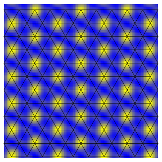
Figure 2: Charge density pattern at $1/3$-filling for $v>0$.

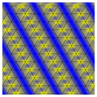
Figure 3: Charge density pattern at $1/3$-filling for $v<0$ and $w<0$.

Let us now proceed with the mean field theory for $f=1/3$. For $s<0$ and $|w|<|v|$ one obtains 3 distinct insulating phases:

I. $\boldsymbol{v>0}$:
The energy is minimized if only one of the 3 vortex flavors condenses. This state is then clearly 3-fold degenerate and breaks all symmetries except reflection with respect to $d_{2}$ axis. In Fig.2 this state is visualized explicitly by plotting the corresponding density wave order parameter. This state is the simplest CDW state at $1/3$-filling, with an example wavefunction consisting of a boson number eigenstate on each site. Microscopically this phase is the natural Mott insulating state in a model in which the Mott transition is driven by strong nearest-neighbor repulsive interactions, like the XXZ model. We do not expect the superfluid-Mott transition to this state is likely to be continuous or deconfined when fluctuations are taken into account in $2+1$ dimensions.

II. $\boldsymbol{v<0}$:
It is energetically favorable to condense all 3 vortex flavors, so that all vortex fields have equal magnitude. There are then 2 different phases, depending on the sign of $w$. These states are those expected to be connected by a deconfined quantum critical point to the superfluid state.

1. $w<0$.
   Writing $\xi_{\ell}\sim|\xi|e^{i\theta_{\ell}}$, the minimum is achieved when:

   $$\theta_{1}-\theta_{0}=2\pi m/3,\theta_{2}-\theta_{0}=2\pi n/3,$$ (45)

   for $m,n=0,1,2$.

   

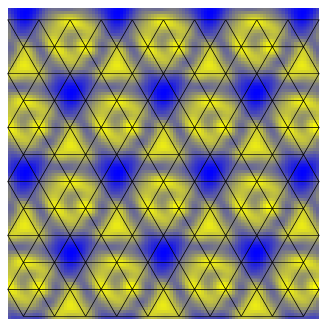
   Figure 4: Charge density pattern at $1/3$-filling for $v<0$ and $w>0$.

   This state is thus 9-fold degenerate and corresponds to period-3 site-centered stripes, running in ${\bf a}_{1},{\bf a}_{2}$ and ${\bf a}_{1}+{\bf a}_{2}$ directions, see Fig.3. One may construct a wavefunction for this state by e.g. taking linear 3-site clusters at a $60^{\circ}$ angle to the stripe (e.g. horizontal in Fig. 3), and putting a boson at the center of the cluster, leaving the other sites empty.

2. $w>0$.
   One can readily verify that the ground state is 18-fold degenerate, the distinct solutions being obtained from

   $$\theta_{1}-\theta_{0}=\theta_{2}-\theta_{0}=2\pi/9,$$ (46)

   by applying translations and the reflection $I_{d_{2}}$. The corresponding characteristic density pattern is shown in Fig.4. It is adiabatically connected to a “bubble” phase or crystalline state in which one boson is placed on each site of each elementary triangle (3 bosons total) on a $3\times 3$ triangular superlattice. The 18-fold degeneracy results from 9 states obtained by translating this pattern, and another 9 states obtained by choosing say down-pointing instead of up-pointing triangles.

III.3 $f=1/2$

III.3.1 Action and symmetries

We now turn to the more complicated and interesting case of $f=1/2$. It is straightforward to show (by a simple generalization of the argument used in Ref. Balents04, to prove the absence of a permutative representation in the $f=1/3$ case on the square lattice), that for this case there is no permutative representation of the PSG. Unlike in the square lattice case, there are also, surprisingly, more low-energy vortex modes for $f=1/2$ case than for $f=1/3$. The emergent low-energy symmetry amongst these modes is, moreover, nonabelian, with an $SU(2)$ “pseudo-spin” subgroup that we will uncover below. This structure has interesting consequences for the phases and excitations that will be explored here and in the following section in some detail.

The quartic potential can be found by solving Eq.(A). It turns out to have the following form:

$${\cal L}_{1}=u(\varphi^{*}_{\alpha\sigma}\varphi^{\vphantom{*}}_{\alpha\sigma})^{2}+v(\varphi^{*}_{+\sigma}\varphi^{\vphantom{*}}_{+\sigma})(\varphi^{*}_{-\sigma^{\prime}}\varphi^{\vphantom{*}}_{-\sigma^{\prime}})$$ (47)

$$+w\left(|\varphi_{-0}|^{2}|\varphi_{+0}|^{2}+\varphi^{*}_{-1}\varphi^{*}_{+1}\varphi_{-0}\varphi_{+0}+(0\leftrightarrow 1)\right).$$

To make the symmetries of the Lagrangian more transparent, it is useful to rewrite it as follows. First we define $z_{\alpha\sigma}$ pseudospinor variables,

$$\varphi_{-\sigma} = -\epsilon_{\sigma\sigma^{\prime}}z_{-\sigma^{\prime}},$$

$$\varphi_{+\sigma} = z_{\sigma},$$ (48)

where $\epsilon_{\sigma\sigma^{\prime}}$ is the antisymmetric tensor with $\epsilon_{01}=-\epsilon_{10}=1$. The quartic action has $SU(2)$ symmetry under rotations of the $\sigma$ index of $z_{\alpha\sigma}$. This is made manifest by introducing the pseudospin vector

$$S^{a}_{\alpha}=z^{*}_{\alpha\sigma}\tau^{a}_{\sigma\sigma^{\prime}}z^{\vphantom{*}}_{\alpha\sigma^{\prime}},$$ (49)

where $\tau^{a},\,a=x,y,z$ are the Pauli matrices, and summation on the repeated $\sigma,\sigma^{\prime}$ indices is implied. The transformation properties of the ${\bf S}_{\pm}$ vectors are particularly simple, and given in Appendix B. In terms of these pseudospin variables the quartic potential becomes, after a trivial redefinition of $v$ and $w$ couplings:

$${\cal L}_{1}=u\left(S_{+}+S_{-}\right)^{2}+v\,S_{+}S_{-}+w_{1}\,{\bf S}_{+}\cdot{\bf S}_{-},$$ (50)

where $S_{\alpha}=|{\bf S}_{\alpha}|=\sqrt{z_{\alpha\sigma}^{*}z_{\alpha\sigma}^{\vphantom{*}}}$ (sum on $\sigma$ implied). It is now clear that the quartic potential has, in addition to the microscopic gauge $U(1)$ symmetry, an $SU(2)\times U(1)\times Z_{2}$ invariance. The $SU(2)$ symmetry is manifest in Eq.(50), the extra $U(1)$ symmetry is the “staggered” $U(1)$, already mentioned above, see Eq.(30), also manifest since $S^{a}_{\alpha}$ are independent of the staggered $U(1)$ phase. The $Z_{2}$ symmetry is the interchange ${\bf S}_{+}\leftrightarrow{\bf S}_{-}$ (particle-hole symmetry $C$ in fact requires this invariance up to a sign, though Eq. (50) is obtained without using $C$). The pseudospin variables are directly related to the $\varrho^{\alpha}_{mn}$ density components:

$$\varrho^{\alpha}_{00}=S_{\alpha},$$

$$\varrho^{\alpha}_{01}=\alpha e^{\pi i(1+\alpha)/6}S_{\alpha}^{x},$$

$$\varrho^{\alpha}_{10}=\alpha e^{-\pi i(1+\alpha)/6}S_{\alpha}^{z},$$

$$\varrho^{\alpha}_{11}=S_{\alpha}^{y}.$$ (51)

The physical import of the $SU(2)$ symmetry of Eq. (50) is now clear: all CDW states, related to each other by arbitrary rotations in the space of the three Fourier components of the density, are degenerate at this order. This degeneracy will be weakly broken, of course, by higher order terms in the action. As discussed in the introduction, the large emergent symmetry is thereby connected with geometrical charge frustration at $f=1/2$.

III.3.2 Order parameters

The pseudospin vectors ${\bf S}_{\pm}$ serve as gauge-invariant order parameters to characterize the breaking of the $SU(2)$ symmetry. It is instructive to construct two other such order parameters. The emergent $U(1)$ symmetry is best characterized by a complex order parameter, $\psi$, defined by

$$\psi=e^{i\pi/4}z_{+\sigma}^{*}z_{-\sigma}^{\vphantom{*}},$$ (52)

where we have included the $\pi/4$ phase factor for later convenience. One may also define an Ising order paramer $\Phi$, with

$$\Phi=|z_{+}|^{2}-|z_{-}|^{2}.$$ (53)

Non-zero $\langle\Phi\rangle$ implies $I_{d_{2}}$ and $C$ are broken. The physical meaning of non-vanishing ${\bf S}_{\pm}$ and $\psi$ will be elucidated in detail in the following.

Though the terms which break these symmetries are small near the Mott QCP (hopefully irrelevant there), they are important at sufficiently low energy. We must therefore consider those higher order terms in the action which are required to reduce the $SU(2)\times U(1)$ symmetry to only what is required by the PSG. Higher order terms which do not reduce this symmetry need not be considered.

First consider the $SU(2)$ pseudospin symmetry. In the absence of microscopic particle-hole invariance, it is broken at $6^{\rm th}$ order by a term of the form $S_{+}^{x}S_{+}^{y}S_{+}^{z}+S_{-}^{x}S_{-}^{y}S_{-}^{z}$. We will, however, for concreteness focus on the case relevant to the XXZ model and other pairwise interacting boson lattice models, in which particle-hole symmetry is an invariance of the theory. In this case, the $SU(2)$ symmetry is broken only at the 8th order by a “cubic anisotropy” term,

$${\cal L}_{2}=w_{2}\sum_{\alpha}\left[\left(S^{x}_{\alpha}\right)^{4}+\left(S^{y}_{\alpha}\right)^{4}+\left(S^{z}_{\alpha}\right)^{4}\right].$$ (54)

The “staggered” $U(1)$ symmetry is more persistent and is broken at the 12th order. The simplest term at this order that breaks the “staggered” $U(1)$ symmetry is:

$${\cal L}_{3}=-w_{3}\,{\rm Re}\left(\psi^{6}\right).$$ (55)

Figure 5: Ordering wavevectors in the reciprocal lattice. Filled symbols are the wavevectors referred to in the text. Open symbols indicate wavevectors belonging to the same star which are related to the former sets by complex conjugation.

It is useful to reorganize various terms in the density expansion of Eq. (35) to understand in more detail the nature of the different order parameters. The wavevectors referred to in the following are labelled in Fig. 5.

Consider first Ising order. Non-zero $\langle\Phi\rangle$ implies only that the reflection $I_{d_{2}}$ and particle-hole symmetry $C$ are broken. Thus it corresponds only to a modulation of the density within the primitive unit cell of the triangular lattice. The corresponding density modulation therefore occurs entirely at reciprocal lattice vectors. The smallest set of reciprocal lattice wavevectors that can describe the modulation are ${\bf B}_{0}=(0,2\pi)$, ${\bf B}_{0}=(2\pi,-2\pi)$, ${\bf B}_{2}=(-2\pi,0)$. This density modulation is

$$\rho_{\Phi}({\bf r})=\Phi\sum_{n=0,1,2}\cos({\bf B}_{n}\cdot{\bf r}+\frac{5\pi}{6}).$$ (56)

While $\rho_{\Phi}=0$ on triangular (direct) lattice sites (as it must), it alternates sign on sites of the dual honeycomb lattice, i.e. takes opposite signs on centers of triangles of the direct lattice.

Now let us turn to pseudospin ordering. The existence of non-vanishing $\langle{\bf S}_{\pm}\rangle$ implies charge ordering at the wavevectors ${\bf G}_{x}=(0,-\pi)$, ${\bf G}_{y}=(-\pi,\pi)$, ${\bf G}_{z}=(\pi,0)$, which lie at the centers of the zone edges. In particular, the associated density modulations take the form

$$\rho_{S}({\bf r})=\sum_{a=x,y,z}{\rm Re}\,\left[(S_{+}^{a}e^{-i\pi/3}-S_{-}^{a})e^{i{\bf G}_{a}\cdot{\bf r}}\right],$$ (57)

neglecting higher harmonics which do not change the symmetry of $\rho_{S}({\bf r})$.

Next consider the XY order parameter $\psi$. A state with $\langle\psi\rangle$ exhibits a three-sublattice structure, characterized by the zone boundary wavevectors ${\bf Q}_{0}=2\pi(\frac{2}{3},-\frac{1}{3})$, ${\bf Q}_{1}=2\pi(-\frac{1}{3},\frac{2}{3})$, ${\bf Q}_{2}=2\pi(-\frac{1}{3},-\frac{1}{3})$:

$$\rho_{\psi}({\bf r})={\rm Re}\,\left[\psi e^{-i\pi/6}\sum_{n=0,1,2}\,e^{i2\pi n/3}e^{i{\bf Q}_{n}\cdot{\bf r}}\right].$$ (58)

In fact, these three wavevectors differ only by reciprocal lattice vectors. From this, it is straightforward to show that $\rho_{\psi}({\bf r})$ vanishes on dual lattice sites, so that all triangular plaquettes of the direct lattice are equivalent up to rotations in an XY ordered state.

Finally, simultaneous breaking of pseudospin and XY symmetry is characterized by the “composite” order parameter ${\bf d}$, a complex vector, defined as

$${\bf d}=z_{+\sigma}^{*}{\boldsymbol{\tau}}_{\sigma\sigma^{\prime}}z_{-\sigma^{\prime}}^{\vphantom{*}}.$$ (59)

When $\langle{\bf d}\rangle\neq 0$, density modulations appear at the wavevectors ${\bf K}_{x}=2\pi(\frac{1}{3},-\frac{1}{6})$, ${\bf K}_{y}=2\pi(-\frac{1}{6},-\frac{1}{6})$, ${\bf K}_{z}=2\pi(-\frac{1}{6},\frac{1}{3})$, which lie within the zone. The corresponding density is

$$\rho_{d}({\bf r})={\rm Re}\,\left[e^{3\pi i/4}\sum_{a=0,1,2}d_{a}e^{2\pi(a-1)i/3}e^{i{\bf K}_{a}\cdot{\bf r}}\right],$$ (60)

where we have identified $a=x,y,z$ with $a=0,1,2$ respectively.

III.3.3 Mean field phases

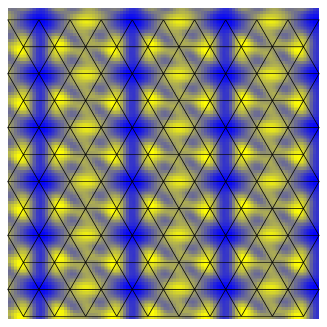
Figure 6: Charge density pattern at $1/2$-filling for $v<0$, $w_{1}<0$, $w_{2}<0$ and $w_{3}<0$.

The mean field phase diagram of ${\cal L}_{0}+{\cal L}_{1}+{\cal L}_{2}+{\cal L}_{3}$ can be easily obtained analytically. One finds 10 different phases: 2 for $v>0$ and 8 for $v<0$. We will not attempt to be exhaustive in describing these states. We will, however, discuss some of the phases in detail, and go into some general aspects of the 8 cases with $v<0$ in Sec. IV. Minimizing the mean-field energy functional, $v<0$ implies that both $\alpha=\pm$ vortex pseudospinors are condensed with equal amplitude, so $S_{+}=S_{-}$. The sign of $w_{1}$ determines the relative pseudospin orientation. For $w_{1}<0$, they are parallel, i.e. ${\bf S}_{+}={\bf S}_{-}\equiv{\bf S}$. In terms of the vortex variables this condition is most generally solved by

$$z_{\pm\sigma}=z_{\sigma}e^{\pm i\theta/2},$$ (61)

where ${\bf S}=z_{\sigma}^{*}{\boldsymbol{\tau}}_{\sigma\sigma^{\prime}}z_{\sigma^{\prime}}^{\vphantom{*}}$. For $w_{1}>0$, the two pseudospin vectors are antiparallel, ${\bf S}_{+}=-{\bf S}_{-}\equiv{\bf S}$, which implies

$$z_{+\sigma} = z_{\sigma}e^{i\theta/2},$$

$$z_{-\sigma} = \epsilon^{\vphantom{*}}_{\sigma\sigma^{\prime}}z^{*}_{\sigma^{\prime}}e^{i\theta/2}.$$ (62)

We note that the dual gauge symmetry acts differently in the two cases. For parallel pseudospins, a gauge transformation takes $z_{\sigma}\rightarrow e^{i\chi}z_{\sigma}$, while for antiparallel pseudospins, instead $\theta\rightarrow\theta+2\chi$.

The remaining terms, $w_{2}$ and $w_{3}$, fix the remaining non-gauge symmetries. The sign of $w_{2}$ chooses the easy axes of the pseudospin vector, along $(100)$ and symmetry-related axes for $w_{2}<0$, and along $(111)$ and related axes for $w_{2}>0$. The above conditions leave only the relative phase between the spinors $z_{\pm}$, corresponding to the “staggered” $U(1)$ symmetry of the corresponding terms in the vortex Lagrangian.

This relative phase is fixed at $12^{\rm th}$ order in $z_{\pm\sigma}$, for instance for $w_{1}<0$ by the ${\cal L}_{3}$ term (for $w_{1}>0$, a more complicated $12^{\rm th}$ order term must be included as the $w_{3}$ interaction vanishes in that case). Depending on the sign of $w_{3}$, the energy minimum is achieved when $\sin(6\theta)=\pm 1$, i.e.

$$\theta=\frac{\pi}{12}+\frac{\pi n}{3},\,\,n=0,\ldots,5,$$ (63)

or

$$\theta=\frac{\pi}{4}+\frac{\pi n}{3},\,\,n=0,\ldots,5,$$ (64)

One of the states, corresponding to $\theta=\pi/12$ and

$$z_{+0} = z_{+1}=\frac{e^{i\theta/2}}{\sqrt{2}},$$

$$z_{-0} = z_{-1}=\frac{e^{-i\theta/2}}{\sqrt{2}},$$ (65)

is shown in Fig.6. We will elucidate the physics of this particular pair of states in some detail in the discussion section.

We can generally classify all the mean field states by their degeneracies and the corresponding unit cell sizes. The states with the pseudospin easy axis along (100) and parallel pseudospins (the state in Fig.6 belongs to this group) are all 36-fold degenerate and have a 6-site unit cell. States with parallel pseudospins but with the easy axis along (111) are 48-fold degenerate and have the largest, 12-site unit cell. In the case of antiparallel pseudospins, ground state degeneracies are the same, but the unit cell size of the 36-fold degenerate states doubles to 12 sites. States with the smallest unit cells are obtained when only one of the pseudospinors is condensed. In this case one obtains a 6-fold degenerate ground state and a 2-site unit cell when (100) is the easy axis, and an 8-fold degenerate state with a 4-site unit cell when the easy axis is along the (111) direction.

For the phases of most interest ($v<0$) in which the pseudospin vectors are either parallel or antiparallel, some of the density functions associated to the order parameters in Sec. III.3.2 can be simplified to an extent. The only qualitative case is the pseudospin vector density $\rho_{S}$. When ${\bf S}_{+}={\bf S}_{-}={\bf S}$, it reduces to

$$\rho_{S\parallel}({\bf r})=\sum_{a=x,y,z}S^{a}\cos({\bf G}_{a}\cdot{\bf r}-\frac{2\pi}{3}).$$ (66)

Most interesting, when ${\bf S}_{+}=-{\bf S}_{-}={\bf S}$, one has instead

$$\rho_{S,\not\parallel}({\bf r})=\sum_{a=x,y,z}S^{a}\cos({\bf G}_{a}\cdot{\bf r}-\frac{\pi}{6}).$$ (67)

In this case, it is noteworthy that $\rho_{S,\not\parallel}$ vanishes on all triangular lattice sites. This is a consequence of the fact that a configuration of antiparallel pseudospins preserves particle-hole symmetry, so modulations can occur only in bond or plaquette “kinetic” terms. Thus ${\bf S}_{+}-{\bf S}_{-}$ may be considered a (particular) purely valence bond solid order parameter.

The composite order parameter ${\bf d}$ also simplifies once the pseudospin order is determined. For parallel pseudospins, one simply has ${\bf d}={\bf S}$. For antiparallel pseudospins, instead, one has ${\bf d}\times{\bf d}^{*}=2i{\bf S}$, which implies

$${\bf d}={\bf e}_{1}-i{\bf e}_{2},\qquad{\bf e}_{1}\times{\bf e}_{2}={\bf S},$$ (68)

so that ${\bf e}_{1},{\bf e}_{2},{\bf S}$ form a right-handed orthogonal frame in the O(3) spin space. The angle of ${\bf e}_{1}$ in the XY plane is arbitrary, and determined by (twice) the phase of $z_{\sigma}$.

IV “Hard Spin” Description: Beyond Mean-Field Theory

In the preceding section, we have followed a Landau-theory like procedure (albeit with non-LGW vortex fields) in expanding the effective action in a power series in the $\varphi_{\ell}$ fields, whose amplitude is viewed as small in the vicinity of the Mott QCP. In low-dimensional statistical mechanics, it is often preferable to formulate the theory in terms of “hard spin” variables, in which the amplitude of the order parameter field(s) is fixed, and only the “angular” degrees of freedom are free to fluctuate and vary in space and time. Examples include the Kosterlitz-Thouless theory of the XY phase transition, and the non-linear sigma model formulation of $O(n)$ models. The intuitive rationale for such an approach is that, in low dimensions, fluctuations suppress the ordering point of the transition well below the mean-field point, so that substantial amplitude is already developed in the true critical region. Whatever the rationale, there are some advantages to such a hard-spin approach. Duality transformations generally apply to hard-spin models. Hard-spin variables are particularly appropriate to describe the elementary excitations of “ordered” phases in which the amplitude of the fields is on average large, and only the Goldstone-like fluctuations of the orientation of these fields comprise low-energy excitations. Finally, a hard-spin formulation returned to the lattice is fully-regularized, and can thereby address non-perturbative phenomena in a controlled manner.

In this section, we will provide and analyze a hard-spin formulation of the dual vortex action. These allow us to identify the excitations and their quantum numbers within the Mott phases. Notably, we find that the most interesting Mott states support two distinct kinds of excitations. First, there are $1/2$-charged (“spinon” in the spin-$1/2$ XXZ language) “vortex” excitations which are linearly confined in pairs deep in the Mott state, but are only logarithmically interacting up to a long “confinement length” near the superfluid-Mott transition. Second, there are additional unit charged “skyrmion” excitations which are everywhere deconfined in the Mott state. These are adiabatically connected to single boson vacancies/interstitials in the Mott solid, but become topological as the Mott transition is approached. The hard-spin models also provide a firm ground on which to study other phases, notably supersolids, which do not occur within a mean field treatment of the vortex field theory, but are extremely natural in this approach.

IV.1 Formulation of hard spin model

To write down an appropriate hard-spin model, we imagine tuning $s<0$ to a point beyond the mean field Mott transition point. At such a point, the minimum action configurations have non-zero amplitude. We will assume the mean amplitude is determined by a balance between the quadratic Lagrangian, Eq. (25) and the quartic terms in ${\cal L}_{1}$, Eq. (50). The minimum action saddle points of the combination of these two terms are constant in space-time, but allow for a continuous set of orientations in the field space. We focus in particular on $v<0$, so that the magnitude $S_{+}=S_{-}$ is fixed. We will focus primarily on the case $w_{1}<0$, so that the saddle point has ${\bf S}_{+}={\bf S}_{-}$. This is the most interesting case, because, as we shall see, the recently-determined supersolid phase of the XXZ model can be understood in this framework. At the end of this section, we will briefly summarize the results of similar analysis for $w_{1}>0$, corresponding to anti-parallel pseudospins.

We further suppose that $s$ is negative enough that fluctuations in the above conditions may be neglected, but that within these constraints the $z_{\alpha\sigma}$ fields can vary spatially. We will therefore absorb any effects of the magnitude of the fields into coefficients, and without loss of generality normalize to $S_{+}=S_{-}=1$. Ultimately, the higher order terms will still be included, but can be considered small perturbations.

The most general solution of ${\bf S}_{+}={\bf S}_{-}={\bf S}$ constraint in terms of the vortex variables is given by Eq. (61). We will therefore rewrite the action in terms of the CP¹ field $z_{\sigma}$ and an XY field $e^{i\theta/2}$. Note that this solution possesses a $Z_{2}$ gauge invariance under

$$z_{\sigma}\rightarrow-z_{\sigma},\qquad\theta\rightarrow\theta+2\pi.$$ (69)

This is in addition to the physical symmetries of the model. It is a gauge invariance since it can be performed independently at each space-time point without changing $z_{\alpha\sigma}$, and hence physical quantities.

Inserting Eq. (61) into the action, and regularizing it on a space-time lattice, we obtain

$${\cal L}_{\rm HS}^{\parallel}=-t_{v}e^{-iA_{i\mu}}z^{*}_{i\sigma}z_{i+\mu\sigma}\cos(\Delta_{\mu}\theta_{i}/2)+\frac{1}{2e^{2}}(\epsilon_{\mu\nu\lambda}\Delta_{\nu}A_{i\lambda})^{2},$$ (70)

with $z_{i\sigma}^{*}z_{i\sigma}^{\vphantom{*}}=1$ normalized on each site $i$ of the space-time lattice. Note that Eq. (70) is indeed invariant independently under Eq. (69) at each point $i$. It is convenient to rewrite the first term in Eq. (70), making the Ising gauge symmetry explicit by introducing an Ising gauge field $\sigma_{i\mu}$ which resides on the link $(i,i+\mu)$:

$${\cal L}_{\rm Z_{2}}^{\parallel} = -t_{z}\sigma_{i\mu}e^{-iA_{i\mu}}z^{*}_{i\sigma}z_{i+\mu\sigma}-t_{\theta}\sigma_{i\mu}\cos(\Delta_{\mu}\theta_{i}/2)$$ (71)

$$+\frac{1}{2e^{2}}(\epsilon_{\mu\nu\lambda}\Delta_{\nu}A_{i\lambda})^{2},$$

where we have introduced two independent parameters $t_{z},t_{\theta}$. One could add a plaquette interaction (line product of $\sigma_{i\mu}$ around plaquettes), which is a standard “kinetic term” for the $Z_{2}$ gauge field for further generality. We are, however, most interested in the limit in which it is absent. In this case, one may sum over $\sigma_{i\mu}$ on each link independently, to return to an action of the form of Eq. (70) (with additional higher-order terms). We will not attempt, however, to constrain Eq. (71) to be exactly equivalent to Eq. (70). Instead, since we are anyway constructing a phenomenological theory, we regard the freedom to vary $t_{z},t_{\theta}$ independently as a means of capturing the different possible tendencies due to fluctuation effects and details of microscopic dynamics in different physical systems.

IV.2 Phase diagram for parallel pseudospins

Let us now discuss the phase diagram of Eq. (71). For $t_{z},t_{\theta}\ll 1$, both $\theta_{i}$ and $z_{i\sigma}$ variables are disordered, and the dual gauge field $A_{i\mu}$ is gapless. This is the superfluid phase. For $t_{\theta}\sim t_{z}\gg 1$ large and of the same order, we expect that both the CP¹ and XY variables are ordered. This is the Mott insulator, whose precise nature depends upon the anisotropy terms we have neglected to write.

Now suppose $t_{\theta}\gg 1$ but $t_{z}\ll 1$. In this limit, we expect the XY variables condense. This is a “Higgs” phaseKogut from the point of view of the $Z_{2}$ gauge variables: the linear coupling to $\cos(\Delta_{\mu}\theta_{i}/2)$ means that the $\sigma_{i\mu}$ fields can be regarded as having some non-vanishing expectation value in this state. The CP¹ fields however remain uncondensed, and $A_{i\mu}$ remains gapless, so this state retains superfluidity. It does, however, break spatial symmetry. To understand the nature of this symmetry breaking, let us take for simplicity $t_{z}=0$, and again imagine “summing out” the $Z_{2}$ gauge fields while varying $t_{\theta}$. The effective Lagrange density is then

$${\cal L}_{XY} = V(\Delta_{\mu}\theta_{i})+\frac{1}{2e^{2}}(\epsilon_{\mu\nu\lambda}\Delta_{\nu}A_{i\lambda})^{2}$$ (72)

with $V(\Theta)=-\ln\cosh\left[\frac{t_{\theta}}{\sqrt{2}}\sqrt{1+\cos(\Theta)}\right]$. This somewhat unconventional gradient term has all the same symmetries as the usual $\cos(\Delta_{\mu}\theta_{i})$ term in an XY model, and indeed reduces to that form for small $t_{\theta}$. On increasing $t_{\theta}$, therefore, a 3D=2+1 dimensional XY transition is expected, into a state with a non-zero expectation value of $e^{i\theta}$. Comparison with Eq. (52) indicates that $\psi\sim e^{i\pi/4}e^{-i\theta}$ is an order parameter for this transition. Note that $e^{i\theta_{i}/2}$ is not an order parameter since it is not ($Z_{2}$) gauge invariant. As noted earlier, $\psi$ is exactly the order parameter identified in Refs. Melko05, ; Damle05, ; Troyer05, as characterizing the supersolid phase of the XXZ model on the triangular lattice. This supersolid has a three-sublattice structure, so we will denote it by SS3. Actually there are two different ordering patterns possible within the tripled unit cell, depending upon the sign of the $6$-fold anisotropy term, $w_{3}$, which should be added to Eq. (72). They are shown in Fig. 7.

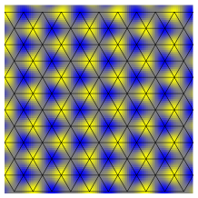
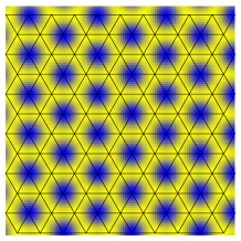
Figure 7: Possible charge ordering patterns in the SS3 phases. Left: “antiferromagnetic” supersolid ($w_{3}>0$). Right: “ferrimagnetic” supersolid ($w_{3}<0$).

Finally, consider similarly the situation when $t_{\theta}\ll 1$ but $t_{z}$ varies from small to large. For large $t_{z}$, we then expect the CP¹ variables order but the XY variables remain uncondensed. Analogously to the previous case, imagine increasing $t_{z}$ from small to large with $t_{\theta}=0$. One can again integrate out the Ising gauge field to obtain an effective action which is $Z_{2}$-gauge invariant. In this case, there are two distinct types of “kinetic” terms which arise on nearest-neighbor bonds. For small $t_{z}$, they take the form

$${\cal L}_{SU(2)} = -t_{S}{\bf S}_{i}\cdot{\bf S}_{j}-t_{2}e^{-2iA_{i\mu}}z_{i\sigma}^{*}z_{i\sigma^{\prime}}^{*}z_{i+\mu,\sigma}^{\vphantom{*}}z_{i+\mu,\sigma^{\prime}}^{\vphantom{*}}$$ (73)

$$+\frac{1}{2e^{2}}(\epsilon_{\mu\nu\lambda}\Delta_{\nu}A_{i\lambda})^{2},$$

where $t_{S},t_{2}\sim t_{z}^{2}$ and ${\bf S}_{i}=z_{i}^{*}{\boldsymbol{\tau}}z_{i}^{\vphantom{*}}$. Two distinct types of “orderings” are clearly possible on increasing $t_{z}$. The most natural possibility, driven by $t_{S}$, is for ${\bf S}$ to order. As above, this is a supersolid, but with a different set of possible charge order patterns, characterized by the zone boundary center wavevectors rather than those at zone corners. An alternative possibility, driven by $t_{2}$, is that the vortex pair field $z_{i\sigma}z_{i\sigma^{\prime}}$ condenses. Such a paired vortex condensate is a spin-liquid insulator (see Ref. Balents00, ) (a “$Z_{2}$” spin liquid in the now-conventional nomenclatureSenthilFisher ; Wen91 ). The $A_{i\mu}$ gauge fluctuations will tend to suppress such pair field condensation, so we expect the supersolid phase with $\langle{\bf S}\rangle\neq 0$ to occur first on increasing $t_{z}$. Such supersolid states have a maximum period of $2$ lattice sites along the principle axes of the triangular lattice (as can be seen from the behavior of translations in Eqs. (142), so we denote these phases by SS2 (they may have doubled or quadrupled unit cells, depending upon the orientation of the pseudospin vector). The two different ordering patterns for different signs of $w_{2}$ are shown in Fig. 8.

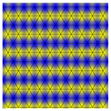
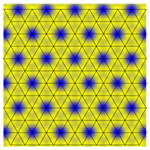
Figure 8: Possible charge orderings in the SS2 phases. Left: ${\bf S}=(100)$. Right: ${\bf S}=(111)$.

Putting the different limits of this analysis together and making the simplest possible interpolation, we expect the phase diagram in Fig. 9. The Mott state may be reached from the superfluid in at least three distinct ways: by a direct transition described by the continuum vortex Lagrangian in the previous section, or via two distinct intermediate supersolid phases. The transitions from the superfluid to the two supersolids are “conventional”, i.e. of LGW type, since they are described by ordering of the gauge-invariant order parameters $\psi$ and ${\bf S}$. The transitions from the supersolids, by contrast, are unconventional. This is clear from the fact that the Mott insulator differs from either supersolid by breaking more spatial symmetry and by having no off-diagonal long range order, i.e. by being non-superfluid. Thus two symmetry-unrelated order parameters must change in these transitions. We will return to the nature of these transitions after first discussing the elementary excitations of the different phases.

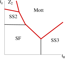
Figure 9: Schematic phase diagram of the $Z_{2}$ hard spin model. Thin lines denote conventional LGW-type transitions, thick (red online) lines denote non-LGW quantum critical points.

IV.3 Elementary excitations

IV.3.1 Superfluid phase

The hard spin model is convenient for describing the elementary excitations of the phases discussed above. First consider the superfluid. In this case, the elementary excitations are simply vortices, and the vortex field theory of the previous two sections already gives a description of the elementary vortex multiplet, consisting in this case of $4$ vortex flavors (carrying pseudospin-$1/2$ and XY “charge” $\pm 1/2$). This should be reproduced by the hard spin model. Naïvely, the “particles” of the hard spin model are created separately by the $z_{\sigma}$ and $e^{\pm i\theta/2}$ fields, so carry only one or the other of pseudospin or XY charge. However, in the superfluid region of Fig. 9, the $Z_{2}$ gauge charges (whose interactions are mediated by $\sigma_{i\mu}$) are confined, so the true elementary excitations are $Z_{2}$ gauge-neutral bound states $\sim e^{\pm i\theta/2}z_{\sigma}$ which have precisely the appropriate quantum numbers of the $z_{\pm\sigma}$ vortices.

IV.3.2 Mott phase

Next consider the Mott state. In reality this comprises a number of different phases, depending upon the signs of the anisotropies $w_{2},w_{3}$. However, near to the superfluid-Mott transition, the latter terms are small, and these distinct phases are approximately unified into one continuous manifold. It is useful to discuss the elementary excitations therefore in the same approximation, and afterward describe how they are modified once anisotropy is included. From the point of view of the $Z_{2}$ hard spin model, Eq. (71), the Mott state is a Higgs phase, with both XY and CP¹ fields condensed. The $Z_{2}$ gauge field can be regarded, in a choice of gauge, as uniform $\sigma_{i\mu}\approx 1$, in the ground state. If we neglect the possibility of deforming the $Z_{2}$ gauge field in excited states, there are then two “obvious” topological excitations – time independent solitons that behave as quantum particles – corresponding to textures in the CP¹ and XY fields.

First consider the CP¹ field. At spatial infinity, $z_{i\sigma}$ must vary slowly in space to maintain minimal action, as must $A_{i\mu}$ for the same reason. We may therefore take a continuum limit of the first term in Eq. (71), and, taking $\sigma_{i\mu}\rightarrow 1$, one finds the Lagrangian

$${\cal L}_{z} \approx \frac{1}{2}\varrho_{s}|\partial_{\mu}{\bf S}|^{2}+\kappa({\cal C}_{\mu}-A_{\mu})^{2}$$ (74)

$$+\frac{1}{2e^{2}}(\epsilon_{\mu\nu\lambda}\partial_{\nu}A_{i\lambda})^{2}$$

with $\varrho_{s},\kappa\sim t_{z}$, and

$${\cal C}_{\mu}=-\frac{i}{2}\left(z^{*}_{\sigma}\partial_{\mu}z^{\vphantom{*}}_{\sigma}-\partial_{\mu}z^{*}_{\sigma}z^{\vphantom{*}}_{\sigma}\right).$$ (75)

Minimum action configurations therefore have $\partial_{\mu}{\bf S}=0$ and $A_{\mu}={\cal C}_{\mu}$ at infinity. This requires that, at infinity, only the phase of the spinor varies, i.e. $z_{\sigma}=\xi_{\sigma}e^{i\Theta}$, where $\xi_{\sigma}$ is a constant normalized spinor, and $\Theta$ may depend upon the polar angle from the origin. At infinity, then

$${\cal C}_{\mu}=\partial_{\mu}\Theta.$$ (76)

Single-valuedness of $z_{\sigma}$ allows topologically non-trivial configurations in which $\Theta$ winds by an integer multiple of $2\pi$, whence

$$\oint dx_{\mu}{\cal C}_{\mu}=\oint dx_{\mu}A_{\mu}=2\pi n_{s},$$ (77)

the integer $n_{s}$ being a topological index. Thus the dual flux of such configurations is quantized in units of the dual flux quantum. Since the dual flux measures physical charge, such solitons are particle-like excitations of the Mott state with physical integral boson charge $n_{s}$. While at infinity the spinor varies only through $\Theta$, (and hence the pseudospin ${\bf S}$ is constant), this cannot hold everywhere in space, since such a “vortex” in $\Theta$ must have a singularity somewhere. If the spinor is assumed to vary everywhere slowly in space, so that a uniform continuum limit can be taken everywhere, then the singularity is avoided by having the associated amplitude vanish at the skyrmion’s “core”, e.g. in a configuration of the form

$$z_{\sigma}=f(r)e^{i\Theta}\xi_{\sigma}+\sqrt{1-f(r)}\eta_{\sigma},$$ (78)

where $\xi_{\sigma}$ and $\eta_{\sigma}$ are two normalized orthogonal constant spinors, $\xi_{\sigma}^{*}\eta_{\sigma}^{\vphantom{*}}=0$, and $f(r)\rightarrow 1$ as $r\rightarrow\infty$, $f(r)\rightarrow 0$ as $r\rightarrow 0$ ($r$ is the radial coordinate from the skyrmion center). The non-collinear variation of $z_{\sigma}$ indicates a non-trivial texture of the pseudospin in the skyrmion. Quite generally, if $z_{\sigma}$ is analytic, one can show that

$$n_{s}=\frac{1}{4\pi}\int d^{2}r\,{\bf S}\cdot\partial_{x}{\bf S}\times\partial_{y}{\bf S},$$ (79)

directly relating the skyrmion number to the pseudospin texture. Because the pseudospin itself is constant at infinity, it is apparent that the skyrmion has a finite size, in the example of Eq. (78) determined by the range of significant spatial variation of $f(r)$. This scale is dependent upon details of the Hamiltonian within the Mott phase, and in general the above description of the spatially-varying pseudospin is valid only if this scale is much larger than the unit cell of the Mott charge ordering pattern. Deep in the Mott phase (i.e far from the Mott transition), this may not be the case, and in that case there is not necessarily any sharp meaning to the pseudospin texture. In this sense, the skyrmion/antiskyrmion can be considered as adiabatically connected to a simple, and patently non-topological, vacancy or interstitial defect of the Mott “solid”.

Near to the Mott transition, however, the skyrmion is expected to be large, as we now show. The size of the skyrmions is determined by the balance of the anisotropy energy ${\cal L}_{2}$ and the interaction energy $(\epsilon_{\mu\nu\lambda}\partial_{\nu}A_{\lambda})^{2}$. A rough estimate for the skyrmion size can be obtained by a simple dimensional analysis. The anisotropy energy of a skyrmion of size $\lambda$ is of the order of $w_{2}|S|^{4}\lambda^{2}$, where $|S|$ is the unrescaled amplitude of the pseudospin vector order parameter. On the other hand, the interaction energy is of the order $1/e^{2}\lambda^{2}$. The optimal skyrmion size is therefore given by:

$$\lambda\sim(w_{2}|S|^{4}e^{2})^{-1/4}.$$ (80)

Close enough to the critical point, since $|S|$ becomes small, the skyrmion becomes large, and thus develops a topological character.

Now consider the excitations of the XY field. Taking $\sigma_{i\mu}\approx 1$ in Eq. (71), the naïve topological excitation consists of winding $\theta$ at infinity by an integer multiple of $4\pi$ – not $2\pi$, since the $\cos(\Delta_{\mu}\theta_{i}/2)$ is not $2\pi$-periodic. These excitations are paired vortices in the 3-sublattice supersolid order parameter $\psi$. They are neutral, since there is no coupling to the dual gauge field. Like an ordinary neutral superfluid vortex, they cost a logarithmic energy, neglecting the XY anisotropy term $w_{3}$. When it is included, such a (double-strength) $\psi$ vortex becomes linearly confined, and converts at long distances to an intersection point of 12 (!) domain walls, the phase winding coalescing into these 12 walls radiating outward from the “vortex” core.

Allowing for a non-trivial texture in the $Z_{2}$ gauge field, however, a third kind of excitation is possible in the Mott phase. In particular, one may consider a “vison” or $Z_{2}$ vortex, around a point around which any line product of Ising gauge fields gives $-1$. This requires the existence of a “cut”, a ray emanating outward from the vison along which Ising gauge fields crossing the ray are taken negative (nevertheless, the $Z_{2}$ flux is non-trivial only through one plaquette at the vison core). Such a cut effectively introduces anti-periodic boundary conditions for both $z_{\sigma}$ and $e^{i\theta/2}$ across the cut. That such a configuration is possible is of course evident from the definition of $z_{\sigma}$ and $\theta$ in Eq. (61), since the apparent discontinuities in $z_{\sigma}$ and $e^{\pm i\theta/2}$ do not affect the elementary $z_{\pm\sigma}$ fields. The anti-periodic boundary condition forces topological defects into both the XY and CP¹ fields. In the XY sector, it requires the existence of a $\pm 2\pi$ vortex in $\psi$. As for the $\pm 4\pi$ vortex above, this costs logarithmic energy neglecting $w_{3}$, and degenerates into a linearly confined “source” for (in this case 6) radial domain walls. In the CP¹ sector, it is slightly less intuitive. One might have expected the occurrence of some sort of “half-skyrmion” pseudospin texture. However, this is not the case. Anti-periodic boundary conditions require the discontinuity to persist all the way down from infinity to the vison core. There is thus no way to “relax” the winding singularity at infinity into a smooth pseudospin texture. Instead, the minimal energy configuration has ${\bf S}$ spatially constant everywhere, i.e. has the form $z_{\sigma}=\xi_{\sigma}e^{i\Theta}$, where $\Theta$ winds by $\pm\pi$ and $\xi_{\sigma}$ is constant everywhere save in some small core region of microscopic size. However, the continuum action Eq. (74) still obtains at infinity, so that finite energy configurations still satisfy Eq. (76) and $A_{\mu}={\cal C}_{\mu}$ at infinity. Hence, these CP¹ “half-vortex” configurations carry fractional boson charges $\pm 1/2$. So by taking into account $Z_{2}$ gauge vortices, we find a third class of “elementary” excitations in the Mott insulator, “half bosons” with a texture in the 3-sublattice supersolid order parameter $\psi$. These are linearly confined beyond some length at which the 6-fold XY anisotropy becomes significant.

Of the three types of topological excitations discussed, it is interesting to note that only the charge $\pm 1$ skyrmion remains unconfined at the longest scales.

IV.3.3 SS3 phase

Let us now turn to the SS3 phase, which is described by Eq. (71) at large $t_{\theta}$. As discussed above, the ground state in this limit can be regarded as a $Z_{2}$ Higgs phase, with the $z_{\sigma}$ field uncondensed. Hence there are two types of topological defects: “paired” XY vortices in $\psi$, in which $\theta$ winds by a multiple of $4\pi$ and single XY vortices, in which $\psi$ winds by $\pm 2\pi$, accompanied by a vison. Both cost logarithmic energy at short scales, crossing over to linear confinement as do similar excitations in the Mott state. Finally, there are the CP¹ “particles” created by the $z_{\sigma}$ field, which can be considered to propagate coherently since the $Z_{2}$ gauge field is in a Higgs phase. The single XY vortices have a statistical interaction with the CP¹ quanta, but this does not lead to significant effects upon the CP¹ particles since the XY vortices are anyway linearly confined. The CP¹ quanta still carry unit dual gauge charge, and so should be regarded as the physical superfluid vortex excitations of the supersolid.

IV.3.4 SS2 Phase

The pseudospin vector order parameter ${\bf S}=z^{*}{\boldsymbol{\tau}}z^{\vphantom{*}}$ is condensed in the SS2 phase. However, it is not a Higgs phase for the $z_{\sigma}$ fields, since, for instance, it is still superfluid, i.e. the dual gauge field remains gapless. Thus in the SS2 phase $Z_{2}$ quanta are strongly confined, and the elementary excitations must be $Z_{2}$ singlets. One class of excitations are skyrmions in ${\bf S}$. They do not carry any well-defined charge since the boson number conservation symmetry is anyway broken in the supersolid. The other quanta are physical vortices, which are bound states of $z_{\sigma}$ and $e^{\pm i\theta/2}$ particles, essentially the original $z_{\pm\sigma}$ vortices of the superfluid. However, because of the broken pseudospin symmetry in this phase, there is a preferred pseudospin polarization, and the two $\sigma$ components of the vortex spinor (choosing a quantization axis along ${\bf S}$) are no longer energetically equivalent. Therefore there is only a two-fold rather than four-fold low-energy vortex multiplet $\xi_{\pm}\sim z_{\pm 0}$, taking $\sigma=0$ as the lower-energy spinor.

IV.4 Supersolid-Mott quantum critical points

IV.4.1 SS3-Mott transition

The supersolid to Mott insulator QCPs are manifestly not of LGW type, if they occur at all as continuous transitions. Nevertheless, at least some aspects of these QCPs can be straightforwardly analyzed by application of Eq. (71). Consider first the SS3-Mott transition. It is useful to approach the transition first from the SS3 phase. Since it can be regarded as a $Z_{2}$ Higgs state, this is particularly simple. In particular, we can treat $\sigma_{i\mu}\approx 1$ as a constant at low energies. The $e^{\pm i\theta_{i}/2}$ fields can be regarded as condensed, and moreover at low energies there are no associated gapless Goldstone modes due to the 6-fold anisotropy term $w_{3}$ in Eq. (55). Hence at low energies, the only important fluctuations are those of the CP¹ spinor and the dual gauge field. The natural critical theory, kept lattice regularized for simplicity, and neglecting for the moment pseudospin anisotropy, is thus just

$${\cal L}_{NCCP1} = -t\sigma_{i\mu}e^{iA_{i\mu}}z^{*}_{i\sigma}z_{i+\mu\sigma}+\frac{1}{2e^{2}}(\epsilon_{\mu\nu\lambda}\Delta_{\nu}A_{i\lambda})^{2}.$$

This is the Non-Compact CP¹ (NCCP¹) theory studied numerically in Ref. Lesik, , and believed to represent a distinct universality class of critical phenomena. It also has a more intuitive interpretation: it describes the behavior of the $2+1=3$ dimensional $O(3)$ transition associated with ${\bf S}$ when “hedgehog” defects in ${\bf S}$ are completely suppressed in the partition function. Let us now see how this is understood approaching the QCP from the Mott side. In this phase, the pseudospin vector is ordered, but fluctuates more and more strongly as the SS3 phase is approached. One would expect skyrmion defects to become more and more prevalent as fluctuations in the pseudospin increase. As described above in Sec. IV.3.2, however, skyrmions in the Mott state carry physical boson charge, so boson number conservation requires that skyrmion-number ($n_{s}$ in Eq. (79)) must also be conserved. Happily, skyrmion number-changing events are exactly the hedgehog defects of the $O(3)$ model, so we see that charge conservation causes this transition to be of the NCCP¹ type.

Eq. (IV.4.1) and the subsequent discussion neglect pseudospin anisotropy. While it is quite likely such anisotropy terms are irrelevant the NCCP¹ fixed point, this requires further study. Using the hard-spin PSG transformations, Eqs. (163), the leading anisotropy terms can be shown to be

$${\cal L}^{\prime}_{NCCP1} = w_{2}\!\!\!\!\sum_{a=x,y,z}\!\!(S^{a})^{4}+w^{\prime}_{2}\left({\rm Im}\,\psi^{3}\right)S^{x}S^{y}S^{z}.$$ (82)

The latter term is allowed by symmetry, but vanishes for $w_{3}>0$, in which case $\psi^{3}$ is purely real. Note that the perturbations $w_{2},w^{\prime}_{2}$ in Eq. (82) are $8^{\rm th}$ and $6^{\rm th}$ order in the CP¹ fields, respectively, so it is quite plausible that both are irrelevant at the NCCP¹ point, though clearly this is most likely for $w_{3}>0$, when the $w^{\prime}_{2}$ term is absent.

A further complication in the case $w_{3}<0$ is that the non-vanishing $\psi$ order parameter in this case breaks particle-hole symmetry $C$ (actually the supersolid with $w_{3}>0$ also breaks C, but preserves the combination $C\circ T_{2}\circ R_{2\pi/3}\circ I_{d_{1}}\circ I_{d_{2}}$, which is sufficient). Since a supersolid, like a superfluid, is compressible, this has the difficulty that it implies a non-vanishing deviation of the spatially averaged density from half-filling (working at fixed chemical potential chosen to maintain particle-hole symmetry – i.e. zero Zeeman field in the XXZ model). In the canonical ensemble, fixing the average density at $f=1/2$, it implies phase separation. Formally, this is described in the dual theory by the allowed coupling term

$${\cal L}^{\prime\prime}=\lambda\left({\rm Im}\,\psi^{3}\right)(\Delta_{x}A_{y}-\Delta_{y}A_{x}),$$ (83)

since the physical density is the dual magnetic flux. This indeed leads to a density deviation from half-filling away from the NCCP¹ critical point, since it leads to a minimum of ${\cal L}_{NCCP1}+{\cal L}^{\prime\prime}$ with non-zero $\delta n\sim(\Delta_{x}A_{y}-\Delta_{y}A_{x})/2\pi$. As the Mott transition is approached, however, the system becomes increasingly less compressible, and the compressibility certainly vanishes when superfluidity does. It is not entirely clear to us how this is resolved – the complications are similar to (but more difficult due to the pseudospin structure) those occuring in the theory of the normal-superconducting thermal phase transition in a three-dimensional superconductor in a weak applied external field $H$.NelsonSeung It is possible that, at fixed chemical potential, the NCCP¹ critical fixed point is “weakly avoided” at long scales by this effect, most likely by introducing a narrow region of an “SS6” phase – a supersolid with the same symmetry as the Mott insulator but with ODLRO – between the Mott insulator and ferrimagnetic SS3 state. Working at fixed density $f=1/2$, one expects to pass through the NCCP¹ point, which coincides with the critical endpoint of the phase separation region.

IV.4.2 SS2 to Mott transition

As indicated in Sec. IV.3.4, the SS2 phase should be thought of as a state in which $\langle{\bf S}\rangle\neq 0$, but vortices themselves are not condensed. It is not, however, a Higgs phase of Eq. (71). Moreover, the important elementary excitations of this phase are just vortices, which are bound states of the hard-spin fields. Therefore it is advantageous to return to the original soft-spin vortex formulation, and procede by just adding the term

$${\cal L}^{\prime}_{SS2}=-\lambda\langle{\bf S}\rangle\cdot({\bf S}_{+}+{\bf S}_{-}),$$ (84)

where of course the ${\bf S}_{\pm}$ fields on the right should be understood as composites of $z_{\pm\alpha}$. As discussed in Sec. IV.3.4, this splits the 4-fold vortex multiplet into two 2-fold multiplets. Taking $\langle{\bf S}\rangle$ along $(100)$ (we will not discuss the $(111)$ case in any detail, but it is similar), we obtain the scalar low energy fields $z_{\pm}$, defined by $z_{\pm\alpha}=z_{\pm}\eta_{\alpha}$, with $\tau^{x}\eta=+\eta$ (other orientations are solved by the obvious generalization). By considering the residual symmetry operations of this SS2 state (see Appendix D), we may thereby derive the continuum action for these two fields:

$${\cal L}=\sum_{\alpha=\pm}\left[|(\partial_{\mu}-iA_{\mu})z_{\alpha}|^{2}+s|z_{\alpha}|^{2}\right]+u(z_{\alpha}^{*}z_{\alpha}^{\vphantom{*}})^{2}$$ (85)

$$-v|z_{+}|^{2}|z_{-}|^{2}+\lambda\,{\rm Im}\,(z_{+}^{*}z_{-}^{\vphantom{*}})^{6}+\frac{1}{2e^{2}}(\epsilon_{\mu\nu\lambda}\partial_{\nu}A_{\lambda})^{2}.$$

Here we have kept the $12^{\rm th}$ order $\lambda$ term because it is the lowest order term which breaks the staggered $U(1)$ symmetry.

Remarkably, Eq. (85) is extremely similar to the NCCP¹ Lagrangian, differing mainly in that the SU(2) symmetry of that theory is here reduced by the $v$ term to U(1). For $v>0$, corresponding to the easy-plane case, it is the continuum theory for the “deconfined quantum critical point” of Refs. dcprefs, that describes the superfluid to VBS transition on the square lattice, with the modification that the “clock” anisotropy $\lambda$ is here 6-fold rather than 4-fold. This theory, neglecting the irrelevant $\lambda$ term, is self-dual at the critical point, and can alternatively be formulated as a theory of the bose condensation of charge $\pm 1/2$ fractional bosons. These are just the half-boson excitations discussed in Sec. IV.3.2 on the Mott state, which carry a direct U(1) gauge charge.

On examining the charge ordering pattern in Fig. 8, an interesting question arises. The symmetry of the $(100)$ SS2 state is already consistent with a very simple half-filled Mott insulator, consisting of stripes of charge on alternate lines of sites (along principle axes of the triangular lattice). So it is perfectly conceivable that in some models, one could have a transition from the SS2 supersolid to a Mott insulator with the same symmetry as the SS2 phase. One would expect this to be an XY transition, since only the superfluid $U(1)$ symmetry is broken across the transition. Why does our theory not predict this simpler scenario?

Firstly, we note that deconfined quantum criticality for the SS2 to Mott insulator transition studied above is perfectly consistent, since the Mott insulator in question is not the one with the same symmetry as the SS2 phase. The question remains why we do not see that possibility as well. Our interpretation is that, by starting with the dual field theory for the $z_{\pm\sigma}$ vortices, we have chosen a restricted set of vortex modes (this particular multiplet), which describes the natural instabilities of an isotropic triangular lattice superfluid. Though we have lowered the symmetry already in the SS2 phase, we have presumed the low energy excitations in this phase should be taken same vortex multiplet. If the spatial symmetry breaking present in the SS2 phase were taken strong, this might not be a good assumption, and states origination from other vortex multiplets could cross the $z_{\pm}$ states in energy, and lead to instabilities to different Mott states and also different critical behavior. We leave an exploration of this idea for future work.

IV.4.3 SS2 to spin liquid transition

On passing from the SS2 phase to the $Z_{2}$ spin liquid in Fig. 9, a vortex pair field $z_{\sigma}z_{\sigma^{\prime}}$ must condense. Because in the SS2 phase, the pseudospin rotational symmetry is already broken, we expect the pair field composed of two spinors aligned along the ${\bf S}$ axis to describe the condensate. This is a one-component field with dual U(1) gauge charge $2$. Hence we expect this transition to be described by a massless charge scalar coupled to a non-compact $U(1)$ gauge field. This is just dual to the XY model, so this can be viewed as an XY transition. In more physical terms, on passing from the $Z_{2}$ phase to the SS2 phase, the half-boson excitations of the spin liquid condense. It is clear from this description that the symmetry of the spin liquid is the same as that of the SS2 phase.

IV.4.4 Spin liquid to Mott transition

In the $Z_{2}$ spin liquid, both ${\bf S}$ and the vortex pair field are condensed. It has, however, the symmetry of the SS2 phase. It can be viewed as the Higgs phase of the $\sigma_{i\mu}$ gauge field. To pass to the Mott state, which does not have topological order, vison excitations must condense. The $e^{\pm i\theta/2}$ particles play the role of the vison. This can be seen, e.g. from the fact that these particles have a statistical interaction with the half-bosons in the $Z_{2}$ phase, which are $\pi$-flux tubes in $A_{i\mu}$. The non-standard feature is that the visons also carry space group quantum numbers – since the $e^{\pm i\theta/2}$ operator is a “square root” of the SS3 order parameter (the $\theta$ transformations are given in Appendix C). Actually this transition can be understood from Eq. (71) simply by “freezing” $\sigma_{i\mu}\approx 1$ and treating the $z_{\sigma}$ fields as condensed. It is thus clearlyan XY transition, with either $6$-fold or $12$-fold “clock” anisotropy (it is doubled since “half” the SS3 order parameter is condensing), for ${\bf S}$ along $(100)$ and $(111)$, respectively.

IV.5 Anti-parallel pseudospins

Here we briefly sketch the results of an analogous study of the antiparallel pseudospin case. Using the parameterization in Eq. (III.3.3) to define the hard-spin degrees of freedom, and gauging the $Z_{2}$ redundancy, the appropriate hard spin model is

$${\cal L}_{\rm Z_{2}}^{-\parallel} = -t_{z}\sigma_{i\mu}z^{*}_{i\sigma}z_{i+\mu\sigma}-t_{\theta}\sigma_{i\mu}\cos(\Delta_{\mu}\theta_{i}/2-A_{i\mu})$$ (86)

$$+\frac{1}{2e^{2}}(\epsilon_{\mu\nu\lambda}\Delta_{\nu}A_{i\lambda})^{2}.$$

Note that, in this case, the dual gauge field is coupled to the XY and not the CP¹ degree of freedom.

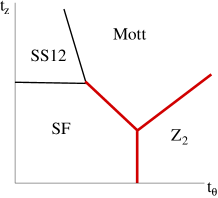
Figure 10: Schematic phase diagram for antiparallel pseudospin vectors. Thick and thin lines have the same meaning as in Fig.9.

Study of various limits and interpolation determines the phase structure of Eq. (86), which is schematically shown in Fig. 10. In addition to the superfluid and Mott states occuring when both $t_{z},t_{\theta}$ are small and large, respectively, there is a supersolid phase, SS12 (it has a minimal unit cell of $12$ sites), and a $Z_{2}$ spin liquid insulating phase. Unlike in the parallel pseudospin model, the SS12 supersolid has the same symmetry as the nearby Mott insulator. This is a direct consequence of the fact that the dual gauge charge is in this case carried by the $U(1)$ degree of freedom $e^{i\theta}$, and this does not carry any space group quantum numbers. For the same reason, the $Z_{2}$ spin liquid phase at large $t_{\theta}$ does not break any symmetries. Note that of the four phases in Fig. 10, only the $Z_{2}$ spin liquid is “exotic”, i.e. has an underlying topological order and unconventional excitations not captured by any local mean-field theory and order parameters.

The excitations are as follows. In the Mott state there are neutral skyrmions (since the $z_{\sigma}$ fields carry no dual gauge charge), confined charge $\pm 1/2$ excitations (visons bound to half-vortices in $z_{\sigma},\theta$), and charge $\pm 1$ excitations that can be viewed as $\pm 4\pi$ vortices in $\theta$. Because $\theta$ is coupled to $A_{i\mu}$, the latter cost finite energy, and are clearly adiabatically connected to vacancy/interstitials in the Mott state. The SS12 phase has the same skyrmion textures, but no well-defined charge excitations since it is a superfluid. Instead, it has a single physical vortex/antivortex excitation created by $e^{\pm i\theta/2}$. The “triviality” of the vortex multiplet is consistent with the broken symmetry of the supersolid, whose enlarged unit cell contains on average an integer number ($6$ in the simplest case) bosons. The $Z_{2}$ spin liquid has physical boson charge $\pm 1/2$ excitations ($2\pi$ vortices in $\theta$ accompanied by a “vison” in $\sigma_{i\mu}$) and physical “vison” excitations (created by $e^{\pm i\theta/2}$ and $z_{\sigma}$) which carry spatial quantum numbers.

The direct transition from superfluid to antiparallel Mott state is described by the continuum action of the previous section. The superfluid-SS12 and the SS12-Mott critical points are also conventional, since each is characterized by a change in a single order parameter. The superfluid-SS12 transition is described by an LGW theory for the ${\bf d}$-vector, while the SS12-Mott transition is simply an XY transition for the superfluid order parameter. The superfluid-$Z_{2}$ transition is also an XY transition, which can be understood as a condensation of charge $\pm 1/2$ “half-bosons” (in principle this changes universal amplitudes from the conventional superfluid to integer-filling Mott transition, which is also XY-likeSedgewick ). The $Z_{2}$ to Mott transition is modeled by the CP¹ action with no gauge field, which has the physical interpretation of modeling vison condensation. We have not attempted to consider the effects of various anisotropies on these transitions.

V Discussion

In this paper we have presented a phenomenological dual vortex theory of the interplay between Mott localization and geometrical frustration for interacting bosons at half-filling on the triangular lattice. This approach reveals a variety of novel quantum phases and phase transitions which may occur if the superfluid and Mott insulating states occur in close proximity to one another in phase space. Of particular interest are the continuous superfluid-Mott insulator transition predicted by mean field theory, the two supersolid phases, and the occurrence of the recently-discovered NCCP¹ critical universitality class at the 3-sublattice supersolid to Mott insulator transition. In this discussion, we will provide a more direct physical picture of some of these phenomena, and address the prospects of observing them in simple microscopic boson or spin models.

A useful starting point for the discussion is the recent demonstration that a supersolid phase indeed occurs in the simplest spin-$1/2$ XXZ model,

$$H_{XXZ}=\sum_{\langle ij\rangle}-J_{\perp}(S_{i}^{x}S_{j}^{x}+S_{i}^{y}S_{j}^{y})+J_{z}S_{i}^{z}S_{j}^{z},$$ (87)

with ferromagnetic XY and antiferromagnetic Ising exchanges ($J_{\perp},J_{z}>0$) (equivalently, hard-core bosons with nearest neighbor repulsion) on nearest-neighbor links of the triangular lattice.Melko05 ; Damle05 ; Troyer05 This model was shown to be in a 3-sublattice SS3-type phase for $J_{z}\gtrsim 5J_{\perp}$, and this phase persists up to and including $J_{z}=\infty$. A number of features of the numerical results on the supersolid at large $J_{z}$ are notable. First, although superfluidity survives, it is extremely weak, as characterized by the superfluid stiffness, which is approximately $250$ times smaller in the large $J_{z}$ supersolid than in the pure XY model ($J_{z}=0$). Second, it is exceedingly difficult to distinguish numerically on even relatively large lattices between the two different types of SS3 charge ordering patterns. Ref. Melko05,  was unable to distinguish them numerically by direct measurement of boson density correlation functions, while Ref. Damle05,  claimed to do so, but only for large lattices of $18\times 18$ sites with a very small signal. Furthermore, a deviation of the density from half-filling is expectedMelko05  in the “ferrimagnetic” SS3 phase identified in Ref. Damle05,  (which corresponds in our theory to the one with $w_{3}<0$), but appears to be exceedingly minute if observable at all computationally. Apparently there is very little splitting energetically between the two SS3 states, even at $J_{z}=\infty$, a point at which there is no intrinsic small parameter in the microscopic Hamiltonian – the effective Hamiltonian is simply the XY exchange projected into the Hilbert space spanned by the manifold of classical Ising antiferromagnetic ground states on the triangular lattice.

The present theory offers a partial explanation for these puzzling observations. We interpret the weakness of superfluidity as evidence that the system is in close proximity to a Mott insulating state. If so, our dual vortex field theory, which is built around a superfluid to Mott insulating transition, should apply. The tiny energy splitting between the two SS3 states is then understandable: the term which dictates this splitting, $w_{3}$ is $12^{\rm th}$ order in the basic $z_{\pm\sigma}$ vortex fields, and clearly strongly irrelevant at the superfluid-Mott QCP. Furthermore, the smallness of any spontaneous density deviation from $1/2$-filling, which as indicated above is expected for the “ferrimagnetic” SS3 state, is also expected, since the density deviation must vanish as the Mott state, which has density of exactly $1/2$ and is incompressible, is approached. This deviation also vanishes at the transition from this state to the superfluid (as seen in LGW theoryMelko05 ), so it is likely small throughout the ferrimagnetic phase.

Given these arguments for proximity to the Mott state, it seems likely that only a small perturbation of the XXZ Hamiltonian may be required to push it into a Mott phase, and in so doing observe the very interesting NCCP¹ criticality at the SS3-Mott quantum critical point. Let us try to develop a more physical picture of this transition. We will begin by providing a cartoon understanding of the SS3 phases. In the case $w_{3}<0$, as discussed in Refs. Damle05, ; Troyer05, , the ferrimagnetic SS3 state can be understood crudely by first forming a “solid” of bosons with a density of $1/3$, with one boson occupying each of the sites of one of the three $\sqrt{3}\times\sqrt{3}$ triangular sublattices of the original lattice. This leaves, at $f=1/2$, a density of $1/4$ boson per the remaining sites, which form a honeycomb lattice, with the “solid” bosons in the centers of the honeycomb plaquettes. The SS3 state can be viewed as a superfluid of these remaining bosons (alternatively, one can make the same construction with holes replacing bosons, leading to a different but equivalent state – which illustrates the spontaneously broken particle-hole symmetry of the ferrimagnet). In the opposite case $w_{3}>0$, there is no spontaneous density polarization, and the “sublattice magnetizations” take the values $\langle S_{i}^{z}\rangle=(m,-m,0)$ on the three inequivalent sites. We will call this the “antiferromagnetic” state because of the exactly opposite Ising moments on two of the three sublattices. This state can be understood by a similar cartoon. In particular, take a honeycomb sublattice of the triangular lattice, and on this sublattice form a $1/2$-filled Mott insulator of alternating empty and occupied sites (an Ising Néel state in spin language). The sites at the centers of the honeycomb plaquettes form a $\sqrt{3}\times\sqrt{3}$ triangular sublattice, and we put the remaining bosons into a half-filled superfluid on this sublattice. These cartoon pictures would clearly tend to favor the ferrimagnetic state in the XXZ model, since bosons must hop (presumably virtually) between second neighbor sites to stabilize the triangular superfluid in the antiferromagnetic state. This immediately suggests that, to study the antiferromagnetic supersolid, one needs only to add a second neighbor XY exchange to the XXZ model,

$$H^{\prime}=-J^{\prime}_{\perp}\sum_{\langle\langle ij\rangle\rangle}S_{i}^{x}S_{j}^{x}+S_{i}^{y}S_{j}^{y}.$$ (88)

With these pictures of the SS3 phases in hand, it is natural to view the transition to the Mott insulator as a “crystallization” of the superfluid sublattices of the supersolid. Indeed, we find that this provides a simple physical picture consistent with the symmetries of the appropriate Mott phases. Consider first the transition from the ferrimagnet. Here we have a $1/4$-filled honeycomb lattice of bosons, which is to undergo a superfluid to Mott insulator transition. At $1/4$-filling, these bosons are unlikely to form a simple “crystalline” Mott insulator, since they would be too widely separated to substantially interact. Instead, more likely Mott states are valence bond solids, in which the bosons resonate between two or more sites (within still-localized wavefunctions). The most natural candidate is a “columnar” valence bond solid (VBS) state, in which alternating columns of bonds are occupied by one boson. Indeed, the state predicted by the vortex mean field theory for $w_{3}<0$ and $w_{2}<0$ has exactly the symmetries of the columnar valence bond solid, see Fig. 11. One may also convince oneself of the validity of the columnar VBS picture by counting the number of distinct Mott states. Fix the location of the $\sqrt{3}\times\sqrt{3}$ superlattice and hence the honeycomb sublattice. One can then place the valence bonds along columns parallel to any of the three principle axes (of the honeycomb, which has principle axes halfway between those of the underlying triangular lattice), and for each such orientation, they may lie on even or odd columns. Hence one expects six states. This is precisely the number of distinct choices of vector pseudospin along the $\pm\hat{x},\pm\hat{y},\pm\hat{z}$ axes.

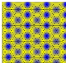
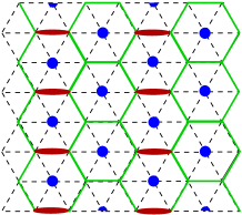
Figure 11: Density plot for the ferrimagnetic solid (left) and the corresponding cartoon (right). In the density plot, the honeycomb sublattice is clearly visible. In the cartoon, the honeycomb lattice on which the superfluid lives is overlaid in green, with the frozen bosons in blue, and the valence bonds that form on passing from the ferrimagnetic SS3 phase to the ferrimagnetic solid are drawn as red ovals (color online).

Next consider the antiferromagnetic supersolid. We have an effective $\sqrt{3}\times\sqrt{3}$ triangular sublattice of bosons at half-filling, living in the plaquette centers of an “antiferromagnetic” bose solid on the honeycomb lattice. In the absence of this surrounding solid, the triangular sublattice would have, scaled up to its size, all the same symmetries as the original triangular lattice. The formation of a Mott insulator on this triangular sublattice would thus naïvely appear to be just as formidable a problem as the original one. The staggered solid, however, breaks $I_{d_{2}}$ and $C$, preserving only the combination, $I_{d_{2}}\circ C$. This means, were we to repeat the PSG analysis for a dual vortex theory of the $\sqrt{3}\times\sqrt{3}$ sublattice bosons, there is no symmetry to prevent the Ising order parameter $\Phi=|z_{+}|^{2}-|z_{-}|^{2}$ from appearing as a term in the action, breaking the $\alpha=\pm$ “flavor” degeneracy of the vortex multiplet. Clearly in such a theory, then only one of the two flavors will condense, and only those phases in which one pseudospin is non-zero will appear. Incidentally, one may identify therefore the $z_{\sigma}$ spinor in the hard-spin action with the lower-energy vortex flavor in this sublattice theory. The phases with only a single pseudospin condensed are “staggered” phases of the original bosons. The simplest of these is just a “columnar crystal”, in which bosons on alternating columns of triangular lattice sites (along some principle axis) are occupied and unoccupied. Superimposing this upon the surrounding antiferromagnetic honeycomb lattice, one remarkably obtains an ordering pattern again identical in symmetry to the original mean-field solid with $w_{3}>0$ and $w_{2}<0$! The counting of states is also the same as for the ferrimagnetic case above, since the “columns” have the same set of orientations and have only shifted from bonds to sites, once again in agreement with the configurations of ${\bf S}$.

One can easily extend these constructions to the cases with pseudospin along (111). For brevity, we relegate this to Appendix E.

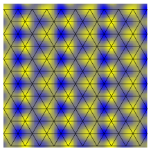
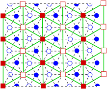
Figure 12: Density plot for the antiferromagnetic solid (left) and the corresponding cartoon (right). In the cartoon, the triangular lattice on which the superfluid lives is overlaid in green, with the crystallized bosons/vacancies forming the Mott insulating honeycomb lattice in blue (filled and empty circles). The additional bosons/vacancies that solidify on passing from the antiferromagnetic SS3 phase to the antiferromagnetic solid are drawn as red squares (filled and empty, respectively).

The cartoons of the ferrimagnetic and antiferromagnetic supersolids/solids not only reproduce the symmetries of the phases, but also can be directly used to obtain the critical NCCP¹ theory of the SS3-Mott transition. In the ferrimagnetic case, the cartoon picture is a superfluid-Mott transition on a $1/4$-filled honeycomb lattice of bosons. In Appendix F, we sketch how a dual vortex analysis of that “cartoon” problem directly recovers the appropriate NCCP¹ theory for this case. In the antiferromagnetic case, a similar argument has already been sketched for the cartoon of an half-filled triangular $\sqrt{3}\times\sqrt{3}$ sublattice in the background of the honeycomb antiferromagnetic Mott state, which removes one of the two pseudospinors from the theory, likewise recovering the NCCP¹ model and the appropriate anisotropy.

It thus seems of considerable interest to pursue small perturbations of the XXZ model which might take it into a Mott phase, and between ferrimagnetic and antiferromagnetic states. To make the latter transition, from the ferrimagnetic to antiferromagnetic SS3 supersolid, we can make a simple recommendation: the inclusion of weak second-neighbor ferromagnetic exchange, as in Eq. (88), should favor the antiferromagnetic state by allowing bosons to better move on the triangular sublattice. The antiferromagnetic states seem slightly more favorable than the ferrimagnetic ones theoretically as candidates for observing the NCCP¹ criticality, because the latter preserve particle-hole symmetry in the supersolid, and have weaker pseudospin anisotropy terms. Understanding what terms microscopically would be needed to push the XXZ model toward the insulators is a nontrivial problem. However, it seems clear that introducing further-neighbor Ising exchange will lead to some Mott insulating states, when $J_{z}$ is large, since they spoil the degeneracy of the classical Ising manifold. Exploration of this problem numerically is tempting.

Analytically, it is quite interesting how naturally the dual vortex approach leads to the observed supersolid states. Coming from the Mott insulator with parallel pseudospins, the deconfined charge excitations are skyrmions. If one imagines lowering the charge gap in the insulator, it is most natural that these should condense, destroying the pseudospin order of the insulator and simultaneously initiating superfluidity. While other scenarios such as the direct Mott insulator to superfluid transition are possible theoretically (and described analytically in this paper), they entail a non-trivial screening so that confinement of other (fractionally charged) excitations of the Mott state becomes progressively weaker as the transition is approached. Thus the SS3 supersolid is probably the most intuitive “neighbor” of the Mott state, and with this understanding its occurence in the strong interaction limit of the XXZ model is no longer surprising. It is interesting to speculate as to whether it might be possible to formulate the boson-vortex duality used heavily in this paper directly in this strong-coupling region, i.e. in the classical Ising antiferromagnetic Hilbert space. Such a formulation could potentially provide a quantitative method for attacking problems of Mott transitions with strong frustration.

Appendix A Various PSG details

The PSG transformations in momentum space are given by:

$$T_{1} : \left\{\begin{array}[]{ccl}\psi_{1}(k_{1},k_{2})&\rightarrow&\psi_{1}(k_{1},k_{2}-2\pi f)e^{-ik_{1}}\\ \psi_{2}(k_{1},k_{2})&\rightarrow&\psi_{2}(k_{1},k_{2}-2\pi f)e^{-ik_{1}}\omega\end{array}\right.,$$ (91)

$$T_{2} : \left\{\begin{array}[]{ccl}\psi_{1}(k_{1},k_{2})&\rightarrow&\psi_{1}(k_{1},k_{2})e^{-ik_{2}}\\ \psi_{2}(k_{1},k_{2})&\rightarrow&\psi_{2}(k_{1},k_{2})e^{-ik_{2}}\end{array}\right.,$$ (94)

$$R_{2\pi/3} : \left\{\begin{array}[]{ccl}\psi_{1}(k_{1},k_{2})&\rightarrow&\frac{1}{q}\sum_{m,n=0}^{q-1}\omega^{m(m+2n+\nu_{q})/2}\psi_{1}(k_{2}+2\pi fm,-k_{1}-k_{2}+2\pi f(n-1/2+\nu_{q}/2))\\ \psi_{2}(k_{1},k_{2})&\rightarrow&\frac{1}{q}e^{i(k_{1}+k_{2})}\sum_{m,n=0}^{q-1}\omega^{(m-1)(m+2n-1+\nu_{q})/2}\psi_{2}(k_{2}+2\pi fm,-k_{1}-k_{2}+2\pi f(n-1/2+\nu_{q}/2))\end{array}\right.,$$ (97)

$$I_{d_{1}} : \left\{\begin{array}[]{ccl}\psi_{1}(k_{1},k_{2})&\rightarrow&\frac{1}{q}\sum_{m,n=0}^{q-1}\psi_{1}^{*}(k_{2}+2\pi fm,k_{1}+2\pi fn)\omega^{-mn}\\ \psi_{2}(k_{1},k_{2})&\rightarrow&\frac{1}{q}e^{i(k_{1}+k_{2})}\sum_{m,n=0}^{q-1}\psi_{2}^{*}(k_{2}+2\pi fm,k_{1}+2\pi fn)\omega^{-(m-1)n}\end{array}\right.,$$ (100)

$$I_{d_{2}} : \left\{\begin{array}[]{ccl}\psi_{1}(k_{1},k_{2})&\rightarrow&\frac{1}{q}e^{-ik_{1}}\sum_{m,n=0}^{q-1}\psi_{2}^{*}(-k_{2}+2\pi fm,-k_{1}+2\pi fn)\omega^{-(m-1)n}\\ \psi_{2}(k_{1},k_{2})&\rightarrow&\frac{1}{q}e^{ik_{2}}\sum_{m,n=0}^{q-1}\psi_{1}^{*}(-k_{2}+2\pi fm,-k_{1}+2\pi fn)\omega^{-mn}\end{array}\right.,$$ (103)

where $\nu_{q}=q-2[q/2]$.

Using these general forms for the PSG in momentum space, it is straightforward to obtain Eqs. (II,II) of the main text. The remaining PSG transformations for the multiplets are:

$$R_{2\pi/3}:\varphi_{\ell}\rightarrow\frac{1}{\sqrt{q}}\sum_{\ell^{\prime}=0}^{q-1}\omega^{-\ell(\ell+2\ell^{\prime}+1)/2}\varphi_{\ell^{\prime}},$$

$$I_{d_{1}}:\varphi_{\ell}\rightarrow\frac{1}{\sqrt{q}}\sum_{\ell^{\prime}=0}^{q-1}\omega^{\ell\ell^{\prime}}\varphi^{*}_{\ell^{\prime}},$$

$$I_{d_{2}}:\varphi_{\ell}\rightarrow\frac{1}{\sqrt{q}}\sum_{\ell^{\prime}=0}^{q-1}\omega^{-\ell\ell^{\prime}}\varphi^{*}_{\ell^{\prime}},$$ (104)

for $q$ odd, and

$$R_{2\pi/3}:\varphi_{\alpha\sigma}\rightarrow e^{-i\pi\alpha\sigma/q}\frac{e^{i\eta_{1}(\alpha,f)}}{\sqrt{q}}\sum_{\sigma^{\prime}=0}^{q-1}\omega^{-\sigma(\sigma+2\sigma^{\prime}+1)/2}\varphi_{\alpha\sigma^{\prime}},$$

$$I_{d_{1}}:\varphi_{\alpha\sigma}\rightarrow\frac{e^{i\eta_{2}(\alpha,f)}}{\sqrt{q}}\sum_{\sigma^{\prime}=0}^{q-1}\omega^{\sigma\sigma^{\prime}}\varphi^{*}_{\alpha\sigma^{\prime}},$$

$$I_{d_{2}}:\varphi_{\alpha\sigma}\rightarrow\frac{e^{i\eta_{3}(\alpha,f)}}{\sqrt{q}}\sum_{\sigma^{\prime}=0}^{q-1}\omega^{-\sigma\sigma^{\prime}}\varphi^{*}_{-\alpha,\sigma^{\prime}},$$ (105)

when $q$ is an even integer. Appying $R_{2\pi/3}$ to $\tilde{\varrho}^{\alpha}_{mn}$, one finds that

$$\eta_{1}(\alpha)=-\frac{\pi\alpha}{6q}.$$ (106)

Applying $I_{d_{2}}$, one finds that $\eta_{3}(\alpha)=0$. The remaining phase factor $\eta_{2}(\alpha,f)$ is difficult to find analytically in the general case. In the case $f=1/2$ considered in detail in the text, it is, however, equal to $\eta_{1}(\alpha)$, so collecting these results,

$$\eta_{1}(\alpha)=\eta_{2}(\alpha)=-\pi\alpha/12,\,\,\,\eta_{3}(\alpha)=0\qquad\mbox{for $f=1/2$}.$$ (107)

It is possible that $\eta_{1}(\alpha)=\eta_{2}(\alpha)$ holds at a general filling, not just at $f=1/2$, but it is not obvious.

For the specific case of $f=1/2$ ($p=1,q=2$), we can impose invariance under the particle-hole transformation,

$$C\,:\,\varphi_{\pm\sigma}\rightarrow\varphi^{*}_{\mp\sigma}.$$ (108)

Imposing invariance under the rotation and reflection operations above upon the quartic action ${\cal L}_{1}$ taken in the form of Eq. (28) yields the set of conditions

$$\gamma_{mn}=\gamma_{-m,-n},$$

$$\gamma_{mn}=\gamma_{m,m-n},$$

$$\gamma_{mn}=\gamma_{m-2n,-n}^{*},$$

$$\gamma_{m^{\prime}n^{\prime}}=\frac{1}{q}\sum_{m,n=0}^{q-1}\gamma_{mn}\omega^{mn^{\prime}-nm^{\prime}},$$

$$\gamma_{m^{\prime}n^{\prime}}=\frac{1}{q}\sum_{m,n=0}^{q-1}\gamma_{mn}\omega^{n(m^{\prime}-n-2n^{\prime})+m(n+n^{\prime})},$$

for $q$ odd, and

$$\gamma_{mn}^{\alpha\beta}=\gamma_{-m,-n}^{-\alpha-\beta},$$

$$\gamma_{mn}^{\alpha\beta}=\gamma_{-m,-n}^{\beta\alpha},$$

$$\gamma_{mn}^{\alpha\beta}=\gamma_{m-2n,-n}^{\alpha\beta*},$$

$$\gamma_{m^{\prime}n^{\prime}}^{\alpha\beta}=\frac{1}{q}\sum_{m,n=0}^{q-1}\gamma_{mn}^{\alpha\beta}\omega^{mn^{\prime}-nm^{\prime}},$$

$$\gamma^{\alpha\beta}_{m^{\prime}n^{\prime}}=\frac{1}{q}\sum_{m,n=0}^{q-1}\gamma_{mn}^{\alpha\beta}e^{i\pi n(\beta-\alpha)/q}\omega^{n(m^{\prime}-n-2n^{\prime})+m(n+n^{\prime})},$$

for $q$ even.

Appendix B Pseudospin transformations at $f=1/2$

For convenience, we give the transformation properties of the spinor $z_{\alpha\sigma}$ vortex fields. With the pseudospin index suppressed, we find

$$T_{1} : \left\{\begin{array}[]{lcr}z_{+}&\rightarrow&e^{-i\pi/6}\tau^{x}z_{+}\\ z_{-}&\rightarrow&-e^{i\pi/6}\tau^{x}z_{-}\end{array}\right.,$$ (113)

$$T_{2} : \left\{\begin{array}[]{lcr}z_{+}&\rightarrow&e^{-i\pi/6}\tau^{z}z_{+}\\ z_{-}&\rightarrow&-e^{i\pi/6}\tau^{z}z_{-}\end{array}\right.,$$ (116)

$$R_{2\pi/3} : \left\{\begin{array}[]{lcr}z_{+}&\rightarrow&e^{-i\pi/3}u_{r}z_{+}\\ z_{-}&\rightarrow&e^{i\pi/3}u_{r}z_{-}\end{array}\right.,$$ (119)

$$I_{d_{1}} : \left\{\begin{array}[]{lcr}z_{+}&\rightarrow&e^{i5\pi/12}u_{\scriptscriptstyle 1}^{\vphantom{*}}z^{*}_{+}\\ z_{-}&\rightarrow&e^{-i5\pi/12}u_{\scriptscriptstyle 1}^{\vphantom{*}}z^{*}_{-}\end{array}\right.,$$ (122)

$$I_{d_{2}} : \left\{\begin{array}[]{lcr}z_{+}&\rightarrow&iu_{\scriptscriptstyle 2}^{\vphantom{*}}z^{*}_{-}\\ z_{-}&\rightarrow&iu_{\scriptscriptstyle 2}^{\vphantom{*}}z^{*}_{+}\end{array}\right.,$$ (125)

$$C : \left\{\begin{array}[]{lcr}z_{+}&\rightarrow&-\epsilon z_{-}^{*}\\ z_{-}&\rightarrow&\epsilon z^{*}_{+}\end{array}\right..$$ (128)

Here

$$u_{r} = e^{i\frac{\pi}{3}{\boldsymbol{\hat{n}}}_{r}\cdot{\boldsymbol{\tau}}}=\frac{1}{2}\left(\begin{array}[]{cc}1+i&1+i\\ -1+i&1-i\end{array}\right),$$ (131)

$$u_{1} = e^{-i\frac{\pi}{2}{\boldsymbol{\hat{n}}}_{1}\cdot{\boldsymbol{\tau}}}=\frac{1}{\sqrt{2}}\left(\begin{array}[]{cc}-i&-i\\ -i&i\end{array}\right),$$ (134)

$$u_{2} = e^{i\frac{\pi}{2}{\boldsymbol{\hat{n}}}_{2}\cdot{\boldsymbol{\tau}}}=\frac{1}{\sqrt{2}}\left(\begin{array}[]{cc}-i&i\\ i&i\end{array}\right),$$ (137)

with

$${\boldsymbol{\hat{n}}}_{r} = (1,1,1)/\sqrt{3},$$

$${\boldsymbol{\hat{n}}}_{1} = (1,0,1)/\sqrt{2},$$

$${\boldsymbol{\hat{n}}}_{2} = (1,0,-1)/\sqrt{2}.$$ (138)

Next we tabulate the transformation properties of the pseudospin vector order parameters:

$$T_{1} : \left\{\begin{array}[]{lcr}S_{\alpha}^{x}&\rightarrow&S_{\alpha}^{x}\\ S_{\alpha}^{y}&\rightarrow&-S_{\alpha}^{y}\\ S_{\alpha}^{z}&\rightarrow&-S_{\alpha}^{z}\end{array}\right.,$$ (142)

$$T_{2} : \left\{\begin{array}[]{lcr}S_{\alpha}^{x}&\rightarrow&-S_{\alpha}^{x}\\ S_{\alpha}^{y}&\rightarrow&-S_{\alpha}^{y}\\ S_{\alpha}^{z}&\rightarrow&S_{\alpha}^{z}\end{array}\right.,$$ (146)

$$R_{2\pi/3} : \left\{\begin{array}[]{lcr}S_{\alpha}^{x}&\rightarrow&S_{\alpha}^{y}\\ S_{\alpha}^{y}&\rightarrow&S_{\alpha}^{z}\\ S_{\alpha}^{z}&\rightarrow&S_{\alpha}^{x}\end{array}\right.,$$ (150)

$$I_{d_{1}} : \left\{\begin{array}[]{lcr}S_{\alpha}^{x}&\rightarrow&S_{\alpha}^{z}\\ S_{\alpha}^{y}&\rightarrow&S_{\alpha}^{y}\\ S_{\alpha}^{z}&\rightarrow&S_{\alpha}^{x}\end{array}\right.,$$ (154)

$$I_{d_{2}} : \left\{\begin{array}[]{lcr}S_{\alpha}^{x}&\rightarrow&-S_{-\alpha}^{z}\\ S_{\alpha}^{y}&\rightarrow&S_{-\alpha}^{y}\\ S_{\alpha}^{z}&\rightarrow&-S_{-\alpha}^{z}\end{array}\right.,$$ (158)

$$C : {\bf S}_{\alpha}\rightarrow-{\bf S}_{-\alpha}.$$ (159)

Appendix C Hard spin tranformations

Here we give the transformation rules for the hard-spin theory with parallel pseudospins. Defining

$$z_{\pm}=ze^{\pm i\theta/2},$$ (160)

we obtain

$$T_{1} : \left\{\begin{array}[]{lcr}z&\rightarrow&i\tau^{x}z\\ \theta&\rightarrow&\theta-4\pi/3\end{array}\right.,$$ (163)

$$T_{2} : \left\{\begin{array}[]{lcr}z&\rightarrow&i\tau^{z}z\\ \theta&\rightarrow&\theta-4\pi/3\end{array}\right.,$$ (166)

$$R_{2\pi/3} : \left\{\begin{array}[]{lcr}z&\rightarrow&u_{r}z\\ \theta&\rightarrow&\theta-2\pi/3\end{array}\right.,$$ (169)

$$I_{d_{1}} : \left\{\begin{array}[]{lcr}z&\rightarrow&u_{\scriptscriptstyle 1}^{\vphantom{*}}z^{*}\\ \theta&\rightarrow&5\pi/6-\theta\end{array}\right.,$$ (172)

$$I_{d_{2}} : \left\{\begin{array}[]{lcr}z&\rightarrow&u_{\scriptscriptstyle 2}^{\vphantom{*}}z^{*}\\ \theta&\rightarrow&\theta\end{array}\right.,$$ (175)

$$C : \left\{\begin{array}[]{lcr}z&\rightarrow&\epsilon z^{*}\\ \theta&\rightarrow&\theta+\pi.\end{array}\right.$$ (178)

The $SU(2)$ matrices $u$ are defined in Eqs. (131). We have used the freedom to redefine any of these operations by a global $U(1)$ gauge transformation, which in this hard-spin limit corresponds to a phase rotation of $z$.

Appendix D Residual symmetries of the SS2 supersolid

The residual symmetry operations of this SS2 state (which are not broken by the pseudospin vector order) are generated by $T_{1}$, $R_{2\pi/3}\circ I_{d_{1}}$, $C\circ I_{d_{2}}\circ I_{d_{1}}$, and $T_{2}\circ I_{d_{2}}\circ I_{d_{1}}$. Their action on the $z_{\pm}$ vortex fields can be obtained from the definition $z_{\pm\sigma}=z_{\pm}\eta_{\sigma}$ and Eqs. (113):

$$T_{1} : z_{\pm}\rightarrow\pm e^{\mp i\pi/6}z_{\pm},$$

$$R_{2\pi/3}\circ I_{d_{1}} : \left\{\begin{array}[]{ccc}z_{+}&\rightarrow&z_{+}^{*}\\ z_{-}&\rightarrow&iz_{-}^{*}\end{array}\right.$$ (182)

$$C\circ I_{d_{2}}\circ I_{d_{1}} : z_{\pm}\rightarrow e^{\mp i\pi/12}z_{\pm}^{*},$$

$$T_{2}\circ I_{d_{2}}\circ I_{d_{1}} : z_{\pm}\rightarrow-e^{\pm i\pi/12}z_{\mp}.$$ (183)

These lead directly to Eq. (85).

Appendix E Toy model wavefunctions with (111) pseudospin

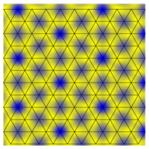
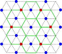
Figure 13: Density plot for the ferrimagnetic solid (left) and the corresponding cartoon (right) with (111) pseudospin ordering.

Here we provide toy model wavefunctions for the Mott states with $w_{2}>0$ and parallel pseudospins, so that ${\bf S}_{+}={\bf S}_{-}$ lies along say the $(111)$ axis. First consider $w_{3}>0$, in which we wish to construct a state appropriate to a $1/4$-filled honeycomb lattice. In this case, a wavefunction with the correct symmetry is shown in Fig.13. In this figure the bosons denoted by squares are on the honeycomb sublattice of the triangular lattice, and become superfluid in the SS3 phase.

Now consider $w_{3}<0$, in which case we must consider the half-filled triangular lattice embedded in the antiferromagnetic honeycomb Mott insulator. The density plot for this state is shown in Fig.14. Focusing on the triangular lattice sites, we note that the amplitude on these sites has the same $2\times 2$ periodicity as the $w_{3}>0$ state above, with the sites on this sublattice having one amplitude, and the remaining sites another. However, it is inconsistent with half-filling to simply put one boson on the sublattice sites, or on the other three sites. Moreover, the state is rather constrained by the existence of a number of centers of three-fold rotations and reflections. The simplest Mott wavefunction we constructed that satisfies all symmetry properties is actually not quite a product state of the form of Eq. (39). It is, however, clearly an insulating state. To construct it, assume the $2\times 2$ sublattice sites are empty. Then the remaining sites form a kagome lattice. The kagome lattice is composed of corner-sharing triangles, or two orientations (pointing “left” and “right” in the figure). We act with creation operators to place one boson on each triangle in a uniform superposition.

$$\Psi=\prod_{\triangle}(b_{\triangle 1}^{\dagger}+b_{\triangle 2}^{\dagger}+b_{\triangle 3}^{\dagger})|0\rangle$$ (184)

Since the triangles overlap, there will actually be amplitude to find more than one boson per triangle. On average, the number of bosons per unit cell of the kagome lattice is then $2$, since there is one up and one down triangle per unit cell. There are four triangular lattice sites for each such unit cell (3 kagome and one central empty site), so this is a state at $1/2$-filling, which manifestly has all the symmetries of the Mott state in Fig.14. Moreover, it is an insulating state as required, since one can readily show there are only very short-range correlations, e.g. in the boson Green’s function.

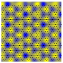
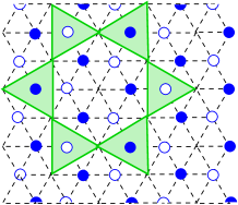
Figure 14: Density plot for the antiferromagnetic solid (left) and the corresponding cartoon (right) with (111) pseudospin ordering.

Appendix F Honeycomb lattice at $1/4$-filling

The vortex PSG’s on the honeycomb lattice were worked out in Appendix B of the first paper in Ref. Balents04, . They are sufficient to develop a dual vortex theory of the superfluid-Mott transition on this lattice. For the case of $f=1/4$, there are two vortex flavors, $\varphi_{0},\varphi_{1}$, which can be combined into a spinor $\varphi_{\sigma}$. We consider the restrictions upon the vortex Lagrangian by translations and rotations. Suppressing the indices and using Pauli matrices ${\boldsymbol{\tau}}_{\sigma\sigma^{\prime}}$ to span the spinor space, we have:

$$T_{1} : \varphi\rightarrow\tau^{x}\varphi,$$

$$T_{2} : \varphi\rightarrow\tau^{z}\varphi,$$

$$T_{d} : \varphi\rightarrow\tau^{y}\varphi,$$

$$R^{\rm dual}_{2\pi/3} : \varphi\rightarrow e^{-i\pi/3}u_{r}\varphi,$$ (185)

where $u_{r}$ is given in Eq. (131). Requiring invariance under these PSG operations, one may readily write down a continuum Lagrangian in terms of $\varphi$:

$${\cal L}_{\rm honey} = \sum_{\sigma=0,1}\left[|(\partial_{\mu}-iA_{\mu})\varphi_{\sigma}|^{2}+s|\varphi_{\sigma}|^{2}\right]+u(\varphi_{\sigma}^{*}\varphi_{\sigma}^{\vphantom{*}})^{2}$$ (186)

$$+ \frac{1}{2e^{2}}(\epsilon_{\mu\nu\lambda}\partial_{\nu}A_{\lambda})^{2}+{\cal L}_{a},$$

where $SU(2)$ symmetry of $\varphi_{\sigma}$ is first broken by the term

$${\cal L}_{a}=\lambda S^{x}S^{y}S^{z},$$ (187)

with ${\bf S}=\varphi_{\sigma}^{*}{\boldsymbol{\tau}}_{\sigma\sigma^{\prime}}\varphi_{\sigma}$. Eq. (186) indeed has the global $SU(2)$ and $U(1)$ gauge symmetry of the NCCP¹ model, and ${\cal L}_{a}$ recovers the leading anisotropy term in Eq. (82) for the ferrimagnetic case.

References

- (1) M. Greiner, O. Mandel, T. Esslinger, T.W. Hansch, and I. Bloch, Nature 415, 39 (2002).
- (2) C. Urano, M. Nohara, S. Kondo, F. Sakai, H. Takagi, T. Shiraki, and T. Okubo, Phys. Rev. Lett. 85, 1052 (2000); S.H. Lee, Y. Qiu, C. Broholm, Y. Ueda, and J.J. Rush, Phys. Rev. Lett. 86, 5554 (2001); A. Koda, R. Kadono, W. Higemoto, K. Ohishi, H. Ueda, S. Urano, S. Kondo, M. Nohara, and H. Takagi, Phys. Rev. B 69, 012402 (2004).
- (3) A. Fang, C. Howald, N. Kaneko, M. Greven, and A. Kapitulnik, cond-mat/0404452 (unpublished); M. Vershinin, S. Misra, S. Ono, Y. Abe, Y. Ando, and A. Yazdani, Science 303, 1995 (2004); K. McElroy, D.H. Lee, J.E. Hoffman, K.M. Lang, E.W. Hudson, H. Eisaki, S. Uchida, J. Lee, and J.C. Davis, cond-mat/0404005 (unpublished); X.F. Sun, K. Segawa, and Y. Ando, cond-mat/0502223 (unpublished).
- (4) L.-M. Duan, E. Demler, and M.D. Lukin, Phys. Rev. Lett. 91, 090402 (2003).
- (5) D. Jaksch, and P. Zoller, cond-mat/0410614 (unpublished).
- (6) H.P. Büchler, M. Hermele, S.D. Huber, M.P.A. Fisher, and P. Zoller, cond-mat/0503254 (unpublished).
- (7) T. Senthil, A. Vishwanath, L. Balents, S. Sachdev, and M.P.A. Fisher, Science 303, 1490 (2004); T. Senthil, L. Balents, A. Vishwanath, S. Sachdev, and M.P.A. Fisher, Phys. Rev. B 70, 144407 (2004).
- (8) L. Balents, L. Bartosch, A. Burkov, S. Sachdev, and K. Sengupta, Phys. Rev. B 71, 144508 (2005); ibid. 71, 144509 (2005); L. Bartosch, L. Balents and S. Sachdev, cond-mat/0502002 (unpublished).
- (9) L. Balents, L. Bartosch, A. Burkov, S. Sachdev, and K. Sengupta, cond-mat/0504692 (unpublished).
- (10) R.G. Melko, A. Paramekanti, A.A. Burkov, A. Vishwanath, D.N. Sheng, and L. Balents, cond-mat/0505258 (unpublished).
- (11) D. Heidarian and K. Damle, cond-mat/0505257 (unpublished).
- (12) S. Wessel and M. Troyer, cond-mat/0505298 (unpublished).
- (13) A.F. Andreev and I.M. Lifshitz, Sov. Phys. JETP 29, 1107 (1969); G. Chester, Phys. Rev. A 2, 256 (1970); A.J. Leggett, Phys. Rev. Lett. 25, 1543 (1970); K.-S. Liu and M.E. Fisher, J. Low Temp. Phys. 10, 655 (1973).
- (14) A.W. Sandvik, S. Daul, R.R.P. Singh, and D.J. Scalapino, Phys. Rev. Lett. 89, 247201 (2002).
- (15) O.I. Motrunich, and A. Vishwanath, Phys. Rev. B 70, 075104 (2004).
- (16) M. Oshikawa, Phys. Rev. Lett. 84, 1535-1538 (2000).
- (17) M.B. Hastings, Phys. Rev. B 69, 104431 (2004).
- (18) Xiao-Gang Wen, Int. J. Mod. Phys. B4, 239 (1990).
- (19) J.B. Kogut, Rev. Mod. Phys. 51, 659 (1979).
- (20) C. Lannert, M.P.A. Fisher, and T. Senthil, Phys. Rev. B 63, 134510 (2001).
- (21) L. Balents, M.P.A. Fisher, and C. Nayak, Phys. Rev. B 60, 1654 (1999).
- (22) T. Senthil, and M.P.A. Fisher, Phys. Rev. B 62, 7850 (2000).
- (23) Xiao-Gang Wen, Phys. Rev. B 44, 2664 (1991).
- (24) D.R. Nelson, Phys. Rev. Lett. 60, 1415 (1988); D.R. Nelson and S. Seung, Phys. Rev. B 39, 9153 (1989).
- (25) R.D. Sedgewick, D.J. Scalapino, and R.L. Sugar, Phys. Rev. B 65, 54508 (2002).