Quantum state tomography with quantum shotnoise

Abstract

We propose a scheme for a complete reconstruction of one- and two-particle orbital quantum states in mesoscopic conductors. The conductor in the transport state continuously emits orbital quantum states. The orbital states are manipulated by electronic beamsplitters and detected by measurements of average currents and zero frequency current shotnoise correlators. We show how, by a suitable complete set of measurements, the elements of the density matrices of the one- and two-particle states can be directly expressed in terms of the currents and current correlators.

According to the standard interpretation of quantum mechanics the wavefunction, or more generally the density matrix, determines the probabilities for the possible outcomes of any measurement on the quantum state. To completely characterize the wavefunction of the state is therefore of fundamental interest Pauli . It is however impossible to infer anything about an unknown state from a single measurement, a complete characterization requires an ensemble of identically prepared states and the measurement of a complete set of observables on the state Fano . A reconstruction of the quantum state wavefunction via such a series of measurements is known as Quantum State Tomography (QST) QSTrevs .

Initially, QST was performed experimentally on the discrete angular momentum state of an electron in an hydrogen atom Ashburn . During the last decade QST has been performed on e.g. the quantum state of squeezed light Smithey , the vibrational state of a molecule Dunn , the motional state of trapped ions Liebfried and of atomic wavepackets Kurtsiefer . Recently there has been an interest in QST of two-particle states in the context of quantum information processing. The entanglement of a quantum state, a potential resource for quantum information processing, is characterized by the density matrix of the state. The quantum state of polarization entangled pairs of photons has been reconstructed using QST EntQST .

To date, no QST has been performed on quantum states in solid state systems. Very recently a theoretical scheme Nori was developed for solid state two-levels systems, qubits, appropriate for e.g. the macroscopic superposition state in superconducting qubits and the spin-state of electrons in quantum dots. The set of measurements necessary to reconstruct the state involves controlled rotations and detection of the individual qubits. For coupled qubits, where entanglement between the qubits is of interest, such measurements are highly involved and have not been demonstrated.

In this paper we take a different approach and present a scheme for QST of discrete single and two-particle orbital quantum states in mesoscopic conductors. The orbital quantum states Orb ; QH1 ; QH2 are continuously emitted from the conductor during transport, making a long time measurement equivalent to an average over an ensemble of states. The orbital states can be manipulated by electronic beamsplitters, experimentally available BS1 ; BS2 , and detected by measurements of average currents and zero frequency current correlators, shotnoise Buttnoise ; Buttrev . This scheme, with all components experimentally realizable in e.g. Quantum Hall systems BS2 ; QHexp , allows for a complete characterization of the quasiparticle quantum state in mesoscopic conductors.

The key question for any QST is: what quantum states with interesting properties can be investigated with accessible experimental technics? In mesoscopic conductors, one typically measures electrical currents and current correlators. In several recent works Sukh ; Cht ; Orb ; QH1 ; QH2 , it has been shown theoretically that quantum correlations, entanglement, between two spatially separated particles can be investigated via current correlation measurements. In particular, in Refs. Orb ; QH2 it was shown how entangled orbital quasiparticle states could be generated, manipulated with experimentally available electronic BS1 ; BS2 beamsplitters and detected via current correlation measurements. Orbital one- and two-particle states investigated via current and current correlations are thus natural candidates for QST in mesoscopic conductors.

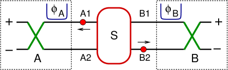
Figure 1: Schematic of the setup. A mesoscopic conductor acting as a source S (red box) is connected via four leads, $A1,A2,B1$ and $B2$, to regions A and B (dashed boxes), each containing two reservoirs, $+$ and $-$, a beamsplitter (green cross) and a sidegate (blue open box) which induces a phaseshift $\phi_{A}$ or $\phi_{B}$. Two particles (red dots) emitted from the source are shown.

A generic setup for such orbital QST is shown in Fig. 1. A mesoscopic conductor $S$ acts as a source for orbital quantum states. The source is connected via four single mode leads $A1,A2,B1$ and $B2$ to two regions, $A$ and $B$, where the emitted state is manipulated and detected. The mesoscopic source has one or more reservoirs biased at $eV$ and an arbitrary number of reservoirs kept at ground. We note that two-particles effects are only present for two or more reservoirs biased Buttnoise . The temperature is taken to be zero. It is assumed that the scattering in the conductor is elastic, however arbitrary debasing inside the conductor can be accounted for.

The regions $A$ and $B$ each contain an electronic beamsplitter BS1 ; BS2 and an electrostatic sidegate (see e.g. QHexp ) to induce a phaseshift, $\phi_{A}$ or $\phi_{B}$, by modifying the length of the lead. The beamsplitters, taken to be reflectionless, are further connected to two grounded reservoirs $+$ and $-$ where the current is measured. The combined beamsplitter-sidegate structure can be characterized by a scattering matrix, for e.g. $A$ given by

$$S_{A}=\left(\begin{array}[]{cc}\sqrt{R_{A}}e^{i\varphi_{A2}}&\sqrt{T_{A}}e^{i(\varphi_{A3}-\phi_{A})}\\ \sqrt{T_{A}}e^{i(\varphi_{A1}+\varphi_{A2})}&-\sqrt{R_{A}}e^{i(\varphi_{A1}+\varphi_{A3}-\phi_{A})\ }\end{array}\right).$$ (3)

The transmission probability $T_{A}=1-R_{A}$ can be controlled via electrostatic gating BS1 ; BS2 ; QHexp . The phases $\varphi_{Ai},~{}i=1,2,3$ picked up when scattering at the beamsplitter are however assumed to be uncontrollable but fixed during the measurement.

The quantum state emitted by the mesoscopic source is in the general case a manybody state, it is a linear superposition of states with different number of particles SSQI . However, one- and two-particle observables such as current and noise are only sensitive to the one- and two-particle properties of the state. These properties are quantified by the reduced density matrix, which thus is the object of interest. Only in some special cases, typically in conductors in the tunneling limit Orb ; QH1 ; QH2 , are the emitted states true one or two-particle states. In the presence of dephasing, the emitted state is mixed. Moreover, even an emitted pure manybody state generally gives rise to a mixed reduced one- or two particle state. It is therefore appropriate to discuss the state in terms of density matrices.

To simplify the discussion we consider a spin-polarized system with scattering amplitudes independent on energy on the scale of the applied bias $eV$, i.e. the linear voltage regime. The emitted state then has only orbital degrees of freedom. We first consider the single-particle orbital state emitted e.g. towards $A$ (same considerations hold for $B$). Introducing operators $b_{An}^{\dagger}$ creating electrons in lead $An$, with $n=1,2$, propagating out from the source, the $2\times 2$ density matrix (not normalized) is by definition given by

$$\rho_{A}=\sum_{n,m=1}^{2}\rho_{nm}b_{An}^{\dagger}|0\rangle\langle 0|b_{Am}=\left(\begin{array}[]{cc}\rho_{11}&\rho_{12}\\ \rho_{21}&\rho_{22}\end{array}\right)$$ (4)

where we work in the basis $\{|1\rangle_{A},|2\rangle_{A}\}$, with $b_{An}^{\dagger}|0\rangle=|n\rangle_{A}$, formed by the lead indices (see Fig. 1). The matrix elements $\rho_{nm}=\langle b_{Am}^{\dagger}b_{An}\rangle$. The Hermitian density matrix, $\rho_{A}=\rho_{A}^{\dagger}$, has four independent parameters and can be written as follows

$$\rho_{A}=\frac{1}{2}\sum_{i=0}^{3}c_{i}\sigma_{i}=\frac{1}{2}\left(\begin{array}[]{cc}c_{0}+c_{3}&c_{1}-ic_{2}\\ c_{1}+ic_{2}&c_{0}-c_{3}\end{array}\right),$$ (5)

where $\{\sigma_{i}\}=[{\bf 1},\sigma_{x},\sigma_{y},\sigma_{z}]$. A normalized density matrix is obtained by dividing all elements by $c_{0}$. In the same way, the two-particle density matrix is given by

$$\rho_{AB}=\sum_{n,m,k,l=1}^{2}\rho_{nm}^{kl}b_{An}^{\dagger}b_{Bk}^{\dagger}|0\rangle\langle 0|b_{Bl}b_{Am}$$ (6)

with the matrix elements $\rho_{nm}^{kl}=\langle b_{Am}^{\dagger}b_{Bl}^{\dagger}b_{Bk}b_{An}\rangle$. The two-particle density matrix has 16 independent parameters and can be written

$$\rho_{AB}=\frac{1}{4}\sum_{i,j=0}^{3}c_{ij}\sigma_{i}\otimes\sigma_{j}$$ (7)

with $\otimes$ the direct product. Expressing the real coefficients $c_{i}$ and $c_{ij}$ in terms of outcomes of ensemble averaged measurements thus gives a complete reconstruction of the emitted state. The accessible measurements are average current and zero frequency current correlations. Importantly, in the transport state the source continuously emits quantum states. As a consequence, the long time measurements automatically provide an ensemble average measurement. At $A$ the average currents at contacts $\alpha=\pm$ are

$$I_{A}^{\alpha}=\frac{e^{2}V}{h}\langle n_{A}^{\alpha}\rangle,\hskip 14.22636ptn_{A}^{\alpha}=b_{A\alpha}^{\dagger}b_{A\alpha}.$$ (8)

The zero frequency correlator between currents fluctuations $\Delta I$ in reservoirs $A\alpha$ and $B\beta$, given by $S_{AB}^{\alpha\beta}=(1/2)\int dt\langle\Delta I_{A\alpha}(0)\Delta I_{B\beta}(t)+\Delta I_{B\beta}(t)\Delta I_{A\alpha}(0)\rangle$ can be written Buttnoise

$$S_{AB}^{\alpha\beta} = \frac{2e^{3}V}{h}\left[\langle n_{A}^{\alpha}n_{B}^{\beta}\rangle-\langle n_{A}^{\alpha}\rangle\langle n_{B}^{\beta}\rangle\right]$$ (9)

with $n_{B}^{\alpha}=b_{B\alpha}^{\dagger}b_{B\alpha}$. The operators $b_{A\alpha}$ and $b_{B\beta}$ in the reservoirs at $A$ and $B$ are related to operators $b_{An}$ and $b_{Bk}$ in the leads $An,Bk$, with $n,k=1,2$, (see Fig. 1) via the scattering matrix $S_{A}$ of the beamsplitters at $A$ as

$$\left(\begin{array}[]{c}b_{A+}\\ b_{A-}\end{array}\right)=S_{A}\left(\begin{array}[]{c}b_{A1}\\ b_{A2}\end{array}\right)$$ (14)

and similarly at $B$.

We start with the reconstruction of the one-particle state at $A$, accessible via the average current (the same procedure holds for the state at $B$). Here a formal approach is taken which directly can be extended to the investigation of the two-particle state. We note that the reconstruction approach is similar to QST schemes for qubits in other systems, see e.g. Refs. Kwiat2 ; Nori . There are however a number of important special features for mesoscopic systems, making a detailed investigation important. It is desirable to minimize both the type and number of experiments having to be carried out. As is clear from the following, for a complete reconstruction it is sufficient to consider only measurements of currents in one reservoir in $A$. Here we consider the current at $A+$. Using the relation between operators, Eq. (14), and Eq. (8), we have

$$I_{A}^{+}/(e^{2}V/h)=\langle n_{A}^{+}\rangle=\mbox{tr}\left(\rho_{A}{\cal A}\right)$$ (15)

with the matrix

$${\cal A}=\left(\begin{array}[]{cc}R_{A}&\sqrt{T_{A}R_{A}}e^{-i(\phi_{A}+\varphi_{A})}\\ \sqrt{T_{A}R_{A}}e^{i(\phi_{A}+\varphi_{A})}&T_{A}\end{array}\right).$$ (18)

The phase $\varphi_{A}=\phi_{A2}-\phi_{A3}$ contains all the information about uncontrollable phases of the beamsplitter. From Eqs. (15) and (18) it is clear that the phase $\varphi_{A}$ can be included in $\rho_{A}$ by a change of local basis $\rho_{A}\rightarrow U_{A}\bar{\rho}_{A}U_{A}^{\dagger}$ with $U_{A}=\mbox{diag}[\mbox{exp}(-i\varphi_{A}/2),\mbox{exp}(i\varphi_{A}/2)]$. Below we consider the reconstruction of $\bar{\rho}_{A}$, parameterized by coefficients $\bar{c}_{i}$ [see Eq. (5)], thus working with ${\mathcal{A}}(\varphi_{A}=0)$ in Eq. (18). This yields $\rho_{A}$ up to an unknown local basis rotation.

Importantly, only four settings of the beamsplitter are needed, both for the current and the current correlators, for a complete state reconstruction. The settings $I$ to $IV$ considered here are listed in the table in Fig. 2.

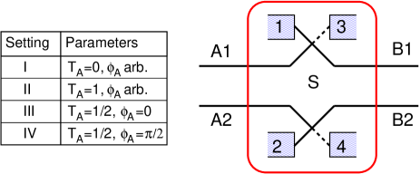
Figure 2: Left: Table with scattering parameters at $A$ for the four different settings. Right: Schematic of an elementary mesoscopic source S (red box, see Fig. 1). Two reservoirs biased at $eV$, $1$ and $2$, and two grounded reservoirs, $3$ and $4$ are connected via beamsplitters to the four leads going out towards $A$ and $B$. Scattering between upper and lower leads, e.g. $A1$ and $A2$, is not possible.

By constructing suitable linear combinations $j_{A}(j)$ of the observables at the different settings, in the $\{|1\rangle_{A},|2\rangle_{A}\}$ basis

$$j_{A}(0) = {\mathcal{A}}(I)+{\mathcal{A}}(II)={\bf 1},$$

$$j_{A}(1) = 2{\mathcal{A}}(III)-\left[{\mathcal{A}}(I)+{\mathcal{A}}(II)\right]=\sigma_{x},$$

$$j_{A}(2) = 2{\mathcal{A}}(IV)-\left[{\mathcal{A}}(I)+{\mathcal{A}}(II)\right]=\sigma_{y},$$

$$j_{A}(3) = {\mathcal{A}}(I)-{\mathcal{A}}(II)=\sigma_{z},$$ (19)

we obtain a complete set Fano of measurements, since the Pauli matrices $\sigma_{j}$ obey the relation $\mbox{tr}(\sigma_{i}\sigma_{j})=2\delta_{ij}$. Here ${\mathcal{A}(I)}$ is the matrix ${\mathcal{A}}$ in Eq. (18) for the setting I etc. From Eqs. (15) and (19) and the relation $\langle j_{A}(j)\rangle=\mbox{tr}(\bar{\rho}_{A}\sigma_{j}\rangle=\bar{c}_{j}$ we then directly obtain the coefficients $\bar{c}_{j}$, parametrizing $\rho_{A}$ in Eq. (5)

$$\bar{c}_{j} = \sum_{k=0}^{3}Q_{jk}\langle n_{A}^{+}(k)\rangle,\hskip 2.84544ptQ=\left(\begin{array}[]{cccc}1&1&0&0\\ -1&-1&2&0\\ -1&-1&0&2\\ 1&-1&0&0\end{array}\right)$$ (24)

in terms of the measured currents for the different settings, taking the index $\{k\}=[0,1,2,3]\equiv[I,II,II,IV]$. This completes the one-particle state reconstruction.

We then turn to the two-particle state. In Eq. (9), the quantity that is directly linked to the density matrix elements $\rho_{nm}^{kl}$ is the reducible correlator $\langle n_{A}^{\alpha}n_{B}^{\beta}\rangle$. This correlator is directly obtained from the measured noise and the average currents. In analogy to the current, it is sufficient to consider correlations between currents in one terminal in $A$ and one in $B$. Considering here $A+$ and $B+$, one obtains from Eq. (9) and (14) the dimensionless correlator

$$\frac{S_{AB}^{++}}{2e^{3}V/h}+\frac{I_{A}^{+}I_{B}^{+}}{(e^{2}V/h)^{2}}=\langle n_{A}^{+}n_{B}^{+}\rangle=\mbox{tr}\left(\rho_{AB}{\cal A}\otimes{\cal B}\right)$$ (25)

where the matrix ${\cal B}$ is given from ${\cal A}$ in Eq. (18) by changing indices $A\rightarrow B$ in the scattering amplitudes. Similar to the one-particle state, we note from Eq. (25) that both phases $\varphi_{A}$ and $\varphi_{B}$ can be included in $\rho_{AB}$ by independent local rotations $\rho_{AB}\rightarrow(U_{A}\otimes U_{B})\bar{\rho}_{AB}(U_{A}\otimes U_{B})^{\dagger}$, with $U_{B}=\mbox{diag}[\mbox{exp}(-i\varphi_{B}/2),\mbox{exp}(i\varphi_{B}/2)]$. Below we thus consider the reconstruction of $\bar{\rho}_{AB}$, parameterized as in Eq. (7) by the coefficients $\bar{c}_{ij}$, yielding $\rho_{AB}$ up to a local basis rotation entcom .

By considering the same four settings at $B$ as at $A$, we can use the linear combination operators $j_{A}(j)$ in Eq. (19) and correspondingly $j_{B}(i)$ to construct a complete set of observables, in the basis $\{|1\rangle_{A}|1\rangle_{B},|1\rangle_{A}|2\rangle_{B},|2\rangle_{A}|1\rangle_{B},|2\rangle_{A}|2\rangle_{B}\}$,

$$j_{A}(j)j_{B}(i)=\sigma_{j}\otimes\sigma_{i}$$ (26)

since the direct products of $\sigma$-matrices obey $\mbox{tr}\left[(\sigma_{j}\otimes\sigma_{i})(\sigma_{k}\otimes\sigma_{l})\right]=4\delta_{jk}\delta_{il}$. From Eq. (25) and the relation $\langle j_{A}(j)j_{B}(i)\rangle=\mbox{tr}(\bar{\rho}_{AB}\sigma_{j}\otimes\sigma_{i}\rangle=\bar{c}_{ji}$ we then directly obtain the coefficients $\bar{c}_{ji}$ as

$$\bar{c}_{ji}=\sum_{k,l=0}^{3}Q_{jk}Q_{il}\langle n_{A}^{+}(k)n_{B}^{+}(l)\rangle$$ (27)

in terms of the measured current correlators and averaged currents. We emphasize that all elements can be determined from sixteen current correlations and eight average currents (four at $A$ and four at $B$). We also note that the reconstructed density matrix, due to nonideal measurements, might have negative eigenvalues, i.e. it might not be positive semidefinite. Schemes to correct for this for one and two-qubit states are discussed in e.g. ref. Kwiat2 .

In the context of two-particle entanglement, it is interesting to compare the QST-scheme with a Bell Inequality, recently discussed for mesoscopic system (see e.g. refs. Cht ; Orb and for a density matrix approach ref. Carlodeph ). Both schemes require the same number of current correlation measurements. The density matrix reconstructed by QST however completely determines the entanglement. In contrast, a Bell Inequality can not be used to quantify the entanglement Verstraete , there are e.g. mixed entangled states Werner that do not lead to a violation of a Bell Inequality.

It is clarifying to illustrate the above scheme with a simple example (see Fig. 2). We consider the Hanbury Brown Twiss geometry of ref. QH2 , where the number of nonzero elements of the one and two-particle density matrices are reduced due to the topological properties of the conductor. Since no scattering between the upper, $1$, and lower, $2$, leads is physically possible due to the spatial separation, the one-particle density matrix $\bar{\rho}_{A}$ only has two nonzero elements, $\bar{\rho}_{11}$ and $\bar{\rho}_{22}$. These elements are parametrized by $\bar{c}_{0}$ and $\bar{c}_{3}$, obtained by measuring $\langle j_{A}(0)\rangle$ and $\langle j_{A}(3)\rangle$.

The two-particle density matrix $\bar{\rho}_{AB}$ has four nonzero elements, $\bar{\rho}_{11}^{22},\bar{\rho}_{22}^{11},\bar{\rho}_{21}^{12}$ and $\bar{\rho}^{21}_{12}$. Using the relation between the coefficients $\bar{c}_{ij}$ resulting from several matrix elements being zero, $\bar{\rho}_{AB}$ can then be parameterized as

$$\bar{\rho}_{AB}=\frac{1}{2}\left(\begin{array}[]{cccc}0&0&0&0\\ 0&\bar{c}_{00}+\bar{c}_{33}&\bar{c}_{11}-i\bar{c}_{21}&0\\ 0&\bar{c}_{11}+i\bar{c}_{21}&\bar{c}_{00}-\bar{c}_{33}&0\\ 0&0&0&0\end{array}\right).$$ (28)

Conseqently, only four correlations $\langle j_{A}(i)j_{B}(j)\rangle$ need to be measured to completely reconstruct $\bar{\rho}_{AB}$, reducing the number of actual current correlations needed to be carried out to 12 for the settings considered here [see Eq. (27)]. It is interesting to note that in the geometry in Fig. 2, considering the tunneling limit for the beamsplitters in the source and changing to an electron-hole picture QH1 , the emitted state is a true two-particle state QH2 . Since the hole currents and current fluctuations are directly related to the electron ones, it is possible to employ our scheme to reconstruct an electron-hole state as well.

In conclusion, we have presented a scheme for orbital Quantum State Tomography, a complete reconstruction of orbital quantum states in mesoscopic conductors in the transport state. The emitted orbital states are manipulated with electronic beamsplitters and detected with currents and zero frequency current correlations. With all components experimentally available, our scheme opens up for a direct observation of quasiparticle quantum states in mesoscopic conductors.

We acknowledge discussions with E.V. Sukhorukov. This work was supported by the Swedish Research Council, the Swiss National Science Foundation and the program for Materials with Novel Electronic Properties.

References

- (1) Historically, W. Pauli, General Principles of Quantum Mechanics (Springer, Berlin, 1980) addressed the problem for position and momentum measurements in 1933.
- (2) U. Fano, Rev. Mod. Phys. 29, 74 (1957).
- (3) J. Bertrand and P. Bertrand, Found. Phys. 17, 397 (1987); K. Vogel and H. Risken, Phys. Rev. A 40, 2847 (1989); A. Royer, Found. Phys. 19, 3 (1989); U. Leonhardt, Phys. Rev. B 53, 2998 (1996); M. G. Raymer, Cont. Phys. 38, 343 (1997).
- (4) J.R. Ashburn et al, Phys. Rev. A 41, 2407 (1990).
- (5) D.T. Smithey et al, Phys. Rev. Lett. 70, 1244 (1993).
- (6) T.J. Dunn, I.A. Walmsey and S. Mukamel, Phys. Rev. Lett. 74, 884 (1995).
- (7) D. Liebfried et al, Phys. Rev. Lett. 77, 4281 (1996).
- (8) Ch. Kurtsiefer, T. Pfau, and Mlynek, Nature 386, 150 (1997).
- (9) P.G. Kwiat et al, Nature 409 1014 (2001); T. Yamamoto et al, ibid 421, 343 (2003).
- (10) Y. Liu, L.F. Wei, and F. Nori, Europhys. Lett. 67, 187 (2004); quant-ph/0407197.
- (11) P. Samuelsson, E.V. Sukhorukov, and M. Büttiker, Phys. Rev. Lett. 91, 157002 (2003).
- (12) C.W.J. Beenakker et al, Phys. Rev. Lett. 91, 147901 (2003).
- (13) P. Samuelsson, E.V. Sukhorukov, and M. Büttiker, Phys. Rev. Lett. 92, 026805 (2004).
- (14) M. Henny et al., Science 284, 296 (1999); S. Oberholzer et al., Physica 6E, 314 (2000).
- (15) W.D. Oliver et al., Science 284, 299 (1999).
- (16) M. Büttiker, Phys. Rev. B 46, 12485 (1992).
- (17) Ya. Blanter and M. Büttiker, Phys. Rep. 336, 1 (2000).
- (18) Y. Ji et al., Nature 422, 415 (2003).
- (19) G. Burkhard, D. Loss, and E.V. Sukhorukov, Phys. Rev. B 61, 16303 (2000).
- (20) N. Chtchelkatchev et al, Phys. Rev. B 66, 161320 (2002).
- (21) See e.g. P. Samuelsson, E.V. Sukhorukov, and M. Büttiker, cond-mat/0503016 for a recent discussion.
- (22) D. James et al, Phys. Rev. A 64, 052312 (2001).
- (23) Note that e.g. the entanglement is invariant under such a local rotation .
- (24) J.L. van Velsen et al, Turk. J. Phys. 27, 323 (2003).
- (25) F. Verstraete and M. Wolf, Phys. Rev. Lett. 89, 170401 (2002).
- (26) R.F. Werner, Phys. Rev. A 40, 4277 (1989).