Configurational entropy of hard spheres

Abstract

We numerically calculate the configurational entropy $S_{conf}$ of a binary mixture of hard spheres, by using a perturbed Hamiltonian method trapping the system inside a given state, which requires less assumptions than the previous methods [R.J. Speedy, Mol. Phys. 95, 169 (1998)]. We find that $S_{conf}$ is a decreasing function of packing fraction $\varphi$ and extrapolates to zero at the Kauzmann packing fraction $\varphi_{{}_{K}}\simeq 0.62$, suggesting the possibility of an ideal glass-transition for hard spheres system. Finally, the Adam-Gibbs relation is found to hold.

1 Introduction

The idea that the glass transition is driven by a decreasing of the number of accessible states upon lowering temperature (or raising density) is quite old [1, 2, 3]. In this picture, if crystallization is avoided, an ideal glass transition is expected to happen at the point where the configurational entropy $S_{conf}$ (the logarithm of the number of states) vanishes. When the liquid enters in the the supercooled region, the dynamics becomes slower and slower and the particles get trapped for an increasingly longer time inside the “cages” made by their neighbors: the dynamics of the system can be successfully described as a “fast” motion of the representative point in the $3N$ configuration space inside metastable states, and a “slow” motion corresponding to jumps among states. Entering more in the supercooled region the number of accessible metastable states decreases and the extrapolation to zero of $S_{conf}$ defines the ideal glass transition. In experiments (or numerical simulations) the region close to the ideal glass transition is unreachable, due to the “apparent” arrest of the system at the so called glass-transition temperature (or density) when relaxation times become longer than experimental time scale. The above scenario has been shown to be valid for many interacting systems, based on smooth pair-potential (as Lennard-Jones liquids), for which the Potential Energy Landscape (PEL) approach [4, 5, 6, 7, 8, 9, 10, 11, 12, 13] and the replica method [14, 15] have allowed to give numerical estimations of $S_{conf}$ and of the ideal glass transition.

The overall picture is still not well established for Hard Spheres (HS), for which the existence of a glass transition is still an open question [16, 17, 18, 19, 20]. A particularly important role seems to be played by the dimesionality of the system. In particular in d=2 dimension there are numerical [20, 21] and theoretical [22, 23] evidences of the absence of a thermodynamic glass transition, while the opposite seems to be true in d=3 [18, 24]. Moreover, the step-wise form of the interparticle potential does not allow a PEL analysis and different approaches have to be taken in consideration in order to calculate the configurational entropy $S_{conf}$. In the past, attempts to estimate $S_{conf}$ have been performed based on different evaluations of the entropy in each single state [18, 25, 26]. Recently the replica method has been extended to the HS case for one-component systems [23, 24].

In this paper we follow an approach, based on the Frenkel-Ladd method [27] and recently introduced in the study of Lennard-Jones systems [28] and attractive colloids [29, 30], to numerically estimate $S_{conf}$ for binary hard spheres. As in previous studies, the calculation is reduced to that of vibrational entropy $S_{vib}$, using the fact that the total entropy $S$ can be decomposed into the sum of a configurational contribution $S_{conf}$ and a vibrational one $S_{vib}$:

$$S=S_{conf}+S_{vib}\ .$$ (1)

This expression is consistent with the idea that, at high enough density, there are two well separated time scales: a fast one, related to the motion inside a local state (the rattling in the cage), and a slow one associated to the exploration of different states.
The total entropy $S$ is obtained by thermodynamic integration, starting from the ideal gas state. The quantity $S_{vib}$ is calculated using a perturbed Hamiltonian, adding to the original Hamiltonian an harmonic potential around a given reference configuration. Calculating the mean square displacement from the reference configuration and making an integration over the strength of the perturbation, it is possible to estimate the vibrational entropy [29]. The difference $S-S_{vib}$ provides an estimate of the configurational entropy $S_{conf}$ as a function of packing fraction $\varphi$ (or density $\rho$).

The main findings of the present work are the following. i) $S_{conf}$ is a decreasing function of packing fraction $\varphi$, and a suitable extrapolation to zero provides and estimate of the ideal phase transition point (Kauzmann packing fraction) $\varphi_{{}_{K}}\simeq 0.62$. ii) The diffusivity $D$ and configurational entropy $S_{conf}$ are related through the Adam-Gibbs relation, in agreement with previous claims [18].

2 The model

The studied system is a binary mixture $50-50$ of hard spheres, $A$ and $B$, with diameters ratio $\sigma_{{}_{B}}/\sigma_{{}_{A}}$=$1.2$. The collision diameters are $\sigma_{{}_{AA}}$=$\sigma_{{}_{A}}$, $\sigma_{{}_{BB}}$=$\sigma_{{}_{B}}$ and $\sigma_{{}_{AB}}$=$(\sigma_{{}_{A}}+\sigma_{{}_{B}})/2$. The particles ($N$=$256$) are enclosed in a cubic box with periodic boundary conditions. We use the following units: $\sigma_{{}_{B}}$ for length and $m_{A}=m_{B}=1$ for mass. Moreover we chose $k_{B}=1$ and $\hbar=1$. The density is measured by the packing fraction $\varphi$ that is related to the number density $\rho=N/V$ by $\varphi$=$\rho\pi(\sigma_{{}_{A}}^{3}+\sigma_{{}_{B}}^{3})/12$. We analyzed systems in the range $\varphi$=$0.425-0.580$. Hard spheres systems depend only trivially on temperature that sets an overall scale for the dynamics, consequently we perform all our simulations at $T=1$. We performed standard event-driven molecular dynamics [31] and we stored several equilibrated configurations at different density.

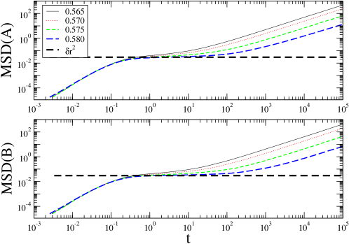
Figure 1: Mean square displacements (MSD) of the species $A$ (top) and $B$ (bottom). Both MSDs has been normalized by the value of the diameter squared. The dashed lines represent the cage size squared, $\delta r^{2}$.

3 Diffusivity

The diffusion coefficients $D$ of the two species have been extracted from the long time limit of the mean square displacements (MSD) $\langle r^{2}(t)\rangle$=$N^{-1}\langle[{\bf r}(t)-{\bf r}(0)]^{2}\rangle$ (${\bf r}$ is the $3N$-vector of the coordinates):

$$\lim_{t\rightarrow\infty}\frac{\langle r^{2}(t)\rangle}{t}\simeq 6D\ .$$ (2)

To improve the statistical significance of the data, an average over $10$ independent runs have been performed. In Fig 1 the mean squared displacements for the slowest cases, i.e. $\phi>0.56$, are presented for both species. It is clear that on increasing the density the MSDs develop the typical two step relaxation pattern. The first part of the MSD is purely ballistic while, at later stage, it reaches the diffusive regime, described by Eq. 2. Between this two regimes a plateau starts to develop. This is the clear indication of a caging effect. Each particle starts to feel the crowding of its neighbors and it is trapped in a cage for longer and longer time on increasing the density. The height of the plateau is the typical “cage diameter squared”, $\delta r^{2}$. For both species we find $\delta r^{2}=3\cdot 10^{-2}\sigma_{\alpha}^{2}$ for $\alpha=A\mbox{ or }B$ represented by a dashed line in Fig. 1. This is a clear evidence that the two species have the same caging effect. We shall return on the value of $\delta r^{2}$ later on.

In Fig. 2 the diffusivities $D$ of A and B particles are plotted as a function of the packing fraction $\varphi$. Dashed lines in the figure are power-law fits $D=C\;(\varphi_{c}-\varphi)^{\gamma}$ of the high packing-fraction data ($\varphi\geq 0.53$), as predicted by mode-coupling theory. The fitted parameters are: $\varphi_{c}$=$0.583$, $\gamma$=$2.27$, $C$=$9.50$ for A particles and $\varphi_{c}$=$0.583$, $\gamma$=$2.47$, $C$=$11.66$ for B particles. We note that both diffusivities give rise to the same mode-coupling packing fraction $\varphi_{c}$, in agreement with the prediction of the theory [32] and with previous simulations of the same model [33].

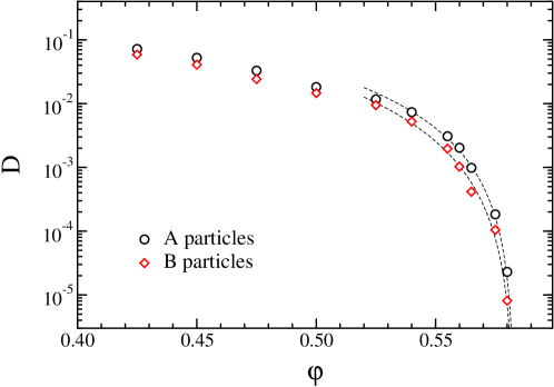
Figure 2: Diffusivity for A and B particles as a function of packing fraction $\varphi$. The lines are power-law fits for $\varphi\geq 0.53$, $C\;(\varphi_{c}-\varphi)^{\gamma}$, with: $\varphi_{c}$=$0.583$, $\gamma$=$2.27$, $C$=$9.50$ for A particles; $\varphi_{c}$=$0.583$, $\gamma$=$2.47$, $C$=$11.66$ for B particles.

4 Configurational entropy

We now turn to the calculation of configurational entropy. The method we follow to estimate $S_{conf}$ requires the computation of the total entropy $S$ and vibrational entropy $S_{vib}$. The total entropy $S$ is calculated via a thermodynamic integration from ideal gas and can be expressed as

$$S(\rho)=S_{id}(\rho)+S_{ex}(\rho)\ ,$$ (3)

where $S_{id}$ is the entropy of the ideal gas and $S_{ex}$ is the excess entropy with respect to the ideal gas. For a binary mixture, the ideal gas entropy is:

$$\frac{S_{id}(\rho)}{N}=\frac{5}{2}-\ln{\rho}-3\ln{\lambda}+\ln{2}\ ,$$ (4)

where $\lambda=(2\pi\beta\hbar^{2}/m)^{\frac{1}{2}}$ is the De Broglie wavelength ($\hbar$ is the Planck’s constant and has been set to unitary value), and the term $\ln{2}$ takes into account the mixing contribution. The term $S_{ex}$ can be expressed in the following form

$$S_{ex}(\rho)=-\frac{N}{T}\int_{0}^{\rho}\frac{d\rho}{\rho^{2}}\ P_{ex}\ ,$$ (5)

with $P_{ex}$ the excess pressure. We extracted $P_{ex}$ from the zero density limit up to the densities of interest, performing numerical simulations and fitting the results of the pressure with a high order polynomial in $\rho$. In Fig. 3 we show the numerically calculated excess entropy $S_{ex}$ (symbols) together with the analytic estimate provided by the Carnahan-Starling (CS) equation of state, extended to hard sphere mixtures [34, 35, 36]. We note that at high densities the CS equation of state overestimates the entropy of about $7\%$. This discrepancy, however, is not sufficiently significant to affect the resulting $S_{conf}$ values, in particularly closed to the glass transition.

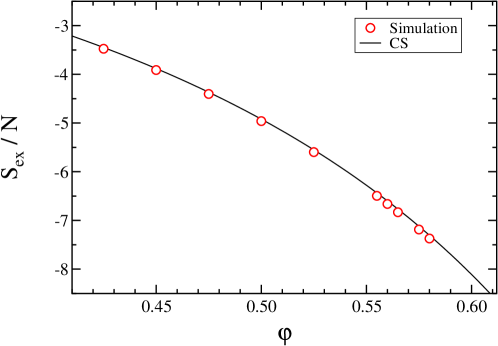
Figure 3: Excess entropy $S_{ex}$ for the mixture of hard spheres as obtained from our simulations (symbols) compared with the analytical Carnahan-Starling expression (line) [35, 36].

The method we use for the calculation of $S_{vib}$ is based on the investigation of a perturbed system

$$\beta H^{\prime}=\beta H+\alpha N({\bf r}-{\bf r}_{0})^{2}\ ,$$ (6)

where $H$ is the unperturbed hard spheres Hamiltonian, $\alpha$ is the strength of the perturbation, ${\bf r}_{0}$ specifies the particles coordinates of a reference configuration and $({\bf r}-{\bf r}_{0})^{2}\equiv N^{-1}\sum_{i=1}^{N}({\vec{r}}_{i}-{\vec{r}}_{0,i})^{2}$. The reference configuration ${\bf r}_{0}$ is chosen from equilibrium configurations at the considered density (randomly extracted from the stored configurations obtained during molecular dynamics simulations). With this choice one is sure that the estimated vibrational entropy (see formula below) pertains to the correct state at the studied density. The vibrational entropy can be obtained from the formula (see Ref. [29] for details):

$$\frac{S_{vib}}{N}=\int_{\alpha_{0}}^{\alpha_{\infty}}d\alpha^{\prime}\langle({\bf r}-{\bf r}_{0})^{2}\rangle_{\alpha^{\prime}}-\frac{3}{2}\ln\left(\frac{\alpha_{\infty}\lambda^{2}}{\pi}\right)+\frac{3}{2}\ ,$$ (7)

where $\alpha_{0,\infty}$ are the lower/upper limit of integration, and $\langle...\rangle_{\alpha^{\prime}}$ is the canonical average for a given $\alpha^{\prime}$. The choice of $\alpha_{0}$ deserves few comments. If the system were confined to move inside a given local free-energy minimum, for a correct estimation of $S_{vib}$ one would take the lower limit $\alpha_{0}$=$0$ in the integral in Eq. 7. As the system, at enough low value of $\alpha$, begins to sample different states (the harmonic force due to the perturbation is no more able to constrain the system inside one state), $\alpha_{0}$ has to be chosen in such a way that the system has not yet left the state: the underlying idea is that Eq. 7 gives a correct estimation of $S_{vib}$ until the system remains trapped in the state. An appropriate choice in our case seems to be $\alpha_{0}^{(1)}$=$2^{2.5}$ for all the densities , as, close to this point, one observes a crossover for all the investigated densities (more pronounced for low density data). In Fig. 4 the quantity $\langle({\bf r}-{\bf r}_{0})^{2}\rangle_{\alpha}$ is reported as a function of $\alpha$. An arrow indicates the chosen value $\alpha_{0}$=$\alpha_{0}^{(1)}$, below which one observes the crossover associated to the exploration of different states.

It is worth noting that different choices of $\alpha_{0}$ are in principle possible, giving rise to different estimations of the vibrational entropy term. However, even though a kind of arbitrariness is present in the method, one can argue that a reasonable choice should be for values above $\alpha_{0}^{(1)}$ (close to the crossover corresponding to the exploration of different states) and below an upper value $\alpha_{0}^{(2)}$ at which one is sure that the system is still confined in a single state. The latter value can be estimated requiring that the MSD $\langle({\bf r}-{\bf r}_{0})^{2}\rangle$ is always close/below the cage diameter squared $\delta r^{2}\simeq 3\cdot 10^{-2}\sigma_{\alpha}^{2}$ (with $\alpha=A\mbox{ or }B$) (this has been estimated from the plateau of the mean square displacement, see Fig. 1).

The chosen value in our case is $\alpha_{0}^{(2)}$=$2^{4.5}$ (indicated by an arrow in Fig. 4). We then repeated the same calculation of $S_{vib}$ using Eq.7 with the lower bound in the integral $\alpha_{0}=\alpha_{0}^{(2)}$. In this way we obtain a lower and upper bound for the quantity of interest $S_{vib}$, by using respectively $\alpha_{0}^{(1)}$ or $\alpha_{0}^{(2)}$ in the expression of $S_{vib}$ in Eq.7.

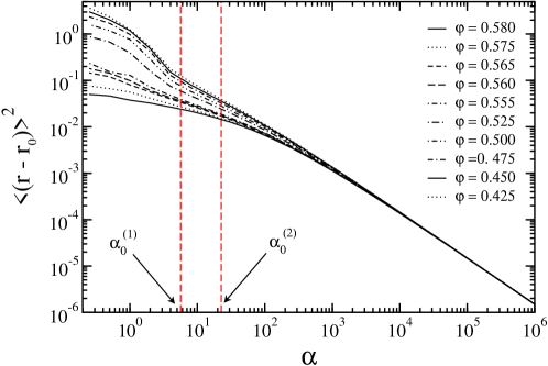
Figure 4: The quantity $\langle({\bf r}-{\bf r}_{0})^{2}\rangle_{\alpha}$ plotted vs. $\alpha$ in logarithmic scale for different packing fractions $\varphi$. Vertical lines are the values $\alpha_{0}^{(1)}=2^{2.5}$ and $\alpha_{0}^{(2)}=2^{4.5}$ used as $\alpha_{0}$-value in the integral in Eq. 7 for the calculation of $S_{vib}$.

Fig. 5 shows $S_{conf}$ as a function of $\varphi$. The configurational entropy $S_{conf}$ is calculated using Eq. 1, where the two entropies $S$ and $S_{vib}$ are obtained from Eq.s 3 and 7 respectively. Due to the fact that the correct integral for the estimation of $S_{vib}$ should be done from $\alpha_{0}$=$0$, but with the system always inside a given state, we have added to the expression in Eq. 7 the term $\alpha_{0}\;\langle({\bf r}-{\bf r}_{0})^{2}\rangle_{\alpha_{0}}$, corresponding to assume a constant value of $\langle({\bf r}-{\bf r}_{0})^{2}\rangle$ below $\alpha_{0}$ and using a zero value for the lower limit of the integral in Eq. 7. Fig. 5 shows the two estimates of $S_{conf}$, corresponding to the two different values of $\alpha_{0}$: $\alpha_{0}^{(1)}$=$2^{2.5}$ (open symbols) and $\alpha_{0}^{(2)}$=$2^{4.5}$ (full symbols). One observes that the discrepancy between the two estimations decreases by increasing the packing fraction, suggesting that, at high density, the method used to calculate $S_{conf}$ is less affected by the choice of the free parameters entering in its evaluation. This is probably due to the fact that increasing the density the system tends to be more trapped in a local free-energy minimum. Indeed, it is only at high density that the method is expected to work better, due to the better definition of two time scales corresponding to local-fast and global-slow dynamics (see Fig. 1). At low density, instead, the two are less separated and this corresponds to a difficulty in the extrapolation for $\alpha_{0}\to 0$ of the quantity reported in Fig. 4. The low density data show a more clear crossover on lowering $\alpha$, and then a worst definition of state in this limit. As we are interested in the high packing fraction extrapolation, this fact do not affect our prediction on the Kauzmann density value.

Figure 5: Configurational entropy $S_{conf}$ as function of packing fraction $\varphi$. Open symbols are data using $\alpha_{0}^{(1)}=2^{2.5}$, full symbols using $\alpha_{0}^{(2)}=2^{4.5}$ (see text). Dashed and dot-dashed lines are from Speedy [18] for binary and monatomic hard-spheres respectively. Thin full line is the analytical computation of Parisi and Zamponi for monatomic hard-spheres [24]. Thick lines are polynomial extrapolations of our data in the high packing fraction region, giving rise to the same Kauzmann packing fraction estimation for which $S_{conf}(\varphi_{K})$=$0$: $\varphi_{{}_{K}}\simeq 0.62$.

Also reported in the figure are the curves obtained by Speedy [18] using a different method (assuming a particular form of the vibrational entropy, a Gaussian distribution of states and involving some free parameters) for the estimation of $S_{conf}$, for monatomic (dot-dashed line) and binary (dashed line) hard-spheres (with the same diameters ratio $1.2$ and composition $50:50$ as in our case). It is worth noting that our method improves on Speedy’s one, as, even though requiring some accuracy in the choice of the $\alpha_{0}$ parameter, has the advantage to be less affected by the presence of many free parameters and particular assumptions. We note that the data of Speedy for the binary case do agree very well with our data with $\alpha_{0}$=$\alpha_{0}^{(2)}$, suggesting the possibility that the choice of $\alpha_{0}$=$\alpha_{0}^{(2)}$ is more accurate for the estimation of $S_{vib}$ and so of $S_{conf}$. As a comparison, in Fig. 5 is also reported an analytic estimation of $S_{conf}$ recently provided by Parisi and Zamponi [24] for monatomic hard-spheres. From the $\varphi$-dependence of the configurational entropy one can determine the packing fraction at which $S_{conf}$ extrapolates to zero, corresponding to the ideal phase transition point (Kauzmann packing fraction $\varphi_{{}_{K}}$) $S_{conf}(\varphi_{{}_{K}})$=$0$. Using a polynomial extrapolation [37] for the two set of data (corresponding to the different $\alpha_{0}$ values) we obtain an estimated Kauzmann packing fraction value $\varphi_{{}_{K}}\simeq 0.62$ (see Fig.5). It is worth noting that, even though the two curves are quite different, the estimated value of $\varphi_{{}_{K}}$ is the same, again suggesting the robustness of the method in the high density region and then in the estimation of the Kauzmann packing fraction.

5 Adam-Gibbs relation

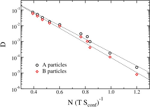
Figure 6: The Adam-Gibbs relation $D$=$D_{\infty}\exp[-N\Delta/(TS_{conf})]$ ($T$=$1$) for the two species A and B: $D_{\infty}$=$3.66$, $\Delta$=$9.8$ for A particles; $D_{\infty}$=$4.59$, $\Delta$=$10.5$ for B particles. The data of $S_{conf}$ are obtained with $\alpha_{0}$=$\alpha_{0}^{(2)}$.

In this Section we explore the validity of the Adam-Gibbs relation, linking dynamic quantities, like diffusivity, to $S_{conf}$. In Fig. 6 we report the diffusivities $D$ for A and B particles vs. the quantity $(TS_{conf})^{-1}$, with $S_{conf}$ obtained for the value $\alpha_{0}$=$\alpha_{0}^{(2)}$. We find that the Adam-Gibbs relation

$$D=D_{\infty}e^{-N\Delta/TS_{conf}}$$ (8)

is verified (lines in the figure), with: $D_{\infty}$=$3.66$, $\Delta$=$9.8$ for A particles; $D_{\infty}$=$4.59$, $\Delta$=$10.8$ for B particles. A similar behavior is obtained using $S_{conf}$ calculated with $\alpha_{0}$=$\alpha_{0}^{(1)}$ (not shown in the figure), with the values: $D_{\infty}$=$24.5$, $\Delta$=$9.5$ for A particles; $D_{\infty}$=$37.5$, $\Delta$=$10.5$ for B particles, suggesting that, in this range of diffusivity values, the AG expression is not able to discriminate between the two different estimations of $S_{conf}$.

6 Conclusions

In conclusion, we have calculated $S_{conf}$ for binary mixture hard spheres, by numerically estimating the total entropy $S$ (via thermodynamic integration from ideal gas) and the vibrational entropy $S_{vib}$ using a numerical procedure based on Frenkel-Ladd method and recently applied in the analysis of Lennard-Jones systems and attractive colloids: the system is constrained inside a given “state” through an harmonic perturbed term in the Hamiltonian. We found, in agreement with analytical and simulation results in the literature, that $S_{conf}$ is a decreasing function of the packing fraction $\varphi$, suggesting the possibility of a vanishing of $S_{conf}$ around the Kauzmann point $\varphi_{{}_{K}}$=$0.62$. Moreover, by studying the relationship between $S_{conf}$ and the diffusion constant $D$, the Adam-Gibbs relation is found to reasonably hold for the analyzed system.

References

References

- [1] Kauzmann A W 1948 Chem. Rev. 43 219
- [2] Adam G and Gibbs J H 1958 J. Chem. Phys. 43 139
- [3] Gibbs J H and Di Marzio E A 1958 J. Chem. Phys. 28 373
- [4] Debenedetti P G and Stillinger F H 2001 Nature 410 259
- [5] Stillinger F H and Weber T A 1984 Science 225 983
- [6] Stillinger F H 1995 Science 267 1935
- [7] Sciortino F, Kob W and Tartaglia P 1999 Phys. Rev. Lett. 83 3214
- [8] Scala A, Starr F W, La Nave E, Sciortino F and Stanley H E 2000 Nature 406 166
- [9] Sastry S, Debenedetti P G and Stillinger F H 1998 Nature 393 554
- [10] Büchner S and Heuer A 2000 Phys. Rev. Lett. 84 2168
- [11] Sastry S 2001 Nature 409 164
- [12] Keyes T 1997 J. Phys. Chem. 101 2921
- [13] Sciortino F 2005 J. Stat. Mech. P05015
- [14] Mézard M and Parisi G 1999 J. Chem. Phys. 111 1076
- [15] Coluzzi B , Parisi G and Verrocchio P 2000 J. Chem. Phys. 112 2933
-
[16]
Rintoul M D and Torquato S 1996
Phys. Rev. Lett. 77 4198
Rintoul M D and Torquato S 1996 J. Chem. Phys. 105 9258 - [17] Robles M, Lòpez de Haro M, Santos A and Bravo Yuste S 1998 J. Chem. Phys. 108 1290
- [18] Speedy R J 1998 Mol. Phys. 95 169
- [19] Tarzia M, de Candia A, Fierro A, Nicodemi M and Coniglio A 2004 Europhys. Lett. 66 531
- [20] Donev A, Stillinger F H and Torquato S 2006 Phys. Rev. Lett. 96 225502
- [21] Santen L and Krauth W 2000 Nature 405 550
- [22] Tarzia M 2007 J. Stat. Mech. P01010
- [23] Zamponi F 2006 Phil. Mag. 87 485
- [24] Parisi G and Zamponi F 2005 J. Chem. Phys. 123 133501
-
[25]
Speedy R J 1999
J. Chem. Phys. 110 4559
Speedy R J 2001 J. Chem. Phys. 114 9069 -
[26]
Aste T and Coniglio A 2003
Physica A 330 189
Aste T and Coniglio A 2003 J. Phys.: Condens. Matter 15 S803
Aste T and Coniglio A 2004 Europhys. Lett. 67 165 - [27] Frenkel D and Smit B 2001 Understanding Molecular Simulation (Academic Press, London, 2nd)
- [28] Coluzzi B, Mézard M, Parisi G, and Verrocchio P 1999 J. Chem. Phys. 111 9039
- [29] Angelani L, Foffi G, Sciortino F and Tartaglia P 2005 J. Phys.: Condens. Matter 17 L113; Foffi G and Angelani L (in preparation)
- [30] Moreno A J, Buldyrev S V, La Nave E, Saika-Voivod I, Sciortino F, Tartaglia P and Zaccarelli E 2005 Phys. Rev. Lett. 95 157802
- [31] Rapaport D C 1997 The art of computer simulations (Cambridge Univ Press, London, 2nd)
- [32] Voigtmann Th 2003 Phys. Rev. E 68 051401
-
[33]
Foffi G, Götze W, Sciortino F, Tartaglia P and Voigtmann Th 2003
Phys. Rev. Lett. 91 085701
Foffi G, Götze W, Sciortino F, Tartaglia P and Voigtmann Th 2004 Phys. Rev. E 69 011505 - [34] Alder B J 1964 J. Chem. Phys. 40 2724
- [35] Mansoori G A, Carnahan N F, Starling K E, and Leland T W Jr 1971 J. Chem. Phys. 54 1523
- [36] The analytical CS expression for is given by Eq. in Ref. [35] omitting the last term , as in our case the excess entropy is defined with respect to the ideal gas at the same density instead of at the same pressure as in Ref. [35]
- [37] We use a polynomial function of the form to fit the data with . Adding more polynomial orders do not significantly affect the extrapolated Kauzmann packing fraction value.