The ideal glass transition of Hard Spheres

Abstract

We use the replica method to study the ideal glass transition of a liquid of identical Hard Spheres. We obtain estimates of the configurational entropy in the liquid phase, of the Kauzmann packing fraction $\varphi_{K}$, in the range $0.58\div 0.62$, and of the random close packing density $\varphi_{c}$, in the range $0.64\div 0.67$, depending on the approximation we use for the equation of state of the liquid. We also compute the pair correlation function in the glassy states (i.e., dense amorphous packings) and we find that the mean coordination number at $\varphi_{c}$ is equal to $6$. All these results compare well with numerical simulations and with other existing theories.

I Introduction

The question whether a liquid of identical Hard Spheres undergoes a glass transition upon densification is still open RT96 ; RLSB98 ; Sp98 ; TdCFNC04 . If crystallization is avoided, one can access the metastable region of the phase diagram above the freezing packing fraction $\varphi_{f}=0.494$, where $\varphi=\frac{N\pi D^{3}}{6V}$, $D$ is the Hard Sphere diameter, $N$ is the number of particles and $V$ is the volume of the container. In this region the dynamics of the liquid becomes slower and slower on increasing the density. The particles are “caged” by their neighbors, and the dynamics separates into a fast rattling inside the cage and slow rearrangements of the cages. The typical time scale of these rearrangements increase very fast around $\varphi_{g}\sim 0.56$ and many authors reported the observation of a glass transition at these values of density GS91 ; vMU93 .

If the radius of the cages is sufficiently small and if the typical time scale of cage rearrangements is sufficiently large, the system vibrates around configurations that are stable for a very large time and can be threated as metastable states. It is then natural to separate the total entropy of the liquid in a “vibrational” contribution, that accounts for the entropy related to the rattling of the particles around the metastable structure, and a “configurational” entropy that is the number of metastable states accessible to the liquid at the considered value of density SW84 ; DeB96 . For many simple potentials such as the Lennard–Jones CMPV99 ; SKT99 and for more realistic systems as well Ka48 ; An95 the extrapolation of the measured configurational entropy at higher density (or lower temperature) indicates that there exists a density, called Kauzmann density $\varphi_{K}$, where the configurational entropy vanishes. The system freezes in the lowest free-energy states and no more rearrangements of the structure are possible. This transition is commonly called ideal glass transition or Kauzmann transition DeB96 ; CMPV99 ; SKT99 ; Ka48 ; An95 ; MP99 . Note that the Kauzmann density is expected to be larger than the experimental glass transition density, as at $\varphi_{K}$ the relaxation time is expected to diverge so that the system freezes in a metastable state, on the experimental time scale, for a density $\varphi_{g}$ smaller than $\varphi_{K}$. The density $\varphi_{g}$ where the real glass transition happens (weakly) depends on the experimentally accessible time scale. Few estimates of the configurational entropy for Hard Spheres are currently available Sp98 ; CFP98 ; Luca05 and indicate a value of $\varphi_{K}$ in the range $0.58\div 0.62$.

A related problem is the study of dense amorphous packings of Hard Spheres. Dense amorphous packings are relevant in the study of colloidal suspensions, granular matter, powders, etc. and have been widely studied in the literature Be83 ; SK69 ; Fi70 ; Be72 ; Ma74 ; Po79 ; Al98 ; SEGHL02 . The amorphous metastable configurations described above provide examples of such packings: when the system freezes in one of these states, if one is still able to increase the density in order to reduce the size of the cages to zero (for example by shaking the container SK69 ; Fi70 or making use of suitable computer algorithms Be72 ; Ma74 ; SEGHL02 ), a random close packed state is reached. The problem of which is the maximum value of density $\varphi_{c}$ that can be reached applying this kind of procedures has been tackled using a lot of different techniques, usually finding values of $\varphi_{c}$ in the range $0.62\div 0.67$. Another interesting problem is to estimate the mean coordination number $z$, i.e. the mean number of contacts between a sphere and its neighbors, in the random close packed states. Many studies addressed this question usually finding values of $z\sim 6$.

Recently, the replica method MPV87 ; Mo95 ; MP99 has been successfully applied to the study of the ideal glass transition in simple liquids as the Lennard–Jones liquid. Reliable estimates of the configurational entropy, of the Kauzmann temperature and of the thermodynamic properties of the glass have been obtained from first principles in this way MP99 ; MP99b ; CMPV99 ; MP00 . However, for technical reasons this approach could not be extended straightforwardly to the case of Hard Spheres; indeed at some stage is was assumed that the vibrations around the equilibrium positions were harmonic in a first approximation. This approximation is not bad for soft potentials, but it clearly makes no sense for hard spheres. A related but different approach was used in CFP98 , obtaining a reasonable estimate of the Kauzmann density $\varphi_{K}\sim 0.62$; however, the estimate of the configurational entropy was wrong by two orders of magnitude and the thermodynamic properties of the glass could not be computed within this approach.

The aim of this work is to adapt the replica method of MP99 to the case of the Hard Sphere liquid, and in general of potentials such that the pair distribution function $g(r)$ shows discontinuities. This allows us to compute from first principles the configurational entropy of the liquid as well as the thermodynamic properties of the glass and the random close packing density. We find a very good estimate of the configurational entropy that agrees well with recent numerical simulations Sp98 ; Luca05 , a Kauzmann density in the range $0.58\div 0.62$ (depending on the equation of state we use to describe the liquid state), and a random close packing density in the range $0.64\div 0.67$. Moreover, we find that the mean coordination number in the amorphous packed states is $z=6$ irrespective of the equation of state we use for the liquid, in very good agreement with the result of numerical simulations Be72 ; Ma74 ; SEGHL02 .

The structure of the paper is the following: in section II we outline the replica method of MP99 ; in section III we show how it can be adapted to the case of Hard Spheres; in section IV we resume the main formulae from which we derive our results; in section V we present our main results about the configurational entropy of the liquid and the thermodynamic properties of the glass; in section VI we discuss the behavior of the correlation functions in the glass phase; finally, in section VII we compare our results with previous works.

II The replica approach to the structural glass transition

The replica method was successfully adapted to the study of the glass transition of simple liquids in a series of recent papers Mo95 ; MP99 ; MP99b ; MP00 ; CMPV99 . The strategy as well as the physics beyond it have been described in detail in MP99 : in this section we will only review the main steps of this approach in order to establish some notations.

II.1 The molecular liquid

Let us consider here a system at fixed density as in MP99 . The discussion is trivially extended to the case of interest here where the density is the control parameter.

Close to the glass transition the phase space is disconnected in an exponential number of states. The number of states of free energy $f$ is called ${\cal N}(f)=\exp N\Sigma(f)$. The complexity $\Sigma(f)$ is a concave function of $f$ and vanishes at some value $f_{min}$. One can write the partition function $Z$ in the following way:

$$\begin{split}Z&=e^{-\beta NF(T)}\sim\sum_{\alpha}e^{-\beta Nf_{\alpha}}\\ &=\int_{f_{min}}^{f_{max}}df\,e^{N[\Sigma(f)-\beta f]}\sim e^{N[\Sigma(f^{*})-\beta f^{*}]}\ ,\end{split}$$ (1)

where $f^{*}$ is such that $\beta\Phi(f)=\beta f-\Sigma(f)$ is minimum. The ideal glass transition is met at the temperature $T_{K}$ such that $f^{*}(T_{K})=f_{min}$ and $\Sigma(f^{*})=0$.

The basic idea of the replica approach Mo95 ; MP99 is to consider $m$ copies of the original system, constrained to be in the same state by a small attractive coupling. The partition function of the replicated system is then

$$\begin{split}Z_{m}&=e^{-\beta N\Phi(m,T)}\sim\sum_{\alpha}e^{-\beta Nmf_{\alpha}}\\ &=\int_{f_{min}}^{f_{max}}df\,e^{N[\Sigma(f)-\beta mf]}\sim e^{N[\Sigma(f^{*})-\beta mf^{*}]}\ ,\end{split}$$ (2)

where now $f^{*}(m,T)$ is such that $\beta\Phi(m,f)=\beta mf-\Sigma(f)$ is minimum. If $m$ is allowed to assume real values, the complexity can be estimated from the knowledge of the function $\beta\Phi(m,T)=\beta mf^{*}(m,T)-\Sigma(f^{*}(m,T))$. Indeed, it is easy to show that

$$\begin{split}\beta f^{*}(m,T)&=\frac{\partial\,\beta\Phi(m,T)}{\partial m}\ ,\\ \Sigma(m,T)&=\Sigma(f^{*}(m,T))=m^{2}\frac{\partial\,[m^{-1}\beta\Phi(m,T)]}{\partial m}\\ &=m\beta f^{*}(m,T)-\beta\Phi(m,T)\ .\end{split}$$ (3)

The function $\Sigma(f)$ can be reconstructed from the parametric plot of $f^{*}(m,T)$ and $\Sigma(m,T)$.

Moreover, at fixed $m<1$, the glass transition is shifted towards lower values of the temperature. Indeed, for any value of the temperature $T$ below $T_{K}$ it exists a value $m^{*}(T)<1$ such that for $m<m^{*}$ the system is in the liquid phase. The free energy for $T<T_{K}$ and $m<m^{*}(T)$ can be computed by analytic continuation of the free energy of the high temperature liquid. As the free energy is always continuous and it is independent of $m<m^{*}(T)$ in the glass phase (being simply the value $f_{min}(T)$ such that $\Sigma(f_{min})=0$), one can compute the free energy of the glass below $T_{K}$ simply as $F_{glass}(T)=\Phi(m^{*}(T),T)/m^{*}(T)$.

The $m$ copies are assumed to be in the same state. This means that each atom of a given replica is close to an atom of each of the other $m-1$ replicas, i.e., the liquid is made of molecules of $m$ atoms, each belonging to a different replica of the original system. In other words the atoms of different replicas stay in the same cage. The replica method allow us to define and compute the properties of the cages in a purely equilibrium framework, in spite of the fact that the cages have been defined originally in a dynamic framework. The problem is then to compute the free energy of a molecular liquid where each molecule is made of $m$ atoms. The $m$ atoms are kept close one to each other by a small inter-replica coupling that is switched off at the end of the calculation, while each atom interacts with all the other atoms of the same replica via the original pair potential. This problem can be tackled by mean of the HNC integral equations Hansen .

II.2 HNC free energy

The traditional HNC approximation can be naturally extended to the case where particles have internal degrees of freedom and also to the replica approach where we have molecules composed by $m$ atoms.

We will denote by $x=\{{\underline{x}}_{1},\cdots,{\underline{x}}_{m}\}$, ${\underline{x}}_{a}\in\hbox{\msytw R}^{d}$ the coordinate of a molecule in dimension $d$. The single-molecule density is

$$\rho(x)=\langle\sum_{i=1}^{N}\prod_{a=1}^{m}\delta({\underline{x}}_{ia}-{\underline{x}}_{a})\rangle\ ,$$ (4)

and the pair correlation is

$$\rho(x)g(x,y)\rho(y)=\langle\sum_{i,j}^{1,N}\prod_{a=1}^{m}\delta({\underline{x}}_{ia}-{\underline{x}}_{a})\prod_{b=1}^{m}\delta({\underline{x}}_{jb}-{\underline{y}}_{b})\rangle\ .$$ (5)

We define also $h(x,y)=g(x,y)-1$. The interaction potential between two molecules is $v(x,y)=\sum_{a}v(|{\underline{x}}_{a}-{\underline{y}}_{a}|)$.

The HNC free energy is given by Hansen ; MP99

$$\begin{split}&\beta\Psi[\rho(x),g(x,y)]=\frac{1}{2}\int dxdy\,\rho(x)\rho(y)\big{[}g(x,y)\log g(x,y)\\ &\hskip 20.0pt-g(x,y)+1+\beta v(x,y)g(x,y)\big{]}\\ &+\int dx\rho(x)\big{[}\log\rho(x)-1\big{]}+\frac{1}{2}\sum_{n\geq 3}\frac{(-1)^{n}}{n}\text{Tr}[h\rho]^{n}\ ,\end{split}$$ (6)

where

$$\begin{split}\text{Tr}[h\rho]^{n}&=\int dx_{1}\cdots dx_{n}h(x_{1},x_{2})\rho(x_{2})h(x_{2},x_{3})\rho(x_{3})\\ &\cdots h(x_{n-1},x_{n})\rho(x_{n})h(x_{n},x_{1})\rho(x_{1})\ .\end{split}$$ (7)

For Hard Spheres the potential term vanishes, $\int dxdy\,\rho(x)\rho(y)g(x,y)v(x,y)\equiv 0$, so the reduced free energy $\beta\Psi$ will not depend on the temperature in all the following equations. Similarly, all the free energy functions that we will consider below do not depend on the temperature once multiplied by $\beta$. In principle we could stick to $\beta=1$ and slightly simplify the formulae. We have preferred to keep explicitly $\beta$, in order to conform to the standard notation for soft spheres (or for hard spheres with an extra potential).

Differentiation w.r.t $g(x,y)$ leads to the HNC equation:

$$\log g(x,y)+\beta v(x,y)=h(x,y)-c(x,y)\ ,$$ (8)

having defined $c(x,y)$ from

$$h(x,y)=c(x,y)+\int dz\,c(x,z)\rho(z)h(z,y)\ .$$ (9)

The free energy (per particle) of the system is given by

$$\begin{split}&\phi(m,T)=\frac{1}{Nm}\min_{\rho(x),g(x,y)}\Psi[\rho(x),g(x,y)]\ ,\\ &\Phi(m,T)=m\phi(m,T)\ ,\end{split}$$ (10)

and once the latter is known one can get the free energy of the states and the complexity using Eq.s (3).

II.3 Single molecule density

The solution of the previous equations for generic $m$ is a very complex problem (it is already rather difficult for $m=2$). Some kind of ansatz is needed to simplify the computation, that may become terribly complicated.

The single molecule density encodes the information about the inter-replica coupling that keeps all the replicas in the same state. We assume that this arbitrarily small coupling has already been switched off, with the main effect of building molecules of $m$ atoms vibrating around the center of mass ${\underline{X}}\in\hbox{\msytw R}^{d}$ of the molecule with a certain “cage radius” $A$. The simplest ansatz for $\rho(x)$ is then MP99

$$\rho(x)=\widehat{\rho}\int d{\underline{X}}\prod_{a}\rho({\underline{x}}_{a}-{\underline{X}})\ ,\hskip 10.0pt\int d{\underline{u}}\,\rho({\underline{u}})=1\ ,$$ (11)

with

$$\rho({\underline{u}})=\frac{e^{-\frac{u^{2}}{2A}}}{(\sqrt{2\pi A})^{d}}\ ,$$ (12)

and $\widehat{\rho}=V^{-1}\int dx\,\rho(x)$ the number density of molecules. With this choice it is easy to show that

$$\begin{split}\frac{1}{N}\int&dx\,\rho(x)\big{[}\log\rho(x)-1\big{]}=\log\widehat{\rho}-1+\\ &\frac{d}{2}(1-m)\log(2\pi A)-\frac{d}{2}\log m+\frac{d}{2}(1-m)\end{split}$$ (13)

II.4 Pair correlation

As the information about the inter-replica coupling is already encoded in $\rho(x)$, we make the ansatz for $g(x,y)$:

$$g(x,y)=\prod_{a}g(|{\underline{x}}_{a}-{\underline{y}}_{a}|)\ ,$$ (14)

where $g(r)$ is rotationally invariant because so is the interaction potential. We also define $G(r)\equiv[g(r)]^{m}$. Using the ansatz above, it is easy to rewrite the free energy (6) as follows:

$$\begin{split}\beta\Psi&=\frac{\widehat{\rho}N}{2}\int d{\underline{r}}\,\big{\{}m[F_{0}(r)]^{m-1}F_{1}(r)-[F_{0}(r)]^{m}\\ &+1+m[F_{0}(r)]^{m-1}F_{v}(r)\big{\}}\\ &+\int dx\,\rho(x)\big{[}\log\rho(x)-1\big{]}+\frac{1}{2}\sum_{n\geq 3}\frac{(-1)^{n}}{n}\text{Tr}[h\rho]^{n}\ ,\end{split}$$ (15)

where

$$\begin{split}&F_{p}(|{\underline{r}}|)=\int d{\underline{u}}d{\underline{v}}\,\rho({\underline{u}})\rho({\underline{v}})\,g(|{\underline{r}}+{\underline{u}}-{\underline{v}}|)[\log g(|{\underline{r}}+{\underline{u}}-{\underline{v}}|)]^{p}\\ &F_{v}(|{\underline{r}}|)=\int d{\underline{u}}d{\underline{v}}\,\rho({\underline{u}})\rho({\underline{v}})\,g(|{\underline{r}}+{\underline{u}}-{\underline{v}}|)\beta v(|{\underline{r}}+{\underline{u}}-{\underline{v}}|)\end{split}$$ (16)

Note that as $g(r)$ and $v(r)$ are rotationally invariant, so are $F_{p}(r)$ and $F_{v}(r)$. If $\rho({\underline{u}})$ is given by Eq. (12), one gets

$$F(|{\underline{r}}|)=\int d{\underline{u}}\,\frac{e^{-\frac{u^{2}}{4A}}}{(\sqrt{4\pi A})^{d}}f(|{\underline{r}}+{\underline{u}}|)$$ (17)

where $f(r)\in\{g(r),\,g(r)\log g(r),\,g(r)\beta v(r)\}$. For Hard Spheres $F_{v}\equiv 0$.

III Small cage expansion

The strategy of MP99 was to expand the HNC free energy in a power series of the cage radius $A$, assuming that the latter is small close to the glass transition. The expansion is carried out easily if the pair potential $v(r)$ and the pair correlation $g(r)$ are analytic functions of $r$. However this is not the case for Hard Spheres, as $g(r)$ vanishes for $r<D$ and has a discontinuity in $r=D$, so the formulae of MP99 for the power series expansion of $\Psi$ cannot be applied to our system. In this section, we will work out the expansion in the case where the pair correlation $g(r)$ has discontinuities.

It is crucial to realize, that independently from any approximation, in the limit $A\rightarrow 0$, the partition function becomes (neglecting a trivial factor) the partition function of a single atom at an effective temperature given by $\beta_{eff}=\beta m$. In the case of hard spheres, where there is no dependence on the temperature, the change in temperature is irrelevant.

In MP99 it was shown that the first term of the expansion is proportional to $A$ if $g(r)$ is differentiable. As we will see in the following, in the case of hard spheres, the presence of a jump in $g(r)$ produces terms $O(\sqrt{A})$ in the expansion. In this paper we will focus on these terms neglecting all the contributions of higher order in $\sqrt{A}$. This means that we can neglect all the contributions coming from the regions where $g(r)$ is differentiable and concentrate only on what happens around $r=D$.

We will focus first on the $g(\log g-1)$ term in Eq. (6). The contribution we want to estimate comes from the discontinuity of $g(r)$ in $r=D$. Thus to compute this correction the form of $g(r)$ away from the singularity is irrelevant and we will use the simplest possible form of $g(r)$.

III.1 Expansion of $F_{0}(r)$

First we will discuss the expansion of $F_{0}(r)$ in $d=1$. The simplest possible form of $g(r)$ is

$$g(r)=\theta(r-D)[1+(y-1)e^{-\mu(r-D)}]\ ;$$ (18)

the amplitude of the jump of $g(r)$ in $r=D$ is given by $y$. Remember that in our notation ${\underline{r}}\in\hbox{\msytw R}$ and $r=|{\underline{r}}|\in\hbox{\msytw R}^{+}$. As the functions $F_{0}$ and $g$ are even in ${\underline{r}}$, we can write

$$\int_{-\infty}^{\infty}d{\underline{r}}[F_{0}({\underline{r}})^{m}-g({\underline{r}})^{m}]=2\int_{0}^{\infty}dr[F_{0}(r)^{m}-g(r)^{m}]\ .$$ (19)

Defining

$$\begin{split}&\text{erf}(t)\equiv\frac{2}{\sqrt{\pi}}\int_{0}^{t}dx\,e^{-x^{2}}\ ,\\ &\Theta(t)=\frac{1}{2}[1+\text{erf}(t)]\ ,\end{split}$$ (20)

these functions play the role of “smoothed” sign and $\theta$-function respectively; note also that the function $\Theta(t)$ goes to $0$ as $e^{-t^{2}}$ for $t\rightarrow-\infty$. Then

$$\begin{split}&\int_{-\infty}^{\infty}du\,\frac{e^{-\frac{u^{2}}{4A}}}{\sqrt{4\pi A}}\,\theta(r+u-D)=\\ &\frac{1}{2}\left[1+\text{erf}\left(\frac{r-D}{\sqrt{4A}}\right)\right]\equiv\Theta\left(\frac{r-D}{\sqrt{4A}}\right)\ ,\end{split}$$ (21)

and

$$\begin{split}F_{0}(r)&=\Theta\left(\frac{r-D}{\sqrt{4A}}\right)+\Theta\left(-\frac{r+D}{\sqrt{4A}}\right)\\ &+(y-1)e^{A\mu^{2}}\Big{\{}e^{-\mu(r-D)}\Theta\left(\frac{r-D-2A\mu}{\sqrt{4A}}\right)\\ &+e^{\mu(r+D)}\Theta\left(-\frac{r+D+2A\mu}{\sqrt{4A}}\right)\Big{\}}\ .\end{split}$$ (22)

As $r\geq 0$ we can neglect the terms proportional to $\Theta\left(-\frac{r+D}{\sqrt{4A}}\right)$ in Eq. (22), that give a contribution of order $\exp(-D^{2}/A)$ for $A\rightarrow 0$. Defining the reduced variable $t=(r-D)/\sqrt{4A}$:

$$\begin{split}g(t)&=\theta(t)[1+(y-1)e^{-\mu 2\sqrt{A}t}]\ ,\\ F_{0}(t)&=\Theta(t)+(y-1)e^{-\mu 2\sqrt{A}t}\,e^{A\mu^{2}}\Theta(t+\mu\sqrt{A})\ ,\end{split}$$ (23)

and Eq. (19) becomes

$$\begin{split}&\int_{0}^{\infty}dr[F_{0}(r)^{m}-g(r)^{m}]=\\ &2\sqrt{A}\int_{-\frac{D}{\sqrt{4A}}}^{\infty}dt[F_{0}(t)^{m}-g(t)^{m}]\equiv 2\sqrt{A}Q(A)\ .\end{split}$$ (24)

If the function $Q(A)$ has a finite limit $Q(0)$ for $A\rightarrow 0$ we will have $Q(A)=Q(0)+o(1)$ and the leading correction to the free energy is $O(\sqrt{A}Q(0))$. The limit for $A\rightarrow 0$ of $Q(A)$ is formally given by

$$Q(0)=y^{m}\int_{-\infty}^{\infty}dt\,[\Theta(t)^{m}-\theta(t)^{m}]\equiv y^{m}Q_{m}$$ (25)

where $y^{m}\equiv Y$ is the jump of $G(r)\equiv g(r)^{m}$ in $r=D$ and $Q_{m}\equiv\int_{-\infty}^{\infty}dt\,[\Theta(t)^{m}-\theta(t)^{m}]$. It is easy to show that $Q_{m}$ is a finite and smooth function of $m$ for $m\neq 0$, that

$$\begin{split}&Q_{m}=(1-m)Q_{0}+O[(m-1)^{2}]\ ,\\ &Q_{0}=-\int_{-\infty}^{\infty}dt\,\Theta(t)\log\Theta(t)\sim 0.638\ ,\end{split}$$ (26)

and that $Q_{m}$ diverges as $Q_{m}\sim\sqrt{\pi/4m}$ for $m\rightarrow 0$. Finally we get, recalling that $G(r)=[g(r)]^{m}$,

$$\frac{1}{2}\int d{\underline{r}}\,F_{0}(r)^{m}=\frac{1}{2}\int d{\underline{r}}\,G(r)+2\sqrt{A}YQ_{m}\ .$$ (27)

In dimension $d>1$ we have, recalling that $F_{0}(r)$ and $G(r)$ are both rotationally invariant,

$$\int d{\underline{r}}\,[F_{0}(r)^{m}-G(r)^{m}]=\Omega_{d}\int_{0}^{\infty}dr\,r^{d-1}\,[F_{0}(r)^{m}-G(r)^{m}]\ ,$$ (28)

where $\Omega_{d}$ is the solid angle in $d$ dimension, $\Omega_{d}=2\pi^{d/2}/\Gamma(d/2)$. The function $F_{0}(r)$ can be written as

$$F_{0}(r)=\int d{\underline{u}}\,\frac{e^{-\frac{u^{2}}{4A}}}{(\sqrt{4\pi A})^{d}}g(|r\widehat{i}+{\underline{u}}|)\ ,$$ (29)

where $\widehat{i}$ is the unit vector e.g. of the first direction in $\hbox{\msytw R}^{d}$. For small $\sqrt{A}$, the $u$ are small too. The function $g(|r\widehat{i}+{\underline{u}}|)$ is differentiable along the directions orthogonal to $\widehat{i}$. Expanding in series of $u_{\mu}$, $\mu\neq 1$, at fixed $u_{1}$, we see that the integration over these variables gives a contribution $O(A)$, so we finally get:

$$F_{0}(r)=\int_{-\infty}^{\infty}du_{1}\,\frac{e^{-\frac{u_{1}^{2}}{4A}}}{\sqrt{4\pi A}}g(r+u_{1})+O(A)\ ,$$ (30)

as in the one dimensional case. The function $F_{0}(r)^{m}-G(r)^{m}$ is large only for $r-D\sim\sqrt{A}$ so at the lowest order we can replace $r^{d-1}$ with $D^{d-1}$ in Eq. (28). We get

$$\int d{\underline{r}}\,[F_{0}(r)^{m}-G(r)^{m}]=\Omega_{d}D^{d-1}\int_{0}^{\infty}dr\,[F_{0}(r)^{m}-G(r)^{m}]\ .$$ (31)

The last integral, with $F_{0}(r)$ given by Eq. (30) is the same as in $d=1$, so we obtain

$$\frac{1}{2}\int d{\underline{r}}\,F_{0}(r)^{m}=\frac{1}{2}\int d{\underline{r}}\,G(r)+\sqrt{A}Y\Sigma_{d}(D)Q_{m}\ ,$$ (32)

where $\Sigma_{d}(D)$ is the surface of a $d$-dimensional sphere of radius $D$, $\Sigma_{d}(D)=\Omega_{d}D^{d-1}$. This result can be formally written as

$$\begin{split}F_{0}(r)^{m}&\sim G(r)+2\sqrt{A}YQ_{m}\delta(|r|-D)\\ &\equiv G(r)+Q_{0}(r)\end{split}$$ (33)

as the correction comes only from the region close to the singularity of $g(r)$, $r-D\sim\sqrt{A}$.

III.2 $G\log G$-term

Let us now estimate the correction coming from the term $\int dr\,mF_{0}(r)^{m-1}F_{1}(r)$. Using the same argument as in the previous subsection, we will restrict to $d=1$. Note first that $F_{0}(r)$, for $|r-D|\sim\sqrt{A}$, has the form

$$F_{0}(r)=y\,\Theta\left(\frac{r-D}{\sqrt{4A}}\right)+o(\sqrt{A})\ ,$$ (34)

where $y$ is the jump of the function $g(r)$ in $r=D$. Similarly, $F_{1}(r)$ will have the form

$$F_{1}(r)=\begin{cases}g(r)\log g(r)+O(A)\ ,\hskip 33.0pt|r-D|\gg\sqrt{A}\ ,\\ y\log y\,\Theta\left(\frac{r-D}{\sqrt{4A}}\right)+o(\sqrt{A})\ ,\hskip 10.0pt|r-D|\sim\sqrt{A}\ .\end{cases}$$ (35)

The integral

$$\int_{0}^{\infty}dr[mF_{0}(r)^{m-1}F_{1}(r)-mg(r)^{m}\log g(r)]$$ (36)

has then two contributions: the first comes from the region $|r-D|\gg\sqrt{A}$ and is of order $A$ as if the function $g(r)$ were continuous. The other comes from the region $|r-D|\sim\sqrt{A}$ and is of order $\sqrt{A}$ as in the previous case. To estimate the latter we can use again the reduced variable $t$ and approximate $F_{1}(t)\sim y\log y\,\Theta(t)$, $F_{0}(t)\sim y\,\Theta(t)$. Then we get

$$\begin{split}\int_{0}^{\infty}dr&[mF_{0}(r)^{m-1}F_{1}(r)-mg(r)^{m}\log g(r)]=\\ &Y\log Y\,2\sqrt{A}Q_{m}+o(\sqrt{A})\ ,\end{split}$$ (37)

in $d=1$ and finally, in any dimension $d$,

$$\begin{split}&\frac{1}{2}\int d{\underline{r}}\,mF_{0}(r)^{m-1}F_{1}(r)=\\ &\frac{1}{2}\int d{\underline{r}}\,G(r)\log G(r)+\sqrt{A}Y\log Y\,\Sigma_{d}(D)Q_{m}\ .\end{split}$$ (38)

III.3 Interaction term

Substituting Eq. (11) in the last term of the HNC free energy one obtains

$$\begin{split}\text{Tr}[h\rho]^{n}&=\widehat{\rho}^{n}\int d{\underline{X}}_{1}\cdots d{\underline{X}}_{n}\int du_{1}\cdots du_{n}\times\\ &\times\rho(u_{1})\cdots\rho(u_{n})h({\underline{X}}_{1}-{\underline{X}}_{2},u_{1}-u_{2})\\ &\cdots h({\underline{X}}_{n}-{\underline{X}}_{1},u_{n}-u_{1})\ ,\end{split}$$ (39)

where we used the notations $h(X,u)=\prod_{a=1}^{m}g(X+u_{a})-1$ and $\rho(u)=\prod_{a=1}^{m}\rho({\underline{u}}_{a})$ with $\rho({\underline{u}})$ given by Eq. (12).

The correction $O(\sqrt{A})$ to this integral comes from the regions where $|X_{i}-X_{i+1}|=D+O(\sqrt{A})$ for some $i=1,\cdots,n$. In these regions the functions $h$ such that their arguments are not close to the singularity can be expanded in a power series in $u$, the correction being $O(A)$ MP99 . Thus we can write, defining $H(r)=G(r)-1$:

$$\begin{split}\widehat{\rho}^{-n}&\text{Tr}[h\rho]^{n}=\int d{\underline{X}}_{1}\cdots d{\underline{X}}_{n}H({\underline{X}}_{1}-{\underline{X}}_{2})\cdots H({\underline{X}}_{n}-{\underline{X}}_{1})+\\ &n\int d{\underline{X}}_{1}\cdots d{\underline{X}}_{n}\int du_{1}du_{2}\,\rho(u_{1})\rho(u_{2})\times\\ &\times\big{[}h({\underline{X}}_{1}-{\underline{X}}_{2},u_{1}-u_{2})-H({\underline{X}}_{1}-{\underline{X}}_{2})\big{]}\times\\ &\times H({\underline{X}}_{2}-{\underline{X}}_{3})\cdots H({\underline{X}}_{n}-{\underline{X}}_{1})=\\ &\int d{\underline{X}}_{1}\cdots d{\underline{X}}_{n}H({\underline{X}}_{1}-{\underline{X}}_{2})\cdots H({\underline{X}}_{n}-{\underline{X}}_{1})\\ &+n\int d{\underline{X}}_{1}\cdots d{\underline{X}}_{n}Q_{0}({\underline{X}}_{1}-{\underline{X}}_{2})\times\\ &\times H({\underline{X}}_{2}-{\underline{X}}_{3})\cdots H({\underline{X}}_{n}-{\underline{X}}_{1})\ ,\end{split}$$ (40)

where in the last step we used Eq. (33):

$$\begin{split}\int du_{1}du_{2}\,&\rho(u_{1})\rho(u_{2})\big{[}h(r,u_{1}-u_{2})-H(r)\big{]}=\\ &F_{0}(r)^{m}-G(r)=Q_{0}(r)\ .\end{split}$$ (41)

Collecting all the terms with different $n$ we get

$$\begin{split}&\frac{1}{2}\sum_{n\geq 3}\frac{(-1)^{n}}{n}\text{Tr}[h\rho]^{n}\sim\frac{1}{2}\sum_{n\geq 3}\frac{(-1)^{n}}{n}\widehat{\rho}^{n}\text{Tr}H^{n}+\\ &+\frac{\widehat{\rho}^{3}}{2}\int d{\underline{X}}_{1}d{\underline{X}}_{2}d{\underline{X}}_{3}Q_{0}({\underline{X}}_{1}-{\underline{X}}_{2})H({\underline{X}}_{2}-{\underline{X}}_{3})\times\\ &\times\sum_{n\geq 3}(-1)^{n}\widehat{\rho}^{n-3}\int d{\underline{X}}_{4}\cdots d{\underline{X}}_{n}H({\underline{X}}_{3}-{\underline{X}}_{4})\times\\ &\times\cdots H({\underline{X}}_{n}-{\underline{X}}_{1})=\\ &=\frac{1}{2}\sum_{n\geq 3}\frac{(-1)^{n}}{n}\widehat{\rho}^{n}\text{Tr}H^{n}-\frac{\widehat{\rho}^{3}}{2}\int d{\underline{X}}_{1}d{\underline{X}}_{2}d{\underline{X}}_{3}\times\\ &\times Q_{0}({\underline{X}}_{1}-{\underline{X}}_{2})H({\underline{X}}_{2}-{\underline{X}}_{3})C({\underline{X}}_{3}-{\underline{X}}_{1})\ .\end{split}$$ (42)

Substituting the expression of $Q_{0}(r)$ and recalling that from the definition of $C({\underline{X}})$ one has $\widehat{\rho}\int d{\underline{Z}}H({\underline{X}}-{\underline{Z}})C({\underline{Z}}-{\underline{Y}})=H({\underline{X}}-{\underline{Y}})-C({\underline{X}}-{\underline{Y}})$, we get

$$\begin{split}&\frac{1}{2}\sum_{n\geq 3}\frac{(-1)^{n}}{n}\text{Tr}[h\rho]^{n}=\frac{1}{2}\sum_{n\geq 3}\frac{(-1)^{n}}{n}\widehat{\rho}^{n}\text{Tr}H^{n}-\\ &-N\widehat{\rho}Q_{m}\sqrt{A}y\Sigma_{d}(D)[H(D)-C(D)]\ .\end{split}$$ (43)

This result is correct in any dimension $d$.

IV First order free energy

Substituting Eq.s (32), (38) and (43) in Eq. (15) one obtains the following expression for the HNC free energy at first order in $\sqrt{A}$:

$$\begin{split}\beta&F=\frac{\beta\Psi}{N}=\beta F_{0}(A)+\beta F_{eq}[G(r)]+\beta\Delta F[A,G(r)]\ ,\\ \beta&F_{eq}=\frac{\widehat{\rho}}{2}\int d^{d}r\,\{G(r)\log G(r)-G(r)+1\}\\ &+\frac{1}{2\widehat{\rho}}\int\frac{d^{d}k}{(2\pi)^{d}}\left[-\log[1+\widehat{H}(k)]+\widehat{H}(k)-\frac{1}{2}\widehat{H}(k)^{2}\right]\\ &+\log\widehat{\rho}-1\ ,\\ \beta&F_{0}=\frac{d}{2}(1-m)\log(2\pi A)+\frac{d}{2}(1-m)-\frac{d}{2}\log m\ ,\\ \beta&\Delta F=\widehat{\rho}Q_{m}\sqrt{A}\Sigma_{d}(D)\,G(D)\times\\ &\times\big{[}\log G(D)-1-H(D)+C(D))\big{]}\ ,\end{split}$$ (44)

where $Q_{m}=Q_{0}(1-m)+o((m-1)^{2})$, $Q_{0}\sim 0.638$ and the Fourier transform has been defined as

$$\widehat{H}(k)=\widehat{\rho}\int dr\,e^{ikr}H(r)\ .$$ (45)

At the first order in $\sqrt{A}$ we only need to know the function $G(r)$ determined by the optimization of the free energy at the zeroth order in $\sqrt{A}$, i.e. the usual free energy $F_{eq}[G(r)]$: it satisfies the HNC equation $\log G(r)=H(r)-C(r)$. Substituting this relation in $\beta\Delta F$ one simply obtains $\beta\Delta F=-\widehat{\rho}Q_{m}\sqrt{A}\Sigma_{d}(D)\,G(D)$.

The derivative w.r.t. $A$ leads to the following expression for the cage radius:

$$\sqrt{A^{*}}=\frac{1-m}{Q_{m}}\frac{d}{\widehat{\rho}\Sigma_{d}(D)G(D)}$$ (46)

which in $d=3$ becomes (let us define again $Y=G(D)$):

$$\frac{\sqrt{A^{*}}}{D}=\frac{1-m}{Q_{m}}\frac{1}{8\,\varphi\,Y(\varphi)}$$ (47)

where $\varphi=\frac{\pi D^{3}\widehat{\rho}}{6}$ is the packing fraction. Substituting this result in $\beta\Delta F$ one has $\beta\Delta F(A^{*})=d(m-1)$.

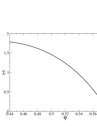
Figure 1: The equilibrium complexity $\Sigma(\varphi)$ as a function of the packing fraction.

Finally, the expression for the replicated free energy in $d=3$ is

$$\begin{split}\beta\Phi(m,\varphi)&=\beta F_{eq}(\varphi)+\frac{3}{2}(1-m)\log[2\pi A^{*}(m)]\\ &+\frac{3}{2}(m-1)-\frac{3}{2}\log m\end{split}$$ (48)

Note that for Hard Spheres one has $\beta F_{eq}(\varphi)=-S(\varphi)$, $S$ being the total entropy of the liquid. We get then

$$\begin{split}\beta f^{*}(&m,\varphi)=\frac{\partial\beta\Phi}{\partial m}=-\frac{3}{2}\log[2\pi A^{*}(m)]\\ &+\frac{3}{2}(1-m)\frac{d\log A^{*}(m)}{dm}+\frac{3}{2}\frac{m-1}{m}\ ,\\ \Sigma(m&,\varphi)=m\beta f^{*}-\beta\Phi=S(\varphi)-\frac{3}{2}\log[2\pi A^{*}(m)]\\ &+\frac{3m}{2}(1-m)\frac{d\log A^{*}(m)}{dm}+\frac{3}{2}\log m\end{split}$$ (49)

For small enough density the system is in the liquid phase and $m$ is equal to 1 at the saddle point. For $m=1$ we have:

$$\begin{split}&\frac{\sqrt{A^{*}(1)}}{D}=\frac{1}{8Q_{0}\,\varphi\,Y(\varphi)}\\ &S_{vib}(\varphi)\equiv-\beta f^{*}(1,\varphi)=\frac{3}{2}\log[2\pi A^{*}(1)]\\ &\Sigma(\varphi)=S(\varphi)-S_{vib}(\varphi)\end{split}$$ (50)

This allows for a computation of $\Sigma(\varphi)$ once $S(\varphi)$ and $Y(\varphi)$ are known. Note that $1+4\varphi Y(\varphi)=\beta P/\rho=-\varphi\frac{\partial S}{\partial\varphi}$, so a model for $S(\varphi)$ (or $Y(\varphi)$) is enough to determine all the quantities of interest.

V Results from the HNC free energy

We computed numerically $S(\varphi)$ and $Y(\varphi)$ solving the classical HNC equation for the Hard Sphere liquid up to $\varphi=0.65$. This allows to compute $\beta\Phi(\varphi,m)$ and gives access to all the thermodynamic quantities using Eq.s (49) and (50). In this section we discuss the results of this computation. We will set the sphere diameter $D=1$ in the following.

V.1 Equilibrium complexity

The equilibrium complexity $\Sigma(\varphi)$ is given by Eq. (50). It is reported in Fig. 1. We get a complexity $\Sigma\sim 1$ as found in previous calculations in Lennard-Jones systems MP99 ; CMPV99 ; MP99b ; MP00 , as well as in the numerical simulations CMPV99 ; SKT99 . The complexity vanishes at $\varphi_{K}=0.582$, that is the ideal glass transition density –or Kauzmann density– predicted by the HNC equations.

V.2 Phase diagram in the $(\varphi,m)$ plane

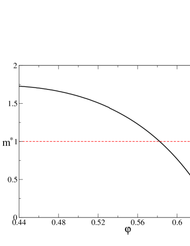
Figure 2: Phase diagram of the molecular liquid. For $m<m^{*}$ (full line) the system is in the liquid phase, for $m>m^{*}$ it is in the glass phase.

We now compute the thermodynamic properties of the glassy phase for $\varphi>\varphi_{K}$. As discussed above, it exists a value of $m$, $m^{*}(\varphi)$, such that for $m<m^{*}(\varphi)$ the system is in the liquid phase. It is the solution of $\Sigma(m,\varphi)=0$, where $\Sigma(m,\varphi)$ is given by Eq. (49). In Fig. 2 we report $m^{*}$ as a function of $\varphi$. Clearly, $m^{*}=1$ at $\varphi=\varphi_{K}$ and $m^{*}<1$ for $\varphi>\varphi_{K}$. $m^{*}$ vanishes linearly at $\varphi_{c}=0.640$. As we will see in the following, above this value of $\varphi$ the glassy state does not exist anymore.

V.3 Thermodynamic properties of the glass

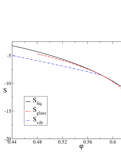
Figure 3: Entropy of the liquid (full line) and of the glass (dashed line). The two curves intersect at $\varphi_{K}=0.582$ where they are tangent and consequently the pressure is continuous at the glass transition. The entropy of the glass goes to $-\infty$ at $\varphi=\varphi_{c}=0.640$, so the glassy phase does not exist above $\varphi_{c}$. The dot–dashed line is the entropy of the equilibrium states of the liquid, $S_{vib}(\varphi)=S(\varphi)-\Sigma(\varphi)$.

The knowledge of the function $m^{*}(\varphi)$ allows to compute the entropy of the glass. Indeed, the free energy does not depend on $m$ in the whole glassy phase, and it is continuous along the line $m=m^{*}(\varphi)$, so we can compute the entropy of the glass simply as

$$S_{glass}(\varphi)=-\beta F_{glass}(\varphi)=-\frac{\beta\Phi(m^{*}(\varphi),\varphi)}{m^{*}(\varphi)}$$ (51)

This relation is true for $m^{*}<1$. Below $\varphi_{K}$ one has $m^{*}>1$ and the liquid phase is the stable one. Eq. (51) for $m^{*}>1$ gives the entropy of the lowest states in the free energy landscape (see below) and can be regarded as the analytic continuation of the glass entropy below $\varphi_{K}$. The reader should notice that the glass phase for $m^{*}>1$ does not have a simple physical meaning and the interesting part of the curves for the glass is in the region $\varphi>\varphi_{K}$.

In Fig. 3 we report the entropies of the liquid and the glass as functions of the packing fraction. The glass phase becomes stable above $\varphi_{K}=0.582$; note that the entropy of the glass is smaller than the entropy of the liquid, i.e. its free energy is bigger than the free energy of the liquid. The same happens also in Lennard-Jones systems and in mean-field spin glass systems. However the physical relevant parts of the curves are the liquid one for $\varphi<\varphi_{K}$ and the glassy one for $\varphi>\varphi_{K}$.

The reduced pressure,

$$\frac{\beta P}{\rho}=-\varphi\frac{\partial S}{\partial\varphi}\ ,$$ (52)

is reported in Fig. 4.

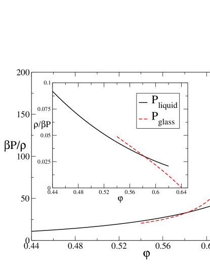
Figure 4: Reduced pressure $\beta P/\rho$ of the liquid and the glass as functions of the packing fraction. The pressure is continuous at $\varphi_{K}$. In the inset, the inverse reduced pressure is plotted; in the glass phase it is proportional to $\varphi_{c}-\varphi$.

It is continuous at $\varphi_{K}$ and the glass transition is a second order transition from the thermodynamical point of view. Note that the pressure in the glass phase is well described by a power law and it has a simple pole at $\varphi_{c}$:

$$\frac{\beta P_{glass}}{\rho}\propto\frac{1}{\varphi_{c}-\varphi}\ ,$$ (53)

as one can see from the inset of Fig. 4 where the inverse reduced pressure is plotted as a function of $\varphi$.

For $\varphi\rightarrow\varphi_{c}$ the pressure of the glass diverges and its compressibility $\chi=\frac{1}{\varphi}\frac{\partial\varphi}{\partial P}$ vanishes and consequently $\varphi_{c}$ is the maximum density allowed for a disordered state, i.e. it can be identified as the random close packing density. The value $\varphi_{c}=0.640$ is in very good agreement with the values reported in the literature. Note that the compressibility jumps downward on increasing $\varphi$ across $\varphi_{K}$, i.e. the compressibility of the glass is smaller than the compressibility of the liquid.

V.4 Cage radius

The cage radius is given as a function of $m$ in Eq. (47). In Fig. 5 we report the cage radius in the liquid phase, $\sqrt{A^{*}(1)}$, see Eq. (50), and the cage radius in the glass phase, defined as $\sqrt{A^{*}(m^{*})}$. As $Q_{m}\sim\sqrt{\pi/4m}$ for $m\sim 0$, the cage radius vanishes as $\sqrt{m^{*}}$ for $m^{*}\sim 0$, i.e. it is proportional to $\sqrt{\varphi_{c}-\varphi}$. The vanishing of the cage radius for $\varphi\rightarrow\varphi_{c}$ means that at $\varphi_{c}$ each sphere is in contact with its neighbors, that is consistent with our interpretation of $\varphi_{c}$ as the random close packing density.

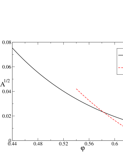
Figure 5: Cage radius $\sqrt{A}$ (in units of $D$) in the liquid and in the glass phase as function of $\varphi$.

V.5 Complexity of the metastable states

From the parametric plot of $\beta f^{*}(m,\varphi)$ and $\Sigma(m,\varphi)$ given in Eq. (49) by varying $m$, one can reconstruct the function $\Sigma(\beta f)$ for each value of the packing fraction. This function is reported in Fig. 6 for some values of $\varphi$ below and above $\varphi_{K}$. The function $\Sigma(\beta f)$ vanishes at a certain value $\beta f_{min}$, that is given by Eq. (51). The saddle-point equation that determines the free energy of the equilibrium states is, from Eq. (1),

$$\frac{d\Sigma(\beta f)}{d\beta f}=1\ .$$ (54)

From Fig. 6 we see that this equation has a solution $f^{*}>f_{min}$ for $\varphi<\varphi_{K}=0.582$. Above $\varphi_{K}$ Eq. (54) does not have a solution so the saddle point is simply $f^{*}=f_{min}$ and the systems goes in the glass state. In this sense, the free energy $f_{min}$ of the lowest states below $\varphi_{K}$ can be regarded as the analytic continuation of the free energy of the glass, see Fig. 3. The curves $\Sigma(\beta f)$ in Fig. 6 have been truncated arbitrarily at high $\beta f$. We have not done consistency checks to investigate where the higher free energy states become unstable (i.e. , to compute $f_{max}$).

VI Correlation functions

We will now turn to the study of the pair distribution function $\tilde{g}(r)$ in the glass state. In principle a full computation would require the evaluation of the corrections proportional to $\sqrt{A}$ in the correlation functions of a molecule. However we neglect these terms, that we believe are small, and we consider again our simple ansatz (11), (14) for the correlation function of the molecules, in which the information on the shape of the molecule is only encoded in the function $\rho(x)$; these corrections should be physically more relevant and interesting.

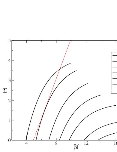
Figure 6: Complexity of the metastable states as a function of their free energy $\beta f$ for different values of $\varphi$. From left to right, $\varphi=0.45,0.5,0.55,0.58,0.6,0.62,0.63$. The curves are truncated arbitrarily at high $\beta f$. The dashed line has slope $1$.

As we will see in the following, the correlation function of the spheres in the glass is very similar to the one in the liquid but develops an additional strong peak (that becomes a $\delta$-function at $\varphi_{c}$) around $r=D$. The integral of the latter peak is related to the average coordination number of the random close packings.

VI.1 Expression of $\tilde{g}(r)$ in the glass phase

We assumed the following form for the pair distribution function of the molecular liquid, see Eq.s (11) and (14):

$$\begin{split}&\rho_{2}(x,y)=\rho(x)g(x,y)\rho(y)=\\ &\widehat{\rho}^{2}\int dXdY\prod_{a=1}^{m}\rho(x_{a}-X)g(|x_{a}-y_{a}|)\rho(y_{a}-Y)\ .\end{split}$$ (55)

The pair correlation $\tilde{g}(r)$ of a single replica is obtained integrating over the coordinates of all the replicas but one:

$$\tilde{g}(|x_{1}-y_{1}|)=\widehat{\rho}^{-2}\int d{\underline{x}}_{2}\cdots d{\underline{x}}_{m}d{\underline{y}}_{2}\cdots d{\underline{y}}_{m}\rho_{2}(x,y)\ .$$ (56)

Using Eq. (55) we get, with some simple changes of variable:

$$\tilde{g}(r)=g(r)\int d{\underline{u}}d{\underline{v}}\rho({\underline{u}})\rho({\underline{v}})F_{0}(|{\underline{r}}+{\underline{u}}-{\underline{v}}|)^{m-1}\ ,$$ (57)

where $F_{0}(r)$ is defined in Eq. (16). The HNC free energy is optimized by $g(r)=G(r)^{1/m}$, where $G(r)$ is the HNC pair correlation. Thus we get the following expression for the pair correlation of a single replica:

$$\begin{split}&\tilde{g}(r)=G(r)^{\frac{1}{m}}\int d{\underline{u}}\frac{e^{-\frac{u^{2}}{4A}}}{(\sqrt{4\pi A})^{d}}F_{0}(|{\underline{r}}+{\underline{u}}|)^{m-1}\ ,\\ &F_{0}(r)=\int d{\underline{u}}\frac{e^{-\frac{u^{2}}{4A}}}{(\sqrt{4\pi A})^{d}}G(|{\underline{r}}+{\underline{u}}|)^{\frac{1}{m}}\ .\end{split}$$ (58)

For $m=1$, i.e. in the liquid phase, this function is trivially equal to $G(r)$. This is not the case in the glass phase where $m<1$.

VI.2 Small cage expansion of the correlation function

We will now expand Eq. (58) for small $A$. Note first that, if $r\neq D$, the function $g(r+u)$ can be expanded in powers of $u$, and the first correction to $\tilde{g}(r)$ is of order $A$. Then, as before, we will concentrate on what happens around $r=D$. As already discussed in section III, around $r=D$ we have, as in Eq. (34), $G(r)\sim Y\theta(r-D)$ and

$$F_{0}(r)\sim Y^{\frac{1}{m}}\Theta\left(\frac{r-D}{\sqrt{4A}}\right)\ ,$$ (59)

and Eq. (58) becomes

$$\tilde{g}(r)=Y\theta(r-D)\int d{\underline{u}}\frac{e^{-\frac{u^{2}}{4A}}}{(\sqrt{4\pi A})^{d}}\Theta\left(\frac{|{\underline{r}}+{\underline{u}}|-D}{\sqrt{4A}}\right)^{m-1}\ .$$ (60)

Applying the same argument we used in section III when studying the function $F_{0}(r)$ in dimension $d>1$, we can show that the integration over the coordinates $u_{\mu}$, $\mu\neq 1$, gives a contribution $O(A)$. Then we can rewrite, in any dimension $d$:

$$\begin{split}&\tilde{g}(r)\sim Y\theta(r-D)\int_{-\infty}^{\infty}du\frac{e^{-\frac{u^{2}}{4A}}}{\sqrt{4\pi A}}\Theta\left(\frac{r+u-D}{\sqrt{4A}}\right)^{m-1}\\ &=G(r)\left\{1+\int_{-\infty}^{\infty}\frac{dt}{\sqrt{\pi}}e^{-\left(\frac{r-D}{\sqrt{4A}}-t\right)^{2}}\left[\Theta(t)^{m-1}-1\right]\right\}\ ,\end{split}$$ (61)

defining the reduced variable $t=\frac{r+u-D}{\sqrt{4A}}$. The second term in the latter expression is a contribution localized around $r=D$.

VI.3 Number of contacts

To compute the average number of contacts, let us recall that the average number of particles in a shell $[r,r+dr]$, if there is a particle in the origin, is given by

$$dn(r)=\Omega_{d}r^{d-1}\widehat{\rho}\,\tilde{g}(r)dr\ .$$ (62)

Thus the number of contacts can be obtained from the correlation function $\tilde{g}(r)$. While the full computation of the correlation function is rather involved, here we limit ourselves to consider the second term in Eq. (61), which is proportional to a Gaussian with variance $O(\sqrt{A})$ that becomes a $\delta(|r|-D)$-function in the limit $A\rightarrow 0$.

The value of the number of spheres in contact with the sphere in the origin is given by

$$z=\Omega_{d}\widehat{\rho}\int_{D}^{D+O(\sqrt{A})}dr\,r^{d-1}\tilde{g}(r)\ .$$ (63)

The first term in Eq. (61) gives a contribution $O(\sqrt{A})$ that can be neglected. If we use $r\sim D$ and $G(r)\sim Y$ at the leading order in $\sqrt{A}$ we obtain, defining the variable $\epsilon=\frac{r-D}{\sqrt{4A}}$,

$$\begin{split}&z=\Omega_{d}D^{d-1}\widehat{\rho}Y\times\\ &\times\sqrt{4A}\int_{0}^{\infty}d\epsilon\int_{-\infty}^{\infty}\frac{dt}{\sqrt{\pi}}e^{-(\epsilon-t)^{2}}\left[\Theta(t)^{m-1}-1\right]\ .\end{split}$$ (64)

Recalling that

$$\frac{1}{\sqrt{\pi}}\int_{0}^{\infty}d\epsilon\,e^{-(\epsilon-t)^{2}}=\Theta(t)\ ,$$ (65)

we get, observing that $\int_{-\infty}^{\infty}dt\,\big{[}\Theta(t)-\theta(t)\big{]}=0$, and using Eq. (46),

$$\begin{split}z&=\Sigma_{d}(D)\widehat{\rho}Y\sqrt{4A}\int_{-\infty}^{\infty}dt\,\Theta(t)\left[\Theta(t)^{m-1}-1\right]\\ &=\Sigma_{d}(D)\widehat{\rho}Y\sqrt{4A}Q_{m}=2d(1-m)\ .\end{split}$$ (66)

This is the expression of the average number of contacts at the leading order in $\sqrt{A}$, to be computed at $m=m^{*}$ in the glass phase. At $\varphi=\varphi_{c}$, where $m^{*}=0$, each sphere has on average $2d$ contacts. This is exactly what is found in numerical simulations; the condition $z\geq 2d$ is required for the mechanical stability of the packings as can be understood by mean of a very simple argument Al98 .

Note that this result is independent on the particular expression we chose for $S(\varphi)$, $Y(\varphi)$ and $G(r)$, i.e. it might hold beyond the choice of HNC equations for the molecular liquid provided that the expression (46) for the cage radius is correct.

VII Discussion

We will now compare our results with related ones that appeared in the literature. The main obstacle for a quantitative comparison is that the HNC equations are known to yield a not very good description of the Hard Sphere liquid at high density Hansen ; typically one would obtain the right curves if one shifts the value of $\varphi$ of a quantity of order 0.03. Therefore, we should limit ourselves to a qualitative comparison of the results coming from the HNC equations with the results of numerical simulations. However, note that, although the expressions (47), (48) for the replicated free energy have been derived starting from the expression (6) for the HNC free energy, the final result depends only on the equilibrium entropy of the liquid $S(\varphi)$. It is interesting then, for the purpose of comparing our results with experiments and numerical simulations, to consider a more accurate model for $S(\varphi)$ in the liquid phase. We repeated the calculations of section V substituting the Carnahan–Starling (CS) entropy Hansen

$$\begin{split}&S_{CS}(\varphi)=-\log\left(\frac{6\varphi}{\pi e}\right)-\frac{4\varphi-3\varphi^{2}}{(1-\varphi)^{2}}\ ,\\ &Y_{CS}(\varphi)=\frac{1-\frac{1}{2}\varphi}{(1-\varphi)^{3}}\ .\end{split}$$ (67)

instead of the HNC entropy in Eq.s (48), (47). All the results of section V are qualitatively reproduced using the CS entropy, but the latter gives results in better agreement with the numerical data. However, this procedure is not completely consistent from a theoretical point of view: one should always keep in mind that our aim here is not to present a quantitative theory, but only to show that the replica approach yields a reasonable qualitative scenario for the glass transition in Hard Sphere systems.

VII.1 Complexity of the liquid and Kauzmann density

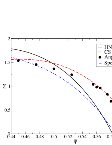
Figure 7: Equilibrium complexity $\Sigma(\varphi)$ as a function of the packing fraction. The full line is from the HNC equation of state (see Fig. 1), the dashed line is from the Carnahan–Starling equation of state. The black dots are numerical data of Angelani et al. Luca05 (the data shown here correspond to $\alpha_{0}^{(1)}$ in Ref. Luca05 ), the dot–dashed line is extrapolated from the numerical data reported by Speedy Sp98 .

In Fig. 7 we report the equilibrium complexity $\Sigma(\varphi)$ obtained substituting the HNC and the CS expression for $S(\varphi)$ and $Y(\varphi)$ in Eq. (50). The results are compared with recent numerical results of Angelani et al. Luca05 obtained on a $50:50$ binary mixture of spheres (to avoid crystallization) with diameter ratio equal to $1.2$: the vibrational entropy was estimated using the procedure described in CMPV99 ; AFST04 and the complexity was computed as $S(\varphi)-S_{vib}(\varphi)$. A quantitative comparison is difficult here because in the case of a mixture there can be corrections related to the mixing entropy, $S_{mix}\sim\log 2$. Nevertheless the data are in good agreement with our results. A detailed comparison would require the extension of our computation to binary mixtures following CMPV99 .

Another numerical estimate of $\Sigma(\varphi)$ was previously reported by Speedy Sp98 , who rationalized his numerical data assuming a Gaussian distribution of states and a particular form for the vibrational entropy inside a state. The free parameters were then fitted from the liquid equation of state. The curve obtained by Speedy also agrees with our results.

Both the HNC and the CS estimates of the Kauzmann density ($\varphi_{K}=0.582$ and $\varphi_{K}=0.617$ respectively) fall, as it should be, between the Mode–Coupling dynamical transition that is $\varphi_{MCT}\sim 0.56$ GS91 ; vMU93 , and the Random Close Packing density that is estimated in the range $\varphi=0.64\div 0.67$, see e.g. Be83 .

A computation of $\Sigma(\varphi)$ based on very similar ideas was presented in CFP98 , where a very similar estimate of $\varphi_{K}\sim 0.62$ was obtained. However in CFP98 the complexity was found to be $\Sigma\sim 0.01$, i.e. two orders of magnitude smaller than the one obtained from the numerical simulations. This negative result is probably due to some technical problem in the assumptions of CFP98 .

VII.2 Equation of state of the glass

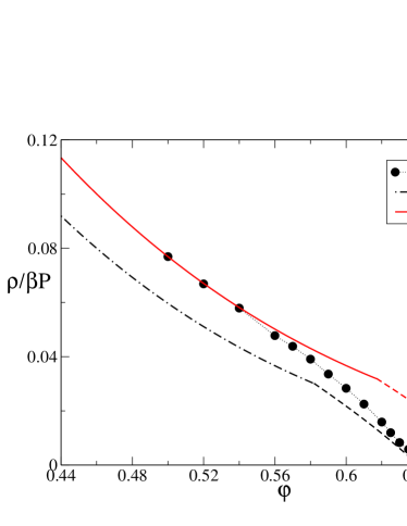
Figure 8: Inverse reduced pressure $\frac{\rho}{\beta P}$ of the Hard Sphere liquid as a function of $\varphi$. The black dots are from the simulation of Rintoul and Torquato RT96 . The full line is obtained from the CS equation of state while the dot–dashed line is from the HNC equation of state. The dashed parts of the two curves correspond to the (ideal) glass phase. Note that all the curves are quasi–linear functions of $\varphi$ in the glass phase.

In Fig. 8 we report as black dots the numerical data for the pressure of the Hard Sphere liquid at high $\varphi$ obtained by Rintoul and Torquato RT96 . The data were obtained extrapolating at long times the relaxation of the pressure as a function of time after an increase of density starting from an equilibrated configuration at lower density. We also report the curves of the pressure as a function of the density obtained from the HNC and CS equations, both in the liquid and in the glass state.

The agreement of the HNC curve with the data is not very good even in the liquid phase, due to the modest accuracy of the HNC equation of state. However, the qualitative behavior of our curve is in good agreement with the numerical data, and in particular the quasi–linear behavior of the inverse reduced pressure in the glass phase found in RT96 ; Sp98 , $\frac{\rho}{\beta P}\propto\varphi_{c}-\varphi$, is reproduced by the HNC curve. The HNC pressure of the glass diverges at $\varphi_{c}=0.640$ as discussed in section V; the latter is the HNC estimate of the random close packing density.

The CS curve describes well the pressure in the liquid phase Hansen . Comparing the curve with the data of Rintoul and Torquato, we see that the glass transition happens in the numerical simulation at a density $\varphi_{g}\sim 0.56$ smaller than the one predicted by the CS curve, $\varphi_{K}=0.617$ nota1 , and very close to the Mode–Coupling transition density, $\varphi_{MCT}\sim 0.56$. This is not surprising, since the relaxation time grows fast on approaching the ideal glass transition; at some point it becomes larger than the experimental time scale and the liquid falls out of equilibrium becoming a real glass. It is likely that the data of Ref. RT96 describe the pressure of a real nonequilibrium glass, while our computation gives the pressure of the ideal equilibrium glass, that cannot be reached experimentally in finite time.

VII.3 Random close packing

Both the HNC and CS equations predict the existence of a random close packing density $\varphi_{c}$ where the pressure and the value of the radial distribution function $\tilde{g}(r)$ in $r=D$ diverge. The HNC estimate is $\varphi_{c}=0.640$, in the range of the values ($\varphi_{c}=0.64\div 0.67$) reported in the literature. The CS estimate is $\varphi_{c}=0.683$ and it is also a value consistent with numerical simulations.

The reader should notice that the theoretical value for $\varphi_{c}$ is related to the ideal random close packing; however the states corresponding to this value of $\varphi_{c}$ can be reached by local algorithms, like most of the algorithms that were used in the literature, in a time that should diverge exponentially with the volume. Some caution should be taken in using the data obtained by numerical simulations. The question of which is the value of the density that can be obtained in large, but finite amount of time per particle is very interesting and more relevant from a practical point of view: however we plan to study it at a later time.

Note that the computation of the mean coordination number $z$ of section VI, that gives $z=6$ at $\varphi=\varphi_{c}$ in $d=3$, is independent of the particular form we choose for $S(\varphi)$, and thus is valid for both the HNC and CS equations of state. The value $z=6$ has been reported in many studies Be72 ; Ma74 ; Po79 ; Al98 ; SEGHL02 .

VIII Conclusions

We successfully applied the replica method of Mo95 ; MP99 to the study of the ideal glass transition of Hard Spheres, and in general of potentials such that the pair distribution function $g(r)$ shows discontinuities, starting from the replicated HNC free energy and expanding it at first order in the cage radius $\sqrt{A}$.

This result allowed us to compute from first principles the configurational entropy of the liquid as well as the thermodynamic properties of the glass up to the random close packing density. Our computation is based on the HNC equation of state, that is known to yield a poor quantitative description of the liquid state at high density. Nevertheless, we found that the qualitative scenario for the ideal glass transition that emerges from the replicated HNC free energy is very reasonable. In particular, we found a complexity $\Sigma\sim 1$, a Kauzmann density $\varphi_{K}=0.582$, and a random close packing density $\varphi_{c}=0.64$. All these results compare well with numerical simulations.

Using, on a phenomenological ground, the Carnahan–Starling equation of state instead of the HNC equation of state as input for our calculations, we could also compare our results with the high–density pressure data of Rintoul and Torquato showing that they are indeed compatible with the observation of a real glass transition.

Moreover, we found that the mean coordination number in the amorphous packed states is $z=2d$ irrespective of the equation of state we use for the liquid, in very good agreement with the result of numerical simulations and with theoretical arguments Be72 ; Ma74 ; SEGHL02 ; Al98 .

It is worth to note that our results do not prove the existence of a glass transition for the Hard Sphere liquid, as they derive from a particular approximation for the molecular liquid free energy (the HNC approximation), and, in general, other approximation such as the Percus–Yevick are possible Hansen .

- (1) M. D. Rintoul and S. Torquato, J. Chem. Phys. 105, 9258 (1996).
- (2) M. Robles, M. López de Haro, A. Santos and S. Bravo Yuste, J. Chem. Phys. 108, 1290 (1998).
- (3) R. J. Speedy, Mol. Phys. 95, 169 (1998).
- (4) M. Tarzia, A. De Candia, A. Fierro, M. Nicodemi and A. Coniglio, Europhys. Lett. 66, 531 (2004).
- (5) W. Götze and L. Sjögren, Phys. Rev. A 43, 5442 (1991).
- (6) W. van Megen and S. M. Underwood, Phys. Rev. Lett. 70, 2766 (1993).
- (7) F. H. Stillinger and T. A. Weber, Science 225, 978 (1984).
- (8) P. G. Debenedetti, Metastable liquids (Princeton University Press, NY, 1996).
- (9) B. Coluzzi, M. Mézard, G. Parisi and P. Verrocchio, J. Chem. Phys. 111, 9039 (1999).
- (10) F. Sciortino, W. Kob, P. Tartaglia, Phys. Rev. Lett. 83, 3214 (1999).
- (11) W. Kauzmann, Chem. Rev. 43, 219 (1948).
- (12) C. A. Angell, Science 267, 1924 (1995).
- (13) M. Mézard and G. Parisi, J. Chem. Phys. 111, 1076 (1999).
- (14) M. Cardenas, S. Franz and G. Parisi, J. Phys. A 31, L163 (1998); J. Chem. Phys. 110, 1726 (1999).
- (15) L. Angelani, G. Foffi and F. Sciortino, cond-mat/0506447.
- (16) J. G. Berryman, Phys. Rev. A 27, 1053 (1983).
- (17) G. D. Scott and D. M. Kilgour, Brit. J. Appl. Phys. (J. Phys. D) 2, 863 (1969).
- (18) J. L. Finney, Proc. R. Soc. London, Ser. A 319, 479 (1970).
- (19) C. H. Bennett, J. Appl. Phys. 43, 2727 (1972).
- (20) A. J. Matheson, J. Phys. C: Solid State Phys. 7, 2569 (1974).
- (21) M. J. Powell, Phys. Rev. B 20, 4194 (1979).
- (22) S. Alexander, Phys. Rep. 296, 65 (1998).
- (23) L. E. Silbert, D. E. Ertas, G. S. Grest, T. C. Halsey, and D. Levine, Phys. Rev. E 65, 031304 (2002).
- (24) M. Mézard, G. Parisi and M. A. Virasoro, Spin glass theory and beyond (World Scientific, Singapore, 1987).
- (25) R. Monasson, Phys. Rev. Lett. 75, 2847 (1995).
- (26) M. Mézard and G. Parisi, Phys. Rev. Lett. 82, 747 (1999).
- (27) M. Mézard and G. Parisi, J. Phys.: Condens. Matter 12, 6655 (2000).
- (28) J.-P. Hansen and I.R. McDonald, Theory of simple liquids (Academic Press, London, 1986).
- (29) L. Angelani, G. Foffi, F. Sciortino and P. Tartaglia, J. Phys.: Condens. Matter 17, L113 (2005).
- (30) Note that the authors of RT96 interpreted their data as showing no evidence for a glass transition, the pressure being a differentiable function of . However, as recognized in RLSB98 , their data are better described by a broken curve showing a glass transition around .