Bright solitons in coupled defocusing NLS equation supported by coupling: Application to Bose-Einstein Condensation

Abstract

We demonstrate the formation of bright solitons in coupled defocusing nonlinear Schrödinger (NLS) equation supported by attractive coupling. As an application we use a time-dependent dynamical mean-field model to study the formation of stable bright solitons in two-component repulsive Bose-Einstein condensates (BECs) supported by interspecies attraction in a quasi one-dimensional geometry. When all interactions are repulsive, there cannot be bright solitons. However, bright solitons can be formed in two-component repulsive BECs for a sufficiently attractive interspecies interaction, which induces an attractive effective interaction among bosons of same type.

Recently, there have been successful observation exp1 ; exp4 and associated theoretical yyy studies of two-component Bose-Einstein condensates (BEC). There have also been experimental observation sol of bright solitons in a BEC formed due to atomic attraction and related theoretical investigations solt . In fiber optics true one-dimensional solitons are formed in the nonlinear Schrödinger (NLS) equation 1 ; agra . The solitons of BEC sol are formed in a quasi-one-dimensional geometry achieved by employing a strong transverse trap. In either case, no solitons can be formed for repulsive interactions.

In this Letter we suggest the possibility of the formation of stable bright solitons in two-component BECs in the presence of repulsive interaction among like atoms and attractive interaction among atoms of different types. We find that a sufficiently strong interspecies attraction can induce an effective attraction among like atoms responsible for the formation of bright solitons in two-component BECs. We also consider similar two-component BECs in the presence of a periodic optical-lattice potential, which are now routinely used in experiments on BECs ol . We consider the formation of these solitons using a coupled time-dependent mean-field Gross-Pitaevskii (GP) equation 11 .

Because of two components such solitons of the coupled one-dimensional NLS equation are often termed vector solitons agra in nonlinear fiber optics, where two orthogonally-polarized pulses of different widths and peak powers in general propagate undistorted. The vector solitons considered so far in nonlinear optics were always created in focusing (attractive) medium. To the best of our knowledge the present study is the first to consider the possibility of creation of vector solitons in defocusing (repulsive) medium.

The experimental study of bright solitons in quasi-one-dimensional attractive systems is quite delicate due to the possibility of collapse in such systems, although a true one-dimensional system does not exhibit collapse 11 . The two-component repulsive BECs with interspecies attraction are better suited for studying solitons as such systems may not easily collapse ska and one can have a controlled study of solitons. Experimentally, this could be realized by forming a coupled repulsive BEC in a cigar-shaped geometry and then transforming the interspecies repulsion to attraction via a Feshbach resonance fs and eventually removing the axial trap so that the BEC components attain mobility in the axial direction like soliton under the action of radial trapping alone.

Bright solitons are really eigenfunctions of the one-dimensional NLS equation. However, the experimental realization of bright solitons in trapped attractive cigar-shaped BECs has been possible under strong transverse binding which, in the case of weak or no axial binding, simulates the ideal one-dimensional situation for the formation of bright solitons. The dimensionless NLS equation in the attractive or focusing case 1

$$iu_{t}+u_{xx}+|u|^{2}u=0,$$ (1)

sustains the following bright soliton 1 :

$$u(x,t) = \sqrt{2w}\hskip 3.0pt\mbox{sech}[\sqrt{w}(x-\delta+2vt)]$$ (2)

$$\times \exp[-iv(x-\delta)+i(w-vv)t+i\sigma],$$

with four parameters. The parameter $w$ represents the amplitude as well as pulse width, $v$ represents velocity, the parameters $\delta$ and $\sigma$ are phase constants. The bright soliton profile is easily recognized for $v=\delta=0$ when Eq. (1) leads to $|u(x,t)|=\sqrt{2w}\hskip 3.0pt\mbox{sech}(x\sqrt{w})$. In the case of the coupled focusing NLS equations:

$$iu_{t}+u_{xx}+(|u|^{2}+|v|^{2})u=0,$$ (3)

$$iv_{t}+v_{xx}+(|v|^{2}+|u|^{2})v=0,$$ (4)

one could have the following bright vector solitons agra ; mana : $u(x,t)=\cos(\theta)\sqrt{2w}\mbox{sech}(x\sqrt{w})\exp({it}),$ $v(x,t)=\sin(\theta)\sqrt{2w}\mbox{sech}(x\sqrt{w})\exp({it}),$ where $\theta$ is an arbitrary angle. Equations (3) and (4) are incoherently coupled as the coupling depends only on the intensities and is therefore phase insensitive. In this Letter we consider the vector solitons in Eqs. (3) and (4) with defocusing diagonal nonlinearities.

The time-dependent Bose-Einstein condensate wave function $\Psi({\bf r},t)$ at position ${\bf r}$ and time $t$ may be described by the following mean-field nonlinear GP equation 11

$$\biggr{[}-i\hbar\frac{\partial}{\partial t}-\frac{\hbar^{2}\nabla_{\bf r}^{2}}{2m}+V({\bf r})+gn\biggr{]}\Psi({\bf r},t)=0,$$ (5)

with normalization $\int d{\bf r}|\Psi({\bf r},t)|^{2}=1.$ Here $n\equiv|\Psi({\bf r},t)|^{2}$ is the boson probability density, $g=4\pi\hbar^{2}aN/m$, with $a$ the boson-boson scattering length, $m$ the mass and $N$ the number of bosonic atoms in the condensate. The trap potential with axial symmetry may be written as $V({\bf r})=\frac{1}{2}m\omega^{2}(\rho^{2}+\nu^{2}z^{2})$ where $\omega$ and $\nu\omega$ are the angular frequencies in the radial ($\rho$) and axial ($z$) directions with $\nu$ the anisotropy parameter, which will be taken to be 0 for axially free solitons in the following.

In the presence of two types of bosons each of mass $m,$ Eq. (5) gets changed to the following set of coupled equations ska :

$$\biggr{[}-i\hbar\frac{\partial}{\partial t}-\frac{\hbar^{2}\nabla_{\bf r}^{2}}{2m}+V({\bf r})+g_{11}n_{1}+g_{12}n_{2}\biggr{]}\Psi_{1}({\bf r},t)=0,$$

(6)

$$\biggr{[}-i\hbar\frac{\partial}{\partial t}-\frac{\hbar^{2}\nabla_{\bf r}^{2}}{2m}+V({\bf r})+g_{21}n_{1}+g_{22}n_{2}\biggr{]}\Psi_{2}({\bf r},t)=0.$$

Here $n_{i}\equiv|\Psi_{i}({\bf r},t)|^{2}$, $g_{ij}=4\pi\hbar^{2}a_{ij}N_{i}/m,\quad$ and $i,j=1,2$ represent the two types of bosons, and where $N_{1}$ is the number of boson 1 and $N_{2}$ that of boson 2, $a_{ij}$ is the scattering length for a boson of type $i$ and one of type $j$.

For the study of bright solitons we shall reduce Eqs. (Bright solitons in coupled defocusing NLS equation supported by coupling: Application to Bose-Einstein Condensation) and (Bright solitons in coupled defocusing NLS equation supported by coupling: Application to Bose-Einstein Condensation) to a minimal one-dimensional form in the cigar-shaped geometry with $\nu=0$. This is achieved by considering solutions of the type $\Psi_{i}({\bf r},t)=\phi_{i}(z,t)\psi^{(0)}(\rho)$ where

$$|\psi^{(0)}(\rho)|^{2} \equiv {\frac{m\omega}{\pi\hbar}}\exp\left(-\frac{m\omega\rho^{2}}{\hbar}\right).$$ (8)

The expression (8) corresponds to the ground state wave function in the absence of nonlinear interactions and satisfies

$$-\frac{\hbar^{2}}{2m}\nabla_{\rho}^{2}\psi^{(0)}(\rho)+\frac{1}{2}m\omega^{2}\rho^{2}\psi^{(0)}(\rho) = \hbar\omega\psi^{(0)}(\rho),$$ (9)

with normalization $2\pi\int_{0}^{\infty}|\psi^{(0)}(\rho)|^{2}\rho d\rho=1.$ Now the dynamics is carried by $\phi_{i}(z,t)$ and the radial dependence is frozen in the ground state $\psi^{(0)}(\rho)$.

Averaging over the radial mode, i.e., multiplying Eqs. (Bright solitons in coupled defocusing NLS equation supported by coupling: Application to Bose-Einstein Condensation) and (Bright solitons in coupled defocusing NLS equation supported by coupling: Application to Bose-Einstein Condensation) by $\psi^{(0)*}(\rho)$ and integrating over $\rho$, we obtain the following one-dimensional equations abdul :

$$\biggr{[}i\hbar\frac{\partial}{\partial t}+\frac{\hbar^{2}}{2m}\frac{\partial^{2}}{\partial z^{2}}-f_{11}|\phi_{1}|^{2}-f_{12}|\phi_{2}|^{2}\biggr{]}\phi_{{1}}(z,t)=0,$$ (10)

$$\biggr{[}i\hbar\frac{\partial}{\partial t}+\frac{\hbar^{2}}{2m}\frac{\partial^{2}}{\partial z^{2}}-f_{21}|\phi_{2}|^{2}-f_{22}|\phi_{2}|^{2}\biggr{]}\phi_{{2}}(z,t)=0,$$ (11)

where

$$f_{ij}=2\pi g_{ij}{\int_{0}^{\infty}|\psi^{(0)}|^{4}\rho d\rho}=g_{ij}{\frac{m\omega}{2\pi\hbar}}.$$ (12)

In Eqs. (10) and (11) the normalization is given by $\int_{-\infty}^{\infty}|\phi_{i}(z,t)|^{2}dz=1$.

For calculational purpose it is convenient to reduce the set (10) and (11) to dimensionless form by introducing convenient dimensionless variables. In Eqs. (10) and (11) we consider the dimensionless variables $\tau=t\omega/2$, $y=z/l$, ${\chi}_{i}=\sqrt{l}\phi_{i}$, with $l=\sqrt{\hbar/(\omega m)}$, so that we have the following coupled NLS equations

$$\biggr{[}i\frac{\partial}{\partial\tau}+\frac{d^{2}}{dy^{2}}-n_{11}\left|{{\chi}_{1}}\right|^{2}-n_{12}\left|{{\chi}_{2}}\right|^{2}\biggr{]}{\chi}_{{1}}({y},\tau)=0,$$ (13)

$$\biggr{[}i\frac{\partial}{\partial\tau}+\frac{d^{2}}{dy^{2}}-n_{21}\left|{{\chi}_{1}}\right|^{2}-n_{22}\left|{{\chi}_{2}}\right|^{2}\biggr{]}{\chi}_{{2}}(y,\tau)=0,$$ (14)

where $n_{ij}=4a_{ij}N_{i}/l,\quad i,j=1,2.$ In Eqs. (13) and (14), the normalization condition is given by $\int_{-\infty}^{\infty}|\chi_{i}(y,\tau)|^{2}dy=1.$

Equations (13) and (14) represent the one-dimensional limit of the three-dimensional equation. For solitons we finally have to take the nonlinearity coefficients $n_{ij}(i\neq j)$ to be negative corresponding to attraction. These equations have analytic solutions only under special conditions. First, when $n_{12}=n_{21}=0$, they become two uncoupled NLS equations which allow the following trivial soliton solutions for negative $n_{ii}$ 1 :

$$\chi_{i}(y,\tau)=\sqrt{(2w_{i}/|n_{ii}|)}\mbox{sech}(y\sqrt{w_{i}})\exp(i\tau),$$ (15)

$i=1,2.$ To satisfy the normalization condition one should have $w_{i}=n_{ii}^{2}/16$. In Eq. (15) and below the parameter $w$ is to be adjusted so as to satisfy the normalization condition. When all the nonlinear interactions are attractive (negative) and $n_{11}=n_{22}=-n$ and $n_{12}=n_{21}=-\alpha n$ one has the solutions 1

$$\chi_{i}(y,\tau)=\sqrt{[2w/(n\alpha+n)]}\mbox{sech}(y\sqrt{w})\exp(i\tau),$$ (16)

$i=1,2$, with $w=(n\alpha+n)^{2}/16$. Also, when $n_{ii}=0$, they have the following soliton solutions for negative nonlinearities

$$\chi_{i}(y,\tau)=\sqrt{(2w_{i}/|n_{ji}|)}\mbox{sech}(y\sqrt{w_{i}})\exp(i\tau),$$ (17)

$i\neq j,$ $i,j=1,2$ with $w_{i}=n_{ji}^{2}/16$. This case has the possibility of forming the soliton due to interspecies interaction as the intra-species interaction is zero.

It is also possible to have intra-species repulsion (positive or defocusing $n_{ii}$) and interspecies attraction (negative or focusing $n_{12}$ and $n_{21}$) in order to have the following soliton solutions of Eqs. (13) and (14) when $n_{11}=n_{22}=n$ and $n_{12}=n_{21}=-\alpha n,(\alpha>1):$

$$\chi_{i}(y,\tau)=\sqrt{[2w/(n\alpha-n)]}\mbox{sech}(y\sqrt{w})\exp(i\tau),$$ (18)

$i=1,2$ with $w=(n\alpha-n)^{2}/16$. In this case due to strong interspecies attraction solitons are formed despite of intra-species repulsion. In all these cases the functional dependence of the two analytic solutions $\chi_{i}(y,\tau)$ on $y$ are the same. However, there are interesting numerical solutions to Eqs. (13) and (14) where the functional dependence of $\chi_{i}(y,\tau),i=1,2,$ could be different, which we study next. Such vector solitons will have different widths and peak powers.

We solve the coupled mean-field-hydrodynamic equations (13) and (14) for bright solitons numerically using a time-iteration method based on the Crank-Nicholson discretization scheme elaborated in Ref. sk1 . We discretize the mean-field-hydrodynamic equation using time step $0.0005$ and space step $0.025$.

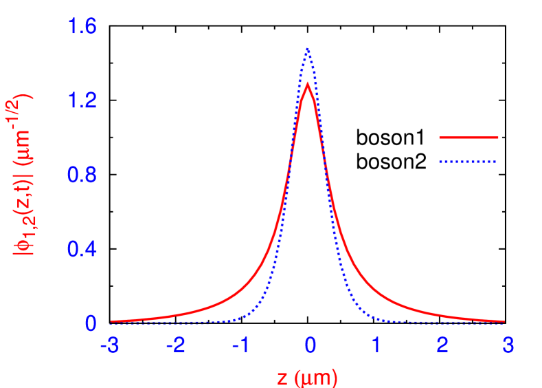
Figure 1: (a) The stationary functions $|\phi_{i}(z,t)|,i=1,2,$ for bosonic bright solitons vs. $z$ for $N_{1}=N_{2}=7500$, $a_{11}=1$ nm, $a_{12}=-1$ nm, and $a_{22}=0.1$ nm, harmonic oscillator length $l\approx 1$ $\mu$m and $\nu=0$. The nonlinearity parameters are $n_{11}=30$, $n_{12}=n_{21}=-30$, and $n_{22}=3$.

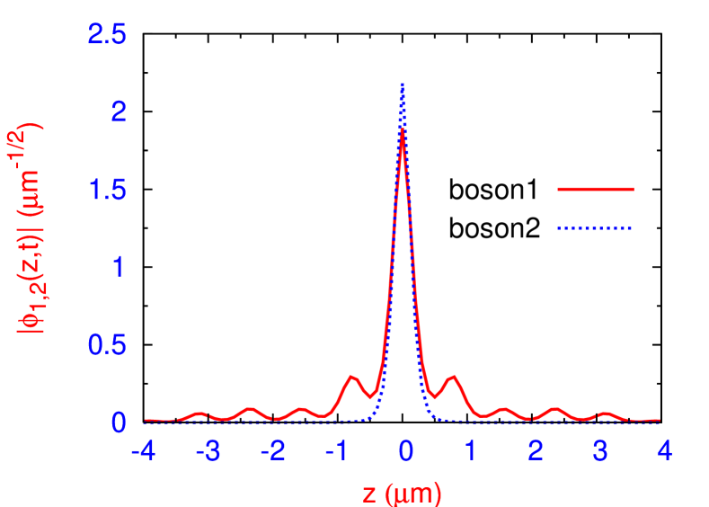
Figure 2: (a) The stationary functions $|\phi_{i}(z,t)|,i=1,2,$ for bosonic bright solitons vs. $z$ in the presence of the optical lattice potential $V(z)=100\sin^{2}(4z)$ in Eqs. (13) and (14). The nonlinearity parameters are $n_{11}=35$, $n_{12}=n_{21}=-30$, and $n_{22}=3$.

We performed the time evolution of the set of equations (13) and (14) introducing harmonic oscillator potentials $y^{2}$ in these equations and starting with the eigenfunction of the linear harmonic oscillator problem with the nonlinear terms set equal to zero: $\chi_{1}(y,\tau)=\chi_{2}(y,\tau)=\pi^{-1/4}\exp(-y^{2}/2)\exp(i\tau)$. During the course of time evolution the nonlinear terms are switched on very slowly and resultant solution iterated until convergence was obtained. Then the time evolution is continued and the harmonic oscillator potential terms ($y^{2}$) are slowly switched off and the resultant solution iterated 100 000 times for convergence. If converged solutions are obtained, they correspond to the required bright solutions. In the numerical investigation we take $\omega=2\pi\times 100$ Hz, and $m_{B}$ as the mass of ⁸⁷Rb. Consequently, the unit of length $l\approx 1$ $\mu$m and unit of time $2/\omega\approx 3$ ms.

First we solve Eqs. (13) and (14) with $N_{1}=N_{2}=7500$, $a_{11}=1$ nm, $a_{12}=-1$ nm and $a_{22}=0.1$ nm. With these parameters the nonlinearities in Eqs. (13) and (14) are $n_{11}=30$, $n_{12}=-30$, $n_{21}=-30$, and $n_{22}=3$.

The converged bright solitons are plotted in Fig. 1. In this case the function $\phi_{1}$ of the first component extends over a longer region in space compared to the function $\phi_{2}$ of the second component. It is possible to have solitons with different extensions in space by varying the parameters of the system. The scattering length can be manipulated in the bosonic systems near a Feshbach resonance fs by varying a background magnetic field. By varying the scattering length and the number of atoms we could arrive at different values of nonlinearity parameters from those in Fig. 1 and thus have different extensions of the condensates in space.

In the situation presented in Fig. 1, in Eq. (13) governing the dynamics of boson 1 the two nonlinearities are $n_{11}=30$ and $n_{12}=-30$, which may superficially indicate an effective nonlinearity of 0. However, the effective nonlinearity in this equation is $-n_{11}|\chi_{1}|^{2}-n_{12}|\chi_{2}|^{2}$. Due to a more strongly bound soliton of boson 2 this effective nonlinearity could become attractive and bind the soliton of type 1.

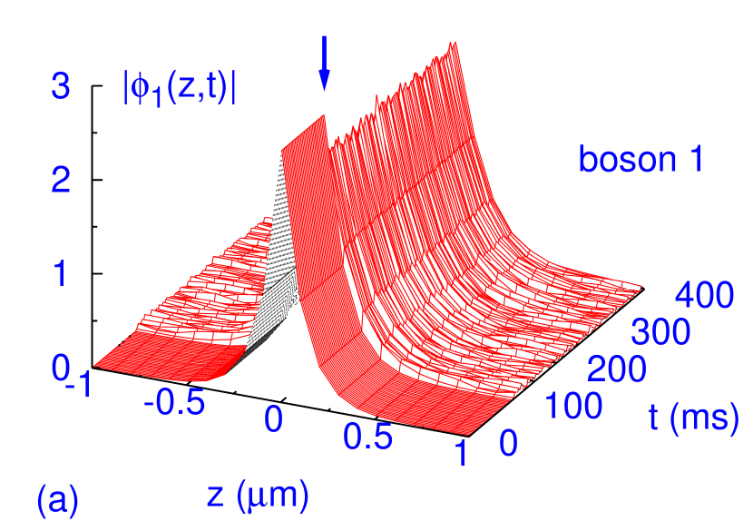
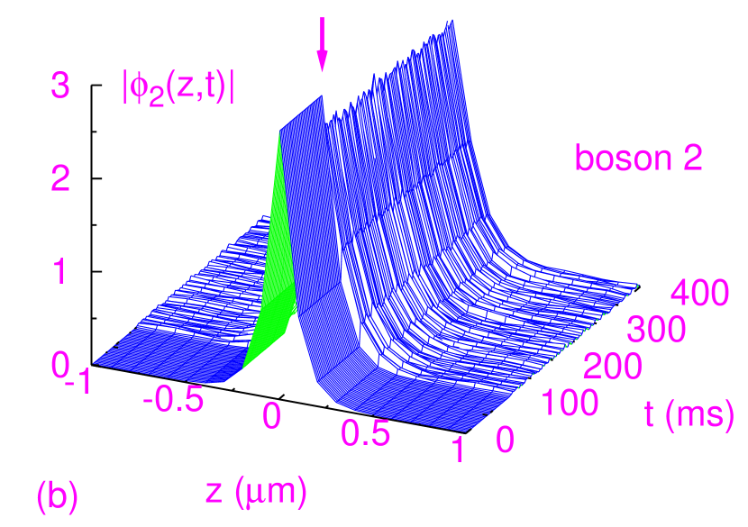
Figure 3: The function $|\phi_{i}(z,t)|$ for bosonic bright solitons vs. $z$ and $t$ for (a) boson 1 and (b) boson 2. At $t=0$ $N_{1}=N_{2}=7500$, $a_{11}=1$ nm, $a_{12}=-1.7$ nm, and $a_{22}=0.1$ nm, harmonic oscillator length $l\approx 1$ $\mu$m and $\nu=0$. The nonlinearity parameters at $t=0$ are $n_{11}=30$, $n_{12}=n_{21}=-51$, and $n_{22}=3$. At $t=100$ ms (marked by arrows) the two bright solitons are set into breathing oscillation by suddenly jumping the nonlinearities $n_{12}$ and $n_{21}$ to $n_{12}=n_{21}=-45$.

Next we consider a two-component soliton formed in the optical-lattice potential $V(z)=V_{0}\sin^{2}(4z)$ introduced in Eqs. (13) and (14). In our numerical calculation we take $V_{0}=100$, $n_{11}=35$, $n_{12}=n_{21}=-30$, and $n_{22}=3$. In this case in the wave function of boson 1 prominent wiggles are formed due to the optical-lattice potential. As the spacing of the optical-lattice sites are relatively large no wiggles are formed in the more localized wave function of boson 2. Equation (13) taken separately has nonlinearities $n_{11}=35$ and $n_{12}=-30$ corresponding to an apparent overall repulsion. However, the strongly bound soliton of boson 2 and the interspecies attraction as well as the periodic optical-lattice potential aid in the formation of the soliton of boson 1. In this connection it should be noted that the optical-lattice potential aids in binding the soliton in the presence of nonlinear interspecies attraction. The optical-lattice potential alone cannot bind a soliton in the absence of nonlinear attraction both in one- and two-component BECs.

Finally, we consider the stability of these solitons under a small perturbation. For this purpose we consider the solitons of Eqs. (13) and (14) formed for nonlinearities $n_{11}=-30$, $n_{12}=n_{21}=-51$, and $n_{22}=3$. The wave functions $\phi_{i}(z,t)$ of these solitons are shown in Figs. 3 (a) and (b) for $i=1,2$, respectively. To test their stability under small perturbation, after their formation, the nonlinearities $n_{12}$ and $n_{21}$ are suddenly changed to $-45$ at $t=100$ ms so that the solitons are set into motion. Such change in the nonlinearity can be achieved by a jump in the scattering length by manipulating a background magnetic field near a Feshbach resonance fs . The solitons are found to execute stable non-periodic breathing oscillations. The stability of these solitons after the perturbation is applied is demonstrated in Figs. 3.

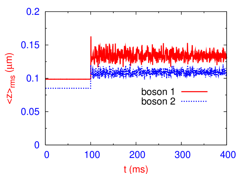
Figure 4: Root mean square size $\langle z\rangle_{\mbox{rms}}$ vs. time of the two solitons of Fig. 3 set into breathing oscillation by suddenly jumping the nonlinearities at $t=100$ ms.

To further illustrate the stability of the oscillation of the solitons of Figs. 3 we plot in Fig. 4 the root mean square (rms) size $\langle z\rangle_{rms}$ vs. time. Sustained oscillation for a very long time illustrates the stability of the solitons. From Fig. 4 we find that for $t<100$ ms the rms sizes of the two solitons are constant. However, after the application of the repulsive impulsive force at $t=100$ ms by reducing the attractive nonlinearity, the rms sizes suddenly jump to a larger value and execute stable oscillatory dynamics. This stable oscillation guaratees the stationary nature of the solitons under small perturbation.

The present investigation has consequences in generating bright vector solitons in directional couplers of nonlinear fiber optics agra . Vector solitons are solutions of coupled one-dimensional NLS equations with the property that the orthogonally polarized components propagate in a birefringent fiber without change in shape. In vector solitons an input pulse maintains not only its intensity profile but also its state of polarization even when it is not launched along one of the principal axes of the fiber. We have investigated the possibility that two orthogonally polarized pulses of different widths and different peak powers propagate undistorted in birefringent fibers. The present investigation suggests that it is possible to have bright vector solitons in the coupled NLS equation with diagonal defocusing (repulsive) nonlinearity and off-diagonal focusing (attractive) nonlinearity, which should be of interest in nonlinear fiber optics.

We use a coupled set of time-dependent mean-field GP equations for a two-component repulsive BEC to demonstrate the formation of bright solitons due to interspecies attraction. The interspecies attraction can neutralize the intra-species repulsion and induce an effective attraction in the mean-field GP equations responsible for the formation of bright solitons. An attractive interspecies interaction is necessary for the formation of the bright solitons as the diagonal nonlinearity $n_{ii}$ in the mean-field equations is taken to be repulsive (positive). In mean-field equations (13) and (14) $n_{ii}$s are positive (repulsive) and $n_{ij}$s are negative (attractive), so that the overall contribution of the nonlinear terms in these equations become attractive to support the bright solitons. We have also established the formation of these solitons in the presence of a periodic optical-lattice potential in an entirely different shape and trapping condition from a conventional soliton.

In view of the present study the appearance of bright solitons in multi-component repulsive BECs seems possible in quasi-one-dimensional geometry. Bright solitons have been created experimentally in attractive BECs in three dimensions in the presence of radial trapping only without any axial trapping sol . Also, there have been experimental studies of multicomponent BECs exp1 ; exp4 . Hence, bright solitons can be created and studied in the laboratory in the presence of radial trapping only in a two-component repulsive BEC supported by interspecies attraction and the prediction of the present study verified. We have also suggested the possibility of the formation of similar coupled solitons in fiber optics in one dimension.

Note added in proof: After the completion of this investigation we have known about another similar study sim .

- (1) D. S. Hall, M. R. Matthews, J. R. Ensher, C. E. Wieman, E. A. Cornell, Phys. Rev. Lett. 81 (1998) 1539; D. S. Hall, M. R. Matthews, C. E. Wieman, E. A. Cornell, Phys. Rev. Lett. 81 (1998) 1543; C. J. Myatt, E. A. Burt, R. W. Ghrist, E. A. Cornell, C. E. Wieman, Phys. Rev. Lett. 78 (1997) 586.
- (2) K. Xu, T. Mukaiyama, J. R. Abo-Shaeer, J. K. Chin, D. E. Miller, W. Ketterle, Phys. Rev. Lett. 91 (2003) 210402; E. Hodby, S. T. Thompson, C. A. Regal, M. Greiner, A. C. Wilson, D. S. Jin, E. A. Cornell, C. E. Wieman, Phys. Rev. Lett. 94 (2005) 120402.
- (3) N. G. Berloff, Phys. Rev. Lett. 94 (2005) 120401 (2005); K. Kasamatsu, M. Tsubota, M. Ueda, Phys. Rev. Lett. 93 (2004) 250406 (2004); K. Kasamatsu, M. Tsubota, Phys. Rev. Lett. 93 (2004) 100402; E. A. Ostrovskaya, Yu. S. Kivshar, Phys. Rev. Lett. 92 (2004) 180405; A. Kuklov, N. Prokofév, B. Svistunov, Phys. Rev. Lett. 92 (2004) 030403.
- (4) K. E. Strecker, G. B. Partridge, A. G. Truscott, R. G. Hulet, Nature (London) 417 (2002) 150; L. Khaykovich, F. Schreck, G. Ferrari, T. Bourdel, J. Cubizolles, L. D. Carr, Y. Castin, C. Salomon, Science 296 (2002) 1290.
- (5) U. Al Khawaja, H. T. C. Stoof, R. G. Hulet, K. E. Strecker, G. B. Partridge, Phys. Rev. Lett. 89 (2002) 200404; S. K. Adhikari, New J. Phys. 5 (2003) 137; L. D. Carr, Y. Castin, Phys. Rev. A 66 (2003) 063602; V. Y. F. Leung, A. G. Truscott, K. G. H. Baldwin, Phys. Rev. A 66 (2002) 061602(R); V. M. Perez-Garcia, H. Michinel, H. Herrero, Phys. Rev. A 57 (1998) 3837.
- (6) Y. S. Kivshar, G. P. Agrawal, Optical Solitons - From Fibers to Photonic Crystals, Academic Press, San Diego, 2003, pp 278-302.
- (7) G. P. Agrawal, Nonlinear Fiber Optics, Second Edition, Academic Press, San Diego, 1995, pp 263-265.
- (8) F. S. Cataliotti, S. Burger, C. Fort, P. Maddaloni, F. Minardi, A. Trombettoni, A. Smerzi, M. Inguscio, Science 293 (2001) 843; M. Greiner, O. Mandel, T. Esslinger, T. W. Hansch, I. Bloch, Nature (London) 415 (2002) 39; O. Morsch, J. H. Müller, D. Ciampini, M. Cristiani, P. B. Blakie, C. J. Williams, P. S. Julienne, E. Arimondo, Phys. Rev. A 67 (2003) 031603(R).
- (9) F. Dalfovo, S. Giorgini, L. P. Pitaevskii, S. Stringari, Rev. Mod. Phys. 71 (1999) 463.
- (10) S. K. Adhikari, Phys. Rev. A 63 (2001) 043611; S. K. Adhikari, Phys. Lett. A 281 (2001) 265.
- (11) S. Inouye, M. R. Andrews, J. Stenger, H. J. Miesner, D. M. Stamper-Kurn, W. Ketterle, Nature (London) 392 (1998) 151; Ph. Courteille, R. S. Freeland, D. J. Heinzen, F. A. van Abeelen, B. J. Verhaar, Phys. Rev. Lett. 81 (1998) 69.
- (12) S. V. Manakov, Sov. Phys. JETP 38 (1974) 248.
- (13) F. K. Abdullaev, R. Galimzyanov, J. Phys. B 36 (2003) 1099.
- (14) S. K. Adhikari, P. Muruganandam, J. Phys. B 35 (2002) 2831; P. Muruganandam, S. K. Adhikari, J. Phys. B 36 (2003) 2501.
- (15) V. M. Perez-Garcia, J. Belmonte, cond-mat/0506405.